Fernando Luiz Pereira de Oliveira
NONPARAMETRIC INTENSITY BOUNDS FOR
THE DETECTION AND DELINEATION OF
SPATIAL CLUSTERS
Universidade Federal de Minas Gerais Instituto de Ciˆencias Exatas Departamento de Estat´ıstica
Programa de P´os-Gradua¸c˜ao em Estat´ıstica
NONPARAMETRIC INTENSITY BOUNDS FOR
THE DETECTION AND DELINEATION OF
SPATIAL CLUSTERS
Fernando Luiz Pereira de Oliveira
Tese de doutorado submetida `a Banca
Exami-nadora designada pelo Colegiado do Programa
de P´os-Gradua¸c˜ao em Estat´ıstica da Universidade
Federal de Minas Gerais, como requisito parcial
para obten¸c˜ao do t´ıtulo de Doutor em Estat´ıstica.
´
Area de Concentra¸c˜ao: Estat´ıstica e Probabilidade
Orientador: Luiz Henrique Duczmal
Co-orientador: Andr´e Luiz Fernandes Can¸cado
Dedicat´
oria
Dedico este trabalho a minha m˜ae Benedita, ao meu pai Jo˜ao, meu irm˜ao
Francisco, a minha Grazinha, minha cunhada Mariana e a Deus que me
acompanhou e acompanha em todos os momentos. Obrigado por me apoiarem
cada um com sua forma.
Agradecimentos
Agrade¸co a CAPES e FAPEMIG. Agrade¸co a todos que diretamente ou
in-diretamente vieram a contribuir para o desenvolvimento desta Tese. Em
especial agrade¸co ao Professor Orientador Amigo Luiz Henrique Duczmal,
Andr´e Luiz Fernandes Can¸cado e Anderson Ribeiro Duarte.
Abstract
There is considerable uncertainty in the disease rate estimation for
aggre-gated area maps, especially for small population areas. As a consequence the delineation of local clustering is subject to substantial variation. Consider
the most likely disease cluster produced by any given method, like SaTScan
Kulldorff [2006], for the detection and inference of spatial clusters in a map
divided into areas; if this cluster is found to be statistically significant, what could be said of the external areas adjacent to the cluster? Do we have enough
information to exclude them from a health program of prevention? Do all the areas inside the cluster have the same importance from a practitioner
perspective?
We propose a criterion to measure the plausibility of each area being part of a possible localized anomaly in the map. In this work we assess the
problem of finding error bounds for the delineation of spatial clusters in maps of areas with known populations and observed number of cases. A given map
with the vector of real data (the number of observed cases for each area) shall be considered as just one of the possible realizations of the random variable
likely cluster for each replicated map is detected and the corresponding m likelihood values obtained by means of the m replications are ranked. For each area, we determine the maximum likelihood value obtained among the most likely clusters containing that area. Thus, we construct the intensity
function associated to each area’s ranking of its respective likelihood value among them obtained values.
The method is tested in numerical simulations and applied for three differ-ent real data maps for sharply and diffusely delineated clusters. The intensity
bounds found by the method reflect the geographic dispersion of the detected clusters.
The proposed technique is able to detect irregularly shaped and multiple clusters, making use of simple tools like the circular scan. Intensity bounds
for the delineation of spatial clusters are obtained and indicate the plausibility of each area belonging to the real cluster. This tool employs simple
mathe-matical concepts and interpreting the intensity function is very intuitive in terms of the importance of each area in delineating the possible anomalies of
the map of rates. The Monte Carlo simulation requires an effort similar to the circular scan algorithm, and therefore it is quite fast. We hope that this
tool should be useful in public health decision making of which areas should be prioritized.
List of Figures
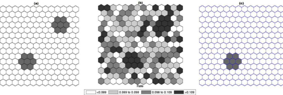
3.1 A single circularly shaped true artificial cluster with very high
relative risk (a), the random generated cases map of rates (b), and the cluster detected by the circular scan (c). . . 23
3.2 The intensity function (a) and the intensity bounds map (b) for the very high relative risk single circular cluster. . . 24
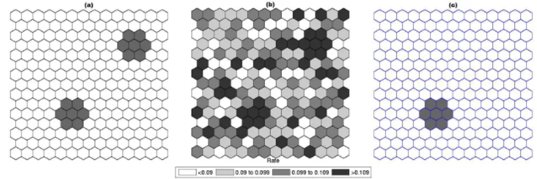
3.3 A single circularly shaped true artificial cluster with
moder-ately high relative risk (a), the random generated cases map of rates (b), and the cluster detected by the circular scan (c). . 24
3.4 The intensity function (a) and the intensity bounds map (b) for the moderately high relative risk single circular cluster. . . 25
3.5 The L-shaped true artificial cluster (a), the random generated
cases map of rates (b), and the cluster detected by the circular scan (c). . . 26
3.6 The intensity function (a) and the intensity bounds map for
the L-shaped artificial cluster. . . 27
3.7 A double circularly shaped true artificial cluster with very high
3.8 The intensity function (a) and the intensity bounds map (b) for the double circularly shaped cluster with very high relative
risk. . . 28
3.9 A double circularly shaped true artificial cluster with moder-ately high relative risk (a), the random generated cases map
of rates (b), and the cluster detected by the circular scan (c). . 29
3.10 The intensity function (a) and the intensity bounds map (b) for the moderately high relative risk double circular cluster. . 29
4.1 Homicide rates map (a) and population at risk map (b) in
Minas Gerais State, Brazil. . . 33
4.2 The intensity function for the homicides map. . . 33
4.3 The most likely cluster found by the circular scan (a) and intensity function map (b) for the homicides map. . . 34
4.4 The most likely cluster found by the circular scan (a) and
intensity function map (b) for the homicides map.(Zoom) . . . 34
4.5 The rates map (a) and population at risk map (b) for the Northeast U.S. breast cancer data. . . 35
4.6 The intensity function for the Northeast U.S. breast cancer data. 36
4.7 The three strongest clusters found by SaTScanKulldorff et al.
[1997] (a) and intensity function map (b) for the Northeast U.S. breast cancer data. . . 36
4.8 Chagas’ disease rates map (a) and population at risk map (b)
in Minas Gerais State, Brazil. . . 38
4.10 The most likely cluster found by the circular scan for the raw rates map (a), the raw rates intensity function map (b) and
Marshall’s smoothed rates intensity function map (c) for the Chagas’ disease map. . . 39
5.1 The most likely cluster of breast cancer among woman for the period 1988-1992, occurring sround New York, and
Philadel-phia, Pennsylvania, as well as four secondary clusters. . . 42
5.2 The intensity function map for the Northeast U.S. breast
can-cer data. . . 43
5.3 Three artificial clusters . . . 45
5.4 The three results for intensity function map (a) New York, (b) Boston and (c) Washington DC. . . 46
5.5 Most likely cluster found by genetic algorithm. . . 47
5.6 Cluster found by genetic algorith with maximum cluster size
was 5(a) and cluster found by genetic algorith with maximum cluster size was 10(b). . . 48
6.1 The intensity function for the raw rates map and the relative frequency map. . . 52
Contents
Abstract ix
List of Figures xi
Apresenta¸c˜ao 1
Motiva¸c˜ao . . . 1
Principais contribui¸c˜oes . . . 2
Organizac˜ao da Tese . . . 2
1 Introduction 5 2 Methods 9 2.1 Kulldorff’s Spatial Scan Statistic . . . 9
2.2 Single-Objective Genetic Algorithms . . . 11
2.3 Multi-objective Genetic Algorithms . . . 13
2.4 The intensity function . . . 15
2.5 Rate correction using empirical Bayesian estimator . . . 17
3 Results and Discussion 21 3.1 Numerical Simulations . . . 21
3.2 Single Circular Cluster . . . 22
3.4 Double Circular Cluster . . . 27
4 Real Data Case Studies 31 4.1 Homicide Clusters . . . 32
4.2 The Breast Cancer Clusters in Northeastern United States . . 35
4.3 Chagas’ Disease Clusters . . . 37
5 Irregulary shaped clusters 41 6 Relative Frequency Studies 51 7 Conclusions 53 Trabalhos Futuros 57 Produ¸c˜ao bibliogr´afica 59 References 61 8 Annexes 67 8.1 Annexe A - The weighted non-connectivity penalty . . . 67
8.1.1 The geometric penalty function . . . 67
8.1.2 The non-connectivity penalty function . . . 68
8.1.3 The weighted non-connectivity penalty . . . 69
8.1.4 Weighting the edges and nodes . . . 69
Apresenta¸
c˜
ao
Motiva¸
c˜
ao
Existe uma incerteza consider´avel na estimativa de taxas de doen¸cas para
mapas de ´area, especialmente para ´areas de popula¸c˜ao pequena. Como con-seq¨uˆencia, a delimita¸c˜ao do agrupamento local ´e sujeito a varia¸c˜oes
substan-ciais. Considere um cluster detectado por um determinado m´etodo, como SaTScan, para a detec¸c˜ao e inferˆencia de conglomerados espaciais em um
mapa dividido em ´areas. Se este cluster ´e considerado estatisticamente signi-ficativo, o que poderia ser dito das ´areas externas adjacentes ao cluster? N˜ao
temos informa¸c˜oes suficientes para exclui-las de um programa de preven¸c˜ao? Ser´a que todas as ´areas dentro do cluster tˆem a mesma importˆancia do ponto
de vista do usu´ario?
O problema de detec¸c˜ao de clusters espaciais encontra-se presente em diversas situa¸c˜oes, sendo importante determinar modelos satisfat´orios para
Principais contribui¸
c˜
oes
Nesta Tese desenvolvemos um novo conceito para a detec¸c˜ao e representa¸c˜ao
de clusters em mapas, descrevendo seus limites de erro. Tratamos um dos principais problemas em detec¸c˜ao de clusters, a medi¸c˜ao da incerteza da
defini¸c˜ao das ´areas que pertencem a um cluster detectado. A t´ecnica desen-volvida pode potencialmente ajudar em uma limita¸c˜ao existente ao utilizar
o scan circular, que ´e a n˜ao discrimina¸c˜ao entre os grupos que s˜ao mais ho-mogˆeneos daqueles que s˜ao mais irregulares ou em forma de anel. O m´etodo
proposto supera v´arias limita¸c˜oes em rela¸c˜ao `a estat´ıstica espacial scan: (i) conseguimos interpretar e delinear clusters diferentes do cluster prim´ario; (ii)
fornecemos uma interpreta¸c˜ao para a incerteza de ´areas que podem pertencer ao cluster. Al´em disso, esse m´etodo ´e computacionalmente muito r´apido.
Outra caracter´ıstica importante se refere `a interpreta¸c˜ao intuitiva desta nova metodologia, tornando o conceito f´acil de ser compreendido para os usu´arios.
Esperamos que a utiliza¸c˜ao desta nova metodologia seja utilizada por diversos profissionais de sa´ude p´ublica que fazem uso de busca de clusters geogr´aficos
para definir melhor suas prioridades.
Organizac˜
ao da Tese
Esta Tese est´a organizada da seguinte forma: no cap´ıtulo1apresenta-se uma
introdu¸c˜ao sobre trabalhos encontrados na literatura que abordam temas relacionados com a motiva¸c˜ao da metodologia desenvolvida, assim como a
descri¸c˜ao de t´ecnicas utilizadas para visualiza¸c˜ao e detec¸c˜ao de clusters ge-ogr´aficos. No cap´ıtulo2 descreve-se todas as metodologias que foram
utilizado na literatura. Neste cap´ıtulo apresentamos tamb´em o desenvolvi-mento da nova metodologia proposta nesta Tese, que chamamos de fun¸c˜ao
intensidade. No cap´ıtulo 3 apresentamos um estudo num´erico atrav´es de simula¸c˜oes em diversos tipos de mapas para testarmos a eficiˆencia da nossa
metodologia proposta. No cap´ıtulo4apresentamos a aplica¸c˜ao da metodolo-gia proposta em trˆes estudos de casos, utilizando como m´etodo de detec¸c˜ao de
cluster o scan circular. Nos cap´ıtulos 5e6utilizamos simula¸c˜oes para obser-var o comportamento da fun¸c˜ao intensidade com um m´etodo de detec¸c˜ao de
Chapter 1
Introduction
There are many methods for the detection and inference of geographic clus-tersCressie[1993],Elliott et al.[1995],Kulldorff[1999],Moore and Carpenter
[1999], Waller and Jacquez [2000], Lawson et al. [1999], Glaz et al. [2001],
Lawson [2001], Balakrishnan and V [2002],Buckeridge et al. [2005]. A large
number of methods rely on the Spatial Scan Statistic (Kulldorff [1997]), a development of the Naus spatial scan statistic (Naus [1965]). Based on this
statistic, several extensions were proposed, modifying the shape of the cir-cular window used in the circir-cular scan statistic (Kulldorff and Nagarwalla
[1995]) to include irregular shapes (Duczmal and Assun¸c˜ao [2004],Patil and Taillie [2004], Tango and Takahashi [2005], Kulldorff [2006], Duczmal et al.
[2006, 2007], Yiannakoulias et al.[2005]), see Duczmal et al. [2009] for a re-cent review. However, those methods generally do not discuss the possible
uncertainty in the delineation of the most likely cluster found. There exists nowadays a crescent demand of interactive software for the visualization of
spatial clusters (Hardisty and Conley [2008]).
their respective centroids, the procedure builds a grid of equidistant points between all combinations of two, three and four adjacent area centroids. For
each grid point the distances to the areas centroids are computed and sorted. These distances are used to define almost circular groupings of areas, with
their respective cumulative numbers of observed and expected cases. The relative risk and the likelihood ratio are then calculated for each circular
grouping. The likelihood ratio values are compared to the results of a Monte Carlo simulation under the null hypothesis that there are no clusters and
the cases are uniformly distributed in the population, such that the expected number of cases in each area is proportional to its population. Groupings with
likelihood ratios values exceeding 95% of those obtained from the simulation are stored and stratified into ten levels of relative risk. Within each risk
level, the grouping with largest likelihood ratio is then mapped. Circular groupings with lower likelihood ratio are also mapped if they did not overlap
any grouping previously mapped. The final result is a ten color shaded map of areas with statistically significant relative risks, providing a very effective
visualization tool to grasp these two concepts.
A visual tool was developed in Chen et al. [2008] to find circular clusters using SaTScan, repeating the search for a set of S different values for the maximum cluster size parameter. The reliability of an area ai is defined as the number of times this area is part of a significant circular cluster found
by SaTScan, divided by the number S. A typical value of S is 8, with maximum-sizes ranging from 5% to 49%, as given in the paper Chen et al.
[2008]. This approach allows the interactive visual identification the so-called “core clusters”, which are loosely defined as those clusters which appear more
although restricted to the circular shape delineation imposed by formalism of the circular scan.
The program SaTScan detects a spatial cluster in aggregated-area maps and compute its significance based on Monte Carlo simulations. This
ap-proach allows the characterization of a potential map anomaly, dividing the map into two areas, the cluster and the area outside it. In this work
pro-posed this thesis we are interested in pursuing further questions regarding the properties of individual areas inside and outside the detected cluster. We
would like to assess the relative importance of individual areas within the cluster. We would also like to verify if the areas outside the cluster and
ad-jacent to it could be indeed excluded from the suspected anomaly region in the map. These questions are important from a public health practitioner
perspective. How to access quantitatively the risk of those areas, given that the information we have (cases count) is also subject to variation in our
sta-tistical modeling? A few papers have tackled these questions recently. For example Rosychuk [2006] produces confidence intervals for the risk in every
area, which are compared to the risks inside the most likely cluster.
Geographic variability studies of disease rates are essential tools in eti-ology (Lawson [2009]). Maximum Likelihood Estimate Bayesian methods
have been proposed to obtain unbiased rates, especially for rare diseases occurring in small population areas (Efron and Morris [1973]), thus
provid-ing more precise results than the usual maximum likelihood estimators (see
Marshall[1991]). This approach includes information from adjacent areas to
estimate locally the risk, consequently reducing the quadratic mean error of the estimated rates. In Manton et al. [1981, 1987], Stone [1988] approaches
like-lihood with gamma prior distribution in disease mapping. The authors also presented a non-parametric estimation for the prior using a method which is
based on a spatial autoregressive procedure to model the prior distribution parameter devised by Laird [1978].
In this thesis, a different approach is proposed to delineate the “intensity bounds” associated to the most likely cluster, by running Monte Carlo
sim-ulations. The number of cases for each area is now considered as a random variable with mean equal to the observed rate, or to some smoothing function
which takes into account its first order neighborhood. We will introduce a novel approach to assess the relative importance of individual areas in the
composition of the clustering structure. The main purpose of our method is to find the error bounds for the delineation of spatial clusters in maps
divided into areas, through the definition of a criterion to measure the plau-sibility of each area being part of the cluster. As a by-product, our method
is capable of identifying irregularly shaped clusters and multiple local clus-tering. This method is computationally fast and relies on basic ideas about
the intrinsic variation of the observed number of cases for each area. This procedure allows the quantification of the uncertainty in the delineation of
Chapter 2
Methods
2.1
Kulldorff ’s Spatial Scan Statistic
Consider a map divided into k areas, with under-risk population N and C cases of an observable phenomenon. The analysis is conducted conditioned on the total number of cases so that C is considered a known constant. We define a zone as any setz of connected areas. Any circular window over the study area defines a zone z formed by areas whose centroids are inside the window.
Let Z be the set of all possible zones obtained by circular windows with varying radio and centered along each of the k areas centroids. The test proposed by Kulldorff [1997] is based on the maximization of the likelihood
ratio. The parameters set is (z;p;q) in which z denotes a zone in Z, p is the probability of an individual in z to be a case and q is the probability of an individual outside z to be a case. Such probabilities are constant for all individuals. Considering that there are no clusters within the map (null
like-lihood under the hypothesis that the zone z is a cluster (HA : p > q), and L0 the likelihood under the null hypothesis (H0 :p =q). Let n(z) and c(z) be, respectively, the population and cases inside z, and µ(z) = n(z)N C the expected number of cases insidez under the null hypothesis. For the Poisson model the likelihood function(Kulldorff [1997]) is:
L(z, p, q) = e
−pn(z)−q(N−n(z))
C! p
c(z)qC−c(z) m Y
j=1
n(j) (2.1)
The likelihood ratio, λ, can be written as
λ= SupHA{L(z)}
SupH0{L(z)} =
Supz∈Z,p>q{L(z, p, q)}
Supp=q{L(z, p, q)} =
L(ˆz)
L0 (2.2)
By definition, L0 = e
−C
C! C N
C Qm j=1
n(j).
Hence, likelihood ratio is expressed by
λ= Supz∈Z c(z) n(z) c(z) C−c(z) N−n(z)
C−c(z)
C N
C , if
c(z) n(z) >
C−c(z) N−n(z)
1 , otherwise
The distribution of (λ | C) must be obtained by a Monte Carlo simu-lation process (Kulldorff and Nagarwalla [1995]), since the distribution of
λ depends on the population distribution, what makes it almost impossible to be obtained analytically, and the usual assintotic aproximation via
Chi-square distribution, since the transformation −2logλ is not valid because regularity conditions are not satisfied.
A simplified form for the likelihood ratio is obtained considering
LR(z) = L(z) L0 =
I(z)c(z)O(z)C−c(z) , if I(z)>1
1 , otherwise
The most likely cluster is the zone ˆz that maximizes LR(z) (LR(ˆz) ≥
LR(z) ∀z ∈ Z). Since the logarithm is a strictly increasing function and LR(z) increases very quickly, it is more convenient to maximize LLR(z) = log{LR(z)}.
Alternatively we could detect a cluster simply considering the incidence of cases in each zone, that is, the ratio between the number of observed cases
and the population, or even the relative risk given by the number of observed cases divided by the expected number of cases. However, these measures do
not take into account that, a low populated zone will most likely present low significance, even if it presents high relative risk. The test based on theLLR (Kulldorff [1997]) bypass this problem since it also considers not only the relative number but also the absolute number of cases.
The statistical significance of the most likely cluster of observed cases is computed through a Monte Carlo simulation, according to Dwass [1957].
Under null hypothesis, simulated cases are distributed over the map and the scan statistic is computed for the most likely cluster. This procedure is
repeated many times, and the obtained distribution of the values is compared with the LLR of the most likely cluster of observed cases, producing an estimate of its p-value.
2.2
Single-Objective Genetic Algorithms
employed a strategy to “clean-up” the best configuration found in order to geometrically simplify the cluster. A genetic algorithm was used to find
clus-ters in point data sets, shaped as the inclus-tersections of circles with different sizes and centers (seeSahajpal et al. [2004]). In order to use the procedures
mentioned above , it is necessary to use some heuristic optimizer. Among the possible heuristics to be used in the detection spatial clusters problem,
genetic algorithm was implemented for the detection of clusters and inference in Duczmal et al. [2007] using the objective maximized the test Kulldorff’s
Scan statistic. The algorithm parts of an initial population of possible solu-tions in order to build a sequence of generasolu-tions. In the generasolu-tions, three
operators are used: crossover and mutation serve to increase the variability of the population of solutions and the selection operator chooses who will
be part of the next generation, directing the search and maintaining a fixed population size within a generation. The crossover operator creates new
in-dividuals (new zones), combining the features of two inin-dividuals (zones) were randomly chosen and named by parents A and B. Several new individuals are produced which are intermediate zones between the two extreme zones A and B. The mutation operator introduces random perturbations in the characteristics of an individual zone (adding or removing one random region) thus increasing the variability of the population. The selection operator
clas-sifies the zones according to the value of the objective function, in this case of the Spatial Scan statistic, choosing those which will be part of the next
generation. It is expected to find individuals (zones) with higher values for the objective function as the generations evolve. A geometric compactness
penalty function is employed to avoid excessive irregularity of the cluster ge-ometric shape. This algorithm is an order of magnitude faster and exhibits
as the Simulated Annealing Scan presented inDuczmal and Assun¸c˜ao[2004], and it is more flexible than the Elliptic Scan. It has about the same power of
detection as the Simulated Annealing Scan for mildly irregular clusters and it is superior for the very irregular ones.
2.3
Multi-objective Genetic Algorithms
Genetic algorithms are widely used for optimization problems in multi-objective, assessing the development of possible solutions, simultaneously evaluating
two or more objectives as in Fonseca and Fleming [1995], Takahashi et al.
[2003]. In Duczmal et al. [2007] it is suggested the use of Compactness
Ge-ometric penalty for a multi-objective Scan algorithm. In this proposal the penalty would be one of the objective functions, while the likelihood ratio
LLR(z) would be another objective function.
The pairs (LLRi, Ki), representing the logarithm of the Scan statistic value and Compactness (or other penalty function) computed for each
indi-vidual i (connected set of regions in the map) in the genetic population, are plotted in the Cartesian plane. The selection operator uses the concept of
dominance: a point is called dominated if it is worse than another point in at least one objective, while not being better than that point in any other
objective (seeChankong and Haimes[1983]). Thenon-dominated setconsists of all solutions which are not dominated by any other solution.
The construction of the initial population and the operators of crossover
and mutation are identical to those used in the single-objective genetic algo-rithm (seeDuczmal et al.[2007] for a detailed description of those operators).
the addition of newly produced offspring through the crossover operator. The next generation list, initially empty, stores the individuals that will survive
for the next generation. We compute the set of non-dominated solutions P0 of the current generation list, which is transferred to the initially empty next generation list; the same set P0 is also removed from the current gen-eration list. A new set P1 of the remaining individuals is computed, and the procedure is repeated until the new generation list has grown to con-tain M individuals, where M is the number of regions of the original map and corresponds to the population size that will be held constant along the generations. After a number of steps, say l, the set Pl will eventually not be totally added to the next generation list, because this would cause the list to contain more than M individuals. In such cases, the individuals of Pl are transferred randomly, one by one, until the next generation list contains exactly M individuals. This procedure is known as non-dominated sorting (see Deb et al.[2002]).
In the context of irregularly shaped clusters, the first of the competing objectives (regularity of shape) could not be considered appropriate if it was
the only objective of the search. If so, we would inevitably obtain a circularly shaped, but possibly meaningless, solution. Conversely, consider the
comple-mentary situation, when the maximization of the likelihood ratio, irrespec-tive of shape, is the only objecirrespec-tive: as we have seen in the introduction, this
would also produce solutions which are not useful from a geographic perspec-tive. The maximization of shape regularity only makes sense when coupled
with the maximization of likelihood ratio, as developed in the multi-objective methodology. Isolated, neither objective is sufficient to guide the search for
neighborhood connections with its adjacent regions compared to the number of component regions within the cluster due to the fact that its compactness
is high. Otherwise, an irregularly shaped cluster is probably “tree-like” in the sense that the number of connections with adjacent regions is small
com-pared to the number of component regions. In a situation where two clusters have the same LLR and one is more regularly shaped than the other, the former is preferred: the compactness of a cluster is generally related to the strength with which its component regions connect to each other. In this
regard, compactness is considered as a measure of stability of the cluster, as a solid geographic entity: we probably can remove a few regions from a
regularly shaped cluster without breaking it apart, but a similar operation may not be possible for a highly irregularly shaped cluster.
2.4
The intensity function
In this section we define a criterion to measure the plausibility of each area
being part of a possible localized anomaly in the map Oliveira et al. [2011]. Instead of finding the most likely cluster in the original map with the observed
number of cases for each area, we consider maps where the number of cases are replications of a vector of random variables, whose averages are defined
based on the observed number of cases of the original map. We formalize this procedure in the following.
The original map has ci observed cases in the area ai, i = 1, . . . , K. Now we construct a Monte Carlo replication distributing randomly theC = PK
si is the number of simulated cases in the area ai, i = 1, . . . , K, where PK
i=1si =C. The cluster finder algorithm (in our setting we use the circular scan or we use the elliptic scan) now finds the most likely clusterM LC1 with likelihood ratio value LLR1. The Monte Carlo procedure above is repeated m times, generating a set of m likelihood ratio values {LLR1, . . . , LLRm}
corresponding to the most likely clusters {M LC1, . . . , M LCm}. The likeli-hood ratio values are sorted in increasing order as {LLR(1), . . . , LLR(m)} for the corresponding most likely clusters found {M LC(1), . . . , M LC(m)}. We now define theintensityf unction
f :{1, . . . , m} −→R byf(j) =LLR(j),j = 1, . . . , m.
For each area ai, let:
q(ai) = 1
m arg 1≤j≤m,amaxi∈M LC(j)
f(j), i= 1, . . . , K
If the area ai does not belong to any of the sets M LC(1), . . . , M LC(m) then we set q(ai) = 0.
The value q(ai) represents the quantile of the highest likelihood ratio among the ranked values of the likelihood ratios of the most likely clusters
found in the m Monte Carlo replications, which take into account the vari-ability of the number of cases in each area. In this sense, the value q(ai) may be interpreted as the relative importance of the area ai as part of the anomaly of the map, where the value f(ai) represents the maximum likeli-hood ratio found for the most likely clusters which contain the areaai. This concept gives more information about the anomaly than the clear-cut
2.5
Rate correction using empirical Bayesian
estimator
We shall consider a variation of the procedure described in the previous
section. Instead of using the observed number of cases, this variant uses Marshall’s smoothed estimates of the number of cases based on the
informa-tion of first order neighborhood of each area. We then compute the intensity function in those two situations, employing the raw number of cases and
Marshall’s estimates.
Empirical Bayes methods were employed by Marshall [1991] and Yasui et al. [2000]. Studies involving disease rates to show the geographical
vari-ability are common in epidemiological approaches. For this kind of approach
it is important to assess the problem of obtaining unbiased estimates. Some Bayesian methods have been proposed in the literature for estimation of risks
in small areas. These methods are based on information from other areas that comprise the region of study. One consequence of using these
meth-ods is the decreasing of the total mean square error of the estimates Efron and Morris [1973]. That is, relative risks are estimated more accurately by
Bayesian methods than by using maximum likelihood estimation. Authors like Marshall [1991] andYasui et al. [2000] address this issue.
Efron and Morris [1973] were among the first to work with this approach
using empirical Bayes methods. Clayton and Kaldor[1987] proposed a proce-dure for empirical Bayes estimation using a Poisson likelihood and a gamma
priori distribution. One approach was suggested by Stone [1988] to adjust the significance levels in testing for geographical risks in excess, as well as in
method proposed by Laird [1978] who proposed a procedure to model the parameters of a priori distribution using a spatial autoregressive method.
Using Bayesian methods in the estimation of spatial phenomena have the extra advantage of allowing the incorporation of spatial similarities between
adjacent areas in risk estimates. Adding this information to the estimation of risk can lead to maps with more stable estimates and more precise
differ-entiation between what is a true high (or very low) risk and what is indeed a random fluctuation caused by small populations. Moreover, it is expected
that the estimates reproduce the spatial pattern of the real risks.
In this thesis we use the estimation procedure proposed byMarshall[1991] to obtain estimates of relative risks. We use local empirical Bayesian
estima-tors, because it is often reasonable to consider adjacent areas whose rates are similar because they are likely to be similar in other aspects. We use the first
order neighbors of the area for which we want to get the estimated rate. The methodology developed by Marshall proposed an empirical Bayesian
estima-tor for the risk of rare diseases, where one can approximate the distribution of the number of cases by the Poisson distribution with parameter estimated
by the method of moments. Consider a map divided intok areas indexed by i,i= 1,2, ..., k. Suppose that events are recorded for each area in a period of time. Letθi be the event rate in thei-th area and assume thatyi, the number of events accumulated in the i-th area during this period, is distributed as a Poisson random variable with mean E(yi|θi) = niθi, where ni is the pop-ulation at risk in the i-th area. The maximum likelihood estimator of θi is ti =yi/ni. This estimator has mean and variance conditioned onθi given by E(ti|θi) = θi and V(ti|θi) = θi/ni, respectively. In the Bayesian approach, θi has a prior distribution with mean mi =Eθi and variance Ai =Vθi.
Un-conditionally, ti has mean mi =Eti and variance Vti = Ai+
mi
Morris [1973] showed that, given mi and ai, the best linear Bayes estimator for θi is expressed by
ˆ
θi =witi+ (1−wi)mi
where wi = Ai
(Ai+mi/ni) is the a ratio between the a prior variance of θi and
the unconditional variance of ti. The global empirical Bayesian estimator proposed by Marshall [1991] assumes that the distribution of θi is the same for all areas and then replaces mi and Ai by m and A, respectively. Using the method of moments, Marshall showed that the estimates for m and A are given, respectively, by ˜m= PPyi
ni and ˜A =s
2− m˜ ¯
n, wheres
2 = PnPi(ti−m)˜
ni ,
¯
n = Pni
N and k is the number of areas of the map. As the overall proposal is spatially invariant, i.e., independent of the performed permutation, the
estimates do not change. It is necessary to change the expression of θi for the estimation of the a prior parameters set to be performed based on
in-formation from the neighboring areas of i. In this case, wi, m, s2 and n are replaced by Wi, Mi, s2i and ni, respectively, calculated only with data from the neighboring areas of i, and are defined as the local empirical Bayesian estimators.
Marshall’s smoothing procedure is advantageous when the number of cases is very small. It will be used for the Chagas’ disease map, which has a
Chapter 3
Results and Discussion
The methodology proposed in this thesis 2.4was tested in numerical
simula-tions and it was applied in three case studies.
3.1
Numerical Simulations
Three different types of “true” artificial clusters will be tested: a single cir-cular cluster (in two maps with different relative risks), a L-shaped irregular
cluster, and a double circular cluster (also in two maps with different rela-tive risks). In all situations, the map consists of a rectangular array of 203
hexagonal cells, each cell with population 1000. The centroids of the hexag-onal cells are not placed in a perfectly regular array; we introduced a slight
random displacement on bothxand yaxes, in order to avoid ties when mea-suring distances between any two centroids. Cases are randomly distributed
such that the cells inside the true cluster have higher probability of receiving cases than the areas outside it; the resulting maps with the randomly
inside and outside the artificial clusters. The clusters found by the circular scan are also shown. Finally, we display the resulting maps built through the
intensity function. Supposing a normal distribution of risks in the map, we consider very high relative risk clusters (the relative risk inside the cluster
is 5 standard deviations above the average global risk) and moderately high relative risk clusters (the relative risk inside the cluster is 3 standard
devia-tion above the average global risk). For a given map, the (greater than 1.0) risk is the same for all areas inside the cluster, and the risk is the same (1.0)
for all areas outside the cluster.
3.2
Single Circular Cluster
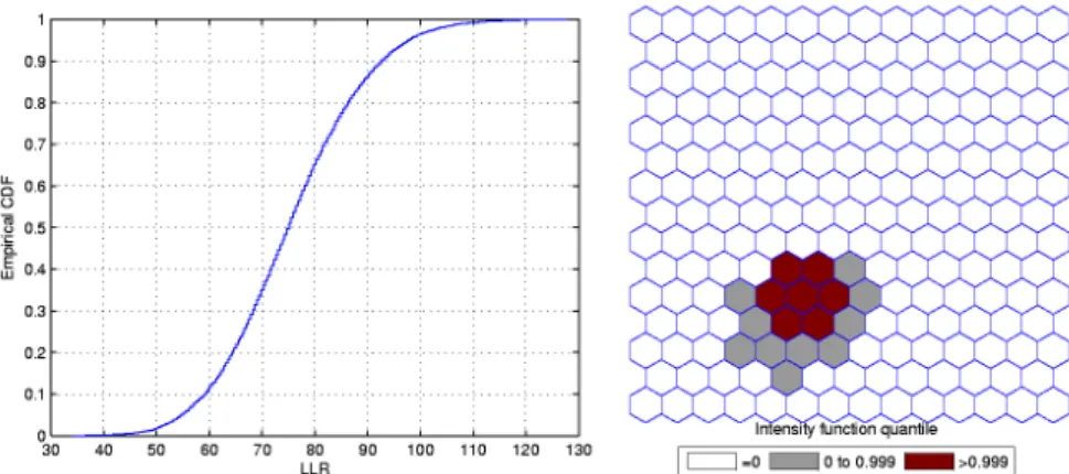
Figure 3.1 shows a circularly shaped true artificial cluster with very high
relative risk (a), the random generated cases map of rates (b), and the cluster detected by the circular scan (c). The intensity function is displayed in Figure
Figure 3.1: A single circularly shaped true artificial cluster with very high relative risk (a), the random generated cases map of rates (b), and the cluster
Figure 3.2: The intensity function (a) and the intensity bounds map (b) for
the very high relative risk single circular cluster.
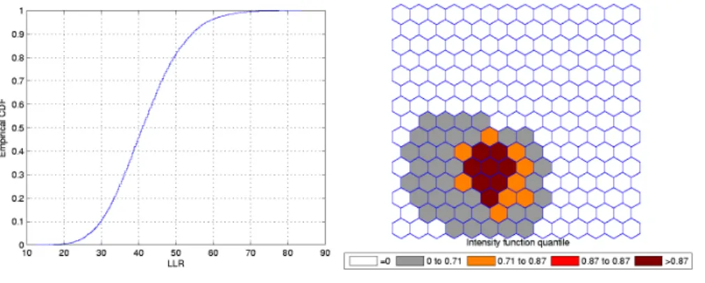
Figures 3.3 and 3.4 show the analogous results for another circularly
shaped true cluster, with moderately high relative risk, for comparison.
Figure 3.3: A single circularly shaped true artificial cluster with moderately high relative risk (a), the random generated cases map of rates (b), and the
Figure 3.4: The intensity function (a) and the intensity bounds map (b) for the moderately high relative risk single circular cluster.
The intensity bounds of the very high relative risk cluster are more sharply
defined than those corresponding to the moderately high relative risk cluster, as expected. Observe that in both instances the true clusters were clearly
detected, as represented by the darkest shade in Figures 3.2 and 3.4.
3.3
Irregularly Shaped Cluster
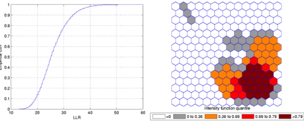
Figure 3.5shows a L-shaped true artificial cluster (a), the random generated
cases map of rates (b), and the cluster detected by the circular scan (c). The intensity function is displayed in Figure 3.6(a). The intensity bounds map
The circular scan detected a circular cluster centered in the angle formed by the two braces of the L-shaped cluster. However, the intensity bounds
roughly delineated the L-shape, with a more intense region located around the angle of the L-shaped cluster. Sometimes the realizations of the random
variable produced maps where circular clusters were found centered in the angle of the L-shaped cluster, but, very interestingly, also produced circular
clusters centered along the braces of the L-shaped cluster. As a result, the overall intensity map of Figure3.6indicates the form of the L-shaped cluster.
Figure 3.6: The intensity function (a) and the intensity bounds map for the L-shaped artificial cluster.
3.4
Double Circular Cluster
Figure 3.7 shows a double circularly shaped true artificial cluster with very high relative risk (a), the random generated cases map of rates (b), and the
cluster detected by the circular scan (c). The intensity function is displayed in Figure 3.8(a). Finally, the intensity bounds map obtained by our method
Figure 3.7: A double circularly shaped true artificial cluster with very high relative risk (a), the random generated cases map of rates (b), and the cluster
detected by the circular scan (c).
Figure 3.8: The intensity function (a) and the intensity bounds map (b) for
Figures3.9and3.10show the analogous results for another double circular true cluster, with moderately high relative risk, for comparison.
Figure 3.9: A double circularly shaped true artificial cluster with moderately
high relative risk (a), the random generated cases map of rates (b), and the cluster detected by the circular scan (c).
Figure 3.10: The intensity function (a) and the intensity bounds map (b) for the moderately high relative risk double circular cluster.
As displayed in Figures 3.7(b) and3.9(b), the local rates of the two com-ponents of the double cluster are not equal, and the circular scan detected
with a more intense region located around the highest risk circular compo-nent (Figures3.8(b) and3.10(b)). Sometimes the realizations of the random
variable produced maps where the highest risk circular component was found, but also produced circular clusters centered in the lower risk component. As a
Chapter 4
Real Data Case Studies
To illustrate the method proposed in this thesis, we present three real data case studies. In the first study, with homicide cases from Minas Gerais state,
Brazil, the most likely cluster is compact and very sharply delineated, with negligible geographic dispersion. The second study is a well-known
bench-mark of female breast cancer in the Northeast U.S. (Kulldorff [1997]), and the third case study displays Chagas’ disease cases in puerperal women, also
data from Minas Gerais state, Brazil. In those two last studies, the most likely clusters are not sharply delineated, presenting moderate geographic
dispersion. The breast cancer study has many cases, compared to the re-duced number of cases of the Chagas’ disease study, allowing us to compare
the performance of the map in two very different situations.
In the Chagas’ disease study we used both the raw and Marshall’s smoothed rates, due to the small number of cases. On the other hand, for the the other
two studies we have only presented raw rates results, because there are no advantages in employing smoothed rates when the raw rates are based in a
section. The choice of the quantile level representation by distinct shades of color varies in each map. We have chosen quantile levels in order to improve
the visualization of the intensity function in the maps. All blank areas were never part of any cluster in the Monte Carlo simulations, corresponding to
those areas ai for which q(ai) = 0. In the software, the user may choose arbitrary quantiles to represent the data. All the programming was made
using Matlab 7.10 and the code is available from the authors.
4.1
Homicide Clusters
Minas Gerais state is located in Brazil’s Southwest and consists of 853
mu-nicipalities, with 20,912 registered homicides from 2003 to 2007, and an esti-mated population of 19,150,344 in 2005. Data are available from the Brazilian
Ministry of Health (http:www.datasus.gov.br) and the Brazilian Institute of Geography and Statistics (http:www.ibge.gov.br).
The raw rates map is presented in Figure4.1(a) and the population at risk map in Figure4.1b. The Monte Carlo procedure described in the
Methodol-ogy section is performed for the raw rates, producing their respective intensity function. The intensity function for the raw rates map is displayed in
Fig-ure 4.2. Figure 4.3(a) shows the most likely cluster found by circular scan. Figure 4.3(b) show the map corresponding to the intensity function derived
Figure 4.1: Homicide rates map (a) and population at risk map (b) in Minas Gerais State, Brazil.
Figure 4.3: The most likely cluster found by the circular scan (a) and intensity
function map (b) for the homicides map.
Figure 4.4: The most likely cluster found by the circular scan (a) and intensity
function map (b) for the homicides map.(Zoom)
In the intensity function map, the non-blank areas attain almost the same level, meaning that the anomaly is very conspicuous. On the other hand, this
anomaly is compact and coincides with the most likely cluster found by the circular scan. Although there are other places in the map where the rates
4.2
The Breast Cancer Clusters in
Northeast-ern United States
The data set of mortality from breast cancer in the Northeastern U.S. consists
of age-adjusted 58,943 deaths for the period from 1988 to 1992, with the female population at risk of 29,535,210 in 1990. This map consists of 245
counties in 10 states and the District of Columbia. This dataset has been studied in detail using the circular spatial scan statistic (Kulldorff et al.
[1997]) and the elliptic spatial scan statistic (Kulldorff et al. [2006]). The raw rates map is presented in Figure 4.5(a) and the population at risk map
in Figure 4.5(b). The Monte Carlo procedure is performed producing its respective intensity function, displayed in Figure 4.6.
Figure 4.6: The intensity function for the Northeast U.S. breast cancer data.
Figure 4.7: The three strongest clusters found by SaTScan Kulldorff et al.
[1997] (a) and intensity function map (b) for the Northeast U.S. breast cancer
This case study presents a very different situation from the first example. The map derived from intensity function in Figure4.7(b) shows the presence
of various anomalies placed at different parts of the study area, indicat-ing their geographic dispersion. We clearly observe three distinct groups of
shaded areas in Figure4.7(b), consistently matching with the three strongest clusters found by SaTScan (Kulldorff et al. [1997]), shown in Figure 4.7(a).
The darkest shaded group is associated to the New York, NY-Philadelphia, PA primary cluster, with p-value 0.0001. The upper left group of four gray
areas coincides exactly with the Buffalo, NY secondary cluster, with p-value 0.122. Finally the gray area at the lower center of the map corresponds to
the Washington, DC secondary cluster, with p-value 0.147.
This example shows that the intensity function has the ability to delineate even the multiple and irregularly shaped potential clusters. We stress the fact
that, for each Monte Carlo replication, only the primary most likely cluster was used to build the map derived from the intensity function of Figure
4.7(b).
4.3
Chagas’ Disease Clusters
This subsection presents the data set of Chagas’ disease cases in puerperal women in Minas Gerais state, Brazil. The population at risk consists of
women that gave birth to babies in the period of July to September, 2006. The new-born babies were blood tested to detect the presence of the Chagas
disease antigen, with coverage above 96%. A positive test means that the mother is infected. These tests were conducted through the project
Minas Gerais Medical School (http:www.nupad.medicina.ufmg.br) in col-laboration with Minas Gerais State Health Secretary. The state is divided
into 853 municipalities with a total population at risk of 24,969 women. Af-ter a comprehensive screening to eliminate false positives a total number of
113 cases were obtained.
The raw rates map is presented in Figure 4.8(a) and the population at
risk map in Figure 4.8(b). The Monte Carlo procedure is performed for both the raw rates and Marshall’s smoothed rates maps, producing their
respective intensity functions. The intensity function for the raw rates map is displayed in Figure4.9(a). The intensity function for Marshall’s smoothed
rates is displayed in Figure 4.9(b). Figure 4.10(a) shows the most likely cluster found by circular scan. Figures 4.10(b) and 4.10(c) show the maps
corresponding to the intensity function derived from the raw rates map and the smoothed rates map, respectively.
Figure 4.8: Chagas’ disease rates map (a) and population at risk map (b) in
Figure 4.9: The intensity functions of the raw rates (a) and smoothed rates
(b) for the Chagas’ disease map.
Figure 4.10: The most likely cluster found by the circular scan for the raw rates map (a), the raw rates intensity function map (b) and Marshall’s
smoothed rates intensity function map (c) for the Chagas’ disease map.
The maps derived from the raw (Figure 4.10(b)) and smoothed (Figure
4.10(c)) intensity functions show the presence of a strong anomaly. For the map of Figure 4.10(b), the area formed by the highest intensity areas (dark
colored) coincides almost perfectly with the primary cluster found by the circular scan. However, the corresponding area of Figure 4.10(c) does not
dispersion of the anomaly, which spreads over the northern part of the state. This example shows that the error bounds of the existing cluster were easily
visualized by means of the intensity function. The application of Marshall’s smoothing procedure does not contribute to improve the delineation of the
Chapter 5
Irregulary shaped clusters
The circular spatial scan has several limitations, which were discussed in
the literature (Duczmal et al. [2006], Kulldorff et al. [2006]). In particular the circular window is not adequate to delineate irregularly shaped clusters
- either choosing a small proper subset of the cluster (underestimation) or choosing a large circle containing the cluster as a proper subset
(overestima-tion). One important consequence is the reduction of the power of detection. In order to overcome this limitation, many algorithms were proposed in the
last five years to detect irregularly shaped clusters, substituting the circu-larly shaped window. Usually, the only limitation in shape for those clusters
is a connectivity requirement. In this section, we will analyze the impact of irregularly shaped algorithms for the application of the intensity function
discusssed in the previous sections, compared to the use of the simple cir-cular scan, which was employed as the standard method. We will present
results only for the multi-objective genetic algorithm scan (Duczmal et al.
[2007,2008],Duarte et al. [2010]), adapted for the weighted non-connectivity
Figure 5.1: The most likely cluster of breast cancer among woman for the
Figure 5.2: The intensity function map for the Northeast U.S. breast cancer
The map derived from intensity function in Figure5.2shows the presence of various anomalies placed at different parts of the study area, indicating
their geographic focus. We observe several distinct groups of shaded areas in Figure5.2, consistently matching with the five strongest clusters found by
SaTScan (Kulldorff et al. [1997]), shown in Figure 5.1. The darkest shaded group spreads through a larger portion of the map (compared with the
cor-responding group found in chapter 4) and is associated to the New York, NY-Philadelphia, PA primary cluster, with p-value 0.0001. The same thing
happens with the upper left group of 13 gray areas, containing the Buffalo, NY secondary cluster of four areas, with p-value 0.122. Finally the gray area
at the lower center of the map corresponds to the Washington, DC secondary cluster, with p-value 0.147. The remaining two secondary clusters of Figure
5.1 have even higher p-values, and the corresponding groups in Figure 5.2
are less sharply defined. Other scattered groups also were formed through
the map.
This example shows that the intensity function has the ability to delineate
Figure 5.3: Three artificial clusters
We also present a set of simulations to illustrate the average behavior of the intensity function using the multiobjective genetic algorithm scan. We
generated 100 Monte Carlo replications for the construction of the intensity function, for each one of the three artificial clusters shown in Figure5.3. The
intensity function map was built and then we repeated the whole process 100 times, composing the average maps shown in Figure 5.4. We stress the fact
that this result is an average process, and we found a large variance in the delineation of the original clusters (Figure5.3), as expected. Even then, the
The same procedure was done for the Chagas’ disease map of Minas Gerais, representing a situation where the total number of cases is small.
5.5shows the most likely cluster of Chagas’ disease in Minas Gerais found by the multi-objective genetic algorithm. 5.6 displays the combined solutions of
the Pareto set, when the maximum cluster size was 5 (5.6(a)) and 10 (5.6(b)). The results show clusters considerably more sharply defined, compared to the
New England map’s clusters.
Figure 5.6: Cluster found by genetic algorith with maximum cluster size was 5(a) and cluster found by genetic algorith with maximum cluster size was
In conclusion, our examples using artificial and real data show that there is a palpable gain when using irregularly shaped methods. This gain is
trans-lated here as a greater sensitivity to detect boundaries of the clusters, and also the capacity to detect secondary clusters. However, the informational
gain is somewhat offset by the increased amount of detected noise, generated by the possibly excessive freedom of shape and/or size of the window used.
Smaller, more compact windows generate less noise, but also less sensitivity. The opposite is true for larger, less penalyzed (in terms of shape) windows,
which generate noiser maps with more clusters.
Our simulations seem to indicate that more complicated spatial
popula-tion distribupopula-tions, with several highly populated nuclei in different parts of the map, are better suited for the application of the intensity function with
the circular scan; otherwise, when the population is more evenly distributed, irregularly shaped algorithms may be more useful.
It is possible to find a balance between the informational gain, but cur-rently the most adequate parameters are not automatically chosen. A more
prudent strategy, in our setting, is to evaluate several simulations with differ-ent parameter settings. Further work is needed to assess the optimal choices
which could generate maps representing the adequate balance between noise and informational content. We presented results with the multi-objective
ge-netic algorithm scan, employing the weighted non-connectivity penalty func-tion. Other algorithms could also be used, but there is no reason to believe
that the basic features should be different, when using other types of algo-rithms. It seems that only the range of the window size, measured as the
maximum allowed population in the candidate clusters, is relevant to modify the balance of the algorithm’s sensitivity to detect secondary clusters and
Chapter 6
Relative Frequency Studies
One is tempted to ask if simpler criteria, aside from the intensity function
definition, should suffice for the delineation of the uncertainty bounds of spatial clusters. For instance a very simple frequentist approach could be used
instead: for each areaai, consider the numbermi of Monte Carlo replications when ai is included in a most likely cluster, divided by the total number of replicationsm. In Figure 6.1 we compare the intensity function map with the relative frequency map described above, for the New England breast cancer
map. It could be observed that the results are almost identical. On the other hand, Figure 6.2 makes a similar comparison for the Minas Gerais Chagas’
disease map. The results are considerably different; this happen because, for each area ai, the frequentist approach does not take into account the value of the highest LLR clusters which contain the area ai. The intensity function method, otherwise, does not produce underestimated LLR value
clusters. This difference is most notable when the number of cases in the map is small, and the relative variance is larger. When the total number of
Figure 6.1: The intensity function for the raw rates map and the relative
frequency map.
Chapter 7
Conclusions
Our methodology takes into account the variability in the observed number of
disease cases on area-aggregated maps to nonparametrically infer the uncer-tainty in the delineation of spatial clusters. A given real data map is regarded
as just one possible realization of an unknown random variable vector with expected number of cases. The real data vector of the number of observed
cases in each area is used to construct a new vector of expected values of random variables, either as a composition of neighboring areas in the map,
employing Marshall’s smoothing, or either considering the raw count of cases as the average of the random variables. This vector is now an estimate of
the unknown random variable vector with expected number of cases. Our methodology performs m Monte Carlo replications based on this estimated vector of averages. The most likely cluster of each replicated map is detected and the m corresponding likelihood values obtained in the replications are ranked. For each area we determine the maximum likelihood value among the most likely clusters containing that area. Thus, we obtain the intensity
importance of that area in the delineation of the possibly existing anomaly on the map, considering only the initially given information of the observed
number of cases. This procedure, based on empirical distribution, takes into account the intrinsic variability of the observed number of cases, which
gen-erally is not considered directly in the existing algorithms used to detect spatial clusters.
In our case studies we could see different situations with respect to the intrinsic variability of the existing spatial anomaly. When the most likely
cluster is quite prominent, as seen in the homicides map example, the in-tensity function is such that almost all areas associated with the most likely
clusters found in themreplications coincides with those areas composing the most likely cluster detected for the original observed cases. In this example
low geographic dispersion occurs. However, in the other two case studies, the opposite happens. The Chagas’ disease map presents an intrinsically wide
variability of data. Many areas near or adjacent to the most likely cluster have values of the intensity function close to the values corresponding to
ar-eas of the most likely cluster. In the case study of brar-east cancer, this intrinsic variability produces a map with clearly unrelated areas, but with rather close
probability ranking, indicating a situation of multiplicity of clusters, i. e., the most likely cluster is clearly poorly delineated. It is noteworthy that
the entire procedure was performed using the circular scan, and even then it identifies irregular and multiple clusters.
An analogy with our proposed method can be found in image analysis:
suppose we take several short digital exposures of a very low light level scene, e.g. some deep-sky field of galaxies. Each exposure generates an image
of the image. The expected rate of photons is constant during all the ex-posures, but the number of photons received by the same pixel varies from
one exposure to the other due to the stochastic nature of the process. Usu-ally, one simply adds the values for the same pixel through all the exposures,
to compose a single final image with higher sharpness (signal-to-noise). In-stead, we first submit each exposure image through a filter, which in our
case is the algorithm to detect the most likely cluster, and then compose all the corresponding clusters into a single “cluster image” by means of the
intensity function. If the “real” cluster is very contrasting with the back-ground noise, all exposures will produce very similar clusters, thus producing
a sharply defined final cluster image. Otherwise, when the real cluster is not very conspicuous, we should observe a large variation in individual clusters,
producing a poorly delineated cluster in the final image.
We presented two variants of the computation of the intensity function. The first employed the raw number of cases, and the second used Marshall’s
smoothed estimates of the number of cases based on the information of the first order neighborhood of each area. This was done because we were
espe-cially concerned with areas containing zero cases, which could generate biased Monte Carlo distributions of cases over the map. Marshall’s smoothed
es-timates of cases could potentially alleviate this problem providing non-zero averages employed in the multinomial random vector. However, we have
noted in all our examples that the application of Marshall’s smoothed es-timates produces less sharply defined intensity function maps, compared to
those obtained by the use of the raw cases data. On the other hand, we could not observe any artifacts due to the use of non-smoothed raw cases data in
areas within the circular window, thus naturally diminishing the effect of the zero cases areas in the composition of the cluster candidates. This suggests
that the utilization of raw cases data does not seem to interfere with the visualization of the intensity bounds.
This tool uses simple mathematical concepts and the interpretation of the intensity function f is very intuitive in terms of the importance of each area in delineating the possible anomalies of the map of rates. The Monte Carlo simulation requires an effort similar to the circular scan algorithm,
and therefore it is quite fast. Furthermore, the accuracy of the interactive construction of the map from the intensity function f increases gradually with execution time. Thus the user could stop the simulation process at any time when it is realized that the delineation of potential anomalies will
converge. We therefore hope that this tool may assist in the decision process of prioritizing the areas of a map associated with potential spatial anomaly.
In this thesis we developed a new concept for detection and representation of clusters in maps, describing the their error bounds. We treat one of the
principal problems in cluster detection, the uncertainty of their boundaries, measured by the plausibity of each area belonging to the real cluster. Our
technique may potentially overcome one of the limitations of the spatial scan statistic which doesn’t really discriminate between clusters that are
homoge-neous and those that are patchy or ring-like. When actually capturing this imprecision on the map, our method is able contribute with two long standing
problems: first, how secondary clusters should be reported and interpreted; second, how the uncertain precision of the cluster locations should be
re-ported and interpreted. We therefore hope that this tool may assist in the decision process of prioritizing the areas of a map associated with potential
Trabalhos Futuros
Nesta tese foi desenvolvido uma forma de delineamento da intensidade de regi˜oes pertencerem ao cluster mais veross´ımil, classificando-as no mapa em
quest˜ao de acordo com uma escala de intensidade, onde tratamos com dados agregados. Este procedimento permitiu um avan¸co em quest˜oes que antes
n˜ao tinham sido abordadas como: O que pode ser dito das ´areas externas adjacentes ao cluster? As ´areas dentro do cluster detectado tˆem a mesma
importˆancia de pertencerem `a anomalia? Entre outras quest˜oes. O nome dado para este procedimento foi fun¸c˜ao intensidade. Usando m´etodos de
detec¸c˜ao de clusters conhecidos como scan circular e gen´etico, com o uso da fun¸c˜ao de intensidade ´e poss´ıvel detectar clusters irregulares e m´ultiplos.
Este m´etodo estima a plausibilidade de todas as regi˜oes pertencerem aos poss´ıveis clusters existentes. O esfor¸co computacional da fun¸c˜ao intensidade
´e relativamente baixo. Para trabalhos futuros desejamos estender a fun¸c˜ao intensidade para dados pontuais e para detec¸c˜ao de clusters espa¸co temporal.
Produ¸
c˜
ao bibliogr´
afica
Apresentamos as publica¸c˜oes que resultaram de nosso trabalho durante o
doutorado. Publica¸c˜oes diretamente decorrentes do trabalho desenvolvido nessa tese:
Artigo publicado em peri´odico internacional:
• Oliveira, F. L. P.,Duczmal, L. H.,Can¸cado, A. L. F. and Tavares, R.
(2011). Nonparametric intensity bounds for the delineation of spatial clusters. International Journal of Health Geographics, 10:1.
Artigo aceito em peri´odico internacional:
• Oliveira, F. L. P., Duczmal, L. H., Can¸cado, A. L. F. (2011).
Non-parametric intensity bounds for the visualization of disease clusters.
Emerging Health Threats Journal.
Artigo submetido para publica¸c˜ao em peri´odico internacional:
• Duarte, A.R., Silva, S.B., Duczmal, L.H., Ferreira, S.J, Cancado, A.L.F.,
Reis, F.M and Oliveira, F.L.P. (2011). A weighted non-connectivity penalty for the detection and inference of irregular clusters.
Interna-tional Journal of Geographical Information Science.
• 9th Annual Conference International Society for Disease Surveillance
References
N Balakrishnan and Koutras M V. Runs and Scans with Applications. John
Wiley & Sons, London, 2002.
F P Boscoe, C McLaughlin, M J Schymura, and C L Kielb. Visualization of
the spatial scan statistic using nested circles. Health & Place, 9:273–277, 2003.
D L Buckeridge, H Burkom, M Campbell, W R Hogan, and A W Moore. Algorithms for rapid outbreak detection: a research synthesis. Journal of
Biomedical Informatics, 38:99–113, 2005.
A L F Can¸cado, A R Duarte, L Duczmal, S J Ferreira, C M Fonseca, and
E C D M Gontijo. Penalized likelihood and multi-objective spatial scans for the detection and inference of irregular clusters. International Journal
of Health Geographics, 9:55, 2010. (online version).
V Chankong and Y Y Haimes. Multi-objective decision making:theory and methodology. In North-Holland, 1983.
J Chen, R E Roth, A T Naito, E J Lengerich, and A M MacEachren. Geovi-sual analytics to enhance spatial scan statistic interpretation: an analysis
of u.s. cervical cancer mortality. International Journal of Health
D Clayton and J Kaldor. Empirical bayes estimates of age-standardized relative risks for use in disease mapping. Biometrics, 43:671–681, 1987.
J Conley, M Gahegan, and J Macgill. A genetic approach to detecting clusters in point data sets. Geographical Analysis, 37:286–314, 2005.
N C A Cressie. Statistics for Spatial Data. Wiley, New York, 1993.
K Deb, A Pratap, S Agrawal, and T Meyarivan. A fast and elitist multi-objective genetic algorithm: Nsga-ii. IEEE Transactions on Evolutionary
Computation, 6:(2):182–197, 2002.
A R Duarte, L Duczmal, S J Ferreira, and A L F Can¸cado. Internal cohesion
and geometric shape of spatial clusters. Environmental and Ecological
Statistics, 17:203–229, 2010.
A R Duarte, L H Duczmal, S B Silva, S J Ferreira, A L F Cancado, F M Reis, and F L P Oliveira. A weighted non-connectivity penalty for the detection
and inference of irregular clusters. International Journal of Geographical
Information Science, 2011. (submitted).
L Duczmal and R Assun¸c˜ao. A simulated annealing strategy for the detection of arbitrarily shaped spatial clusters. Computational Statistics & Data
Analysis, 45:269–286, 2004.
L Duczmal, M Kulldorff, and L Huang. Evaluation of spatial scan
statis-tics for irregularly shaped disease clusters. Journal of Computational &
Graphical Statistics, 15:428–442, 2006.
L Duczmal, A L F Can¸cado, R H C Takahashi, and L F Bessegato. A genetic
algorithm for irregularly shaped spatial scan statistics. Computational