Multi-nutrient, multi-group model of present and future oceanic phytoplankton communities

(1)

BGD

3, 607–663, 2006

Oceanic phytoplankton

communities

E. Litchman et al.

Title Page

Abstract Introduction

Conclusions References

Tables Figures

◭ ◮

Back Close

Full Screen / Esc

Printer-friendly Version

Interactive Discussion

EGU

Biogeosciences Discuss., 3, 607–663, 2006 www.biogeosciences-discuss.net/3/607/2006/ © Author(s) 2006. This work is licensed under a Creative Commons License.

Biogeosciences Discussions

Biogeosciences Discussionsis the access reviewed discussion forum ofBiogeosciences

Multi-nutrient, multi-group model of

present and future oceanic phytoplankton

communities

E. Litchman1,2, C. A. Klausmeier2,3, J. R. Miller1, O. M. Schofield1, and P. G. Falkowski1

1

Institute of Marine and Coastal Sciences, Rutgers University, New Brunswick, NJ 08901, USA 2

Michigan State University, Kellogg Biological Station, MI 49060, USA 3

Department of Ecology and Evolutionary Biology, Princeton University, Princeton, NJ 08544, USA

(2)

BGD

3, 607–663, 2006

communities

E. Litchman et al.

Title Page

Tables Figures

◭ ◮

Back Close

Full Screen / Esc

EGU

Abstract

Phytoplankton community composition profoundly influences patterns of nutrient cy-cling and the structure of marine food webs; therefore predicting present and future phytoplankton community structure is of fundamental importance to understanding how ocean ecosystems are influenced by physical forcing and nutrient limitations. In this

pa-5

per, we develop a mechanistic model of phytoplankton communities that includes multi-ple taxonomic groups, test the model at two contrasting sites in the modern ocean, and

then use the model to predict community reorganization under different global change

scenarios. The model includes three phytoplankton functional groups (diatoms, coccol-ithophores, and prasinophytes), five nutrients (nitrate, ammonium, phosphate, silicate

10

and iron), light, and a generalist zooplankton grazer. Each taxonomic group was pa-rameterized based on an extensive literature survey. The model successfully predicts the general patterns of community structure and succession in contrasting parts of the world ocean, the North Atlantic (North Atlantic Bloom Experiment, NABE) and subarc-tic North Pacific (ocean station Papa, OSP). In the North Atlansubarc-tic, the model predicts

15

a spring diatom bloom, followed by coccolithophore and prasinophyte blooms later in the season. The diatom bloom becomes silica-limited and the coccolithophore and prasinophyte blooms are controlled by nitrogen, grazers and by deep mixing and de-creasing light availability later in the season. In the North Pacific, the model reproduces the low chlorophyll community dominated by prasinophytes and coccolithophores, with

20

low total biomass variability and high nutrient concentrations throughout the year. Sen-sitivity analysis revealed that the identity of the most sensitive parameters and the

range of acceptable parameters differed between the two sites.

Five global change scenarios are used to drive the model and examine how commu-nity dynamics might change in the future. To estimate uncertainty in our predictions, we

25

(3)

green-BGD

3, 607–663, 2006

communities

E. Litchman et al.

Title Page

Tables Figures

◭ ◮

Back Close

Full Screen / Esc

EGU

house gas concentrations will cause a later onset and extended duration of stratification and shallower mixed layer depths. Under this scenario, the North Atlantic spring diatom bloom occurs later and is of a smaller magnitude, but the average biomass of diatoms, coccolithophores and prasinophytes will likely increase. In the subarctic North Pacific, diatoms and prasinophytes will likely increase along with total chlorophyll

concentra-5

tion and zooplankton. In contrast, coccolithophore densities do not change at this site. Under the second scenario of decreased deep-water phosphorus concentration, coc-colithophores, total chlorophyll and zooplankton decline, as well as the magnitude of the spring diatom bloom, while the average diatom and prasinophyte abundance does not change in the North Atlantic. In contrast, a decrease in phosphorus in the North

10

Pacific is not likely to change community composition. Similarly, doubling of nitrate in

deep water does not significantly affect ecosystems at either site. Under decreased

iron deposition, coccolithophores are likely to increase and other phytoplankton groups and zooplankton to decrease at both sites. An increase in iron deposition is likely to in-crease prasinophyte and diatom abundance and dein-crease coccolithophore abundance

15

at both sites, although more dramatically at the North Pacific site. Total chlorophyll and zooplankton are also likely to increase under this scenario at both sites. Based on these scenarios, our model suggests that global environmental change will inevitably alter phytoplankton community structure and potentially impact global biogeochemical cycles.

20

1 Introduction

Although they account for less than 1% of the photosynthetic biomass on Earth, oceanic phytoplankton are responsible for upwards of 45% of global net primary pro-duction (Field et al., 1998). The fate of net primary propro-duction in the oceans is, how-ever, critically dependent on community composition (Doney et al., 2002; Falkowski et

25

(4)

com-BGD

3, 607–663, 2006

communities

E. Litchman et al.

Title Page

Tables Figures

◭ ◮

Back Close

Full Screen / Esc

EGU

munities (Dugdale and Wilkerson, 1998; Smetacek, 1999). Coccolithophorids influ-ence alkalinity, the production of calcite and dimethyl sulfide (DMS) and ocean albedo (Balch et al., 1992; Iglesias-Rodriguez et al., 2002; Holligan and Robertson, 1996; Tyrrell et al., 1999). Understanding the factors that determine the distribution of key phytoplankton groups and their patterns of succession is a fundamentally important

5

but elusive goal in marine ecology.

In this paper we develop a mechanistic model of phytoplankton community struc-ture and first apply it to two characteristic and biogeochemically important regions of the open ocean (the North Atlantic and North Pacific) to describe patterns of seasonal succession in the modern ocean. Our model aims to capture general patterns of

sea-10

sonal cycles in phytoplankton and apply it to contrasting regions of the global ocean, similarly to the models of Evans and Parslow (1985) and Fasham et al. (1990). We

are interested in the long-term behavior of the model when the effects of initial

condi-tions fade away. By examining the steady state prediccondi-tions, we can explore the long-term shifts in the community resulting from human impacts. While Evans and Parslow

15

(1985) considered seasonal cycles of phytoplankton as a whole, we develop a model to resolve seasonal phytoplankton dynamics at the level of functional groups. Func-tional groups in phytoplankton are defined as groups of “organisms related through common biogeochemical processes” and are not necessarily phylogenetically related

(Iglesias-Rodr´ıguez et al., 2002). However, some of the major taxonomic groups of

20

marine phytoplankton represent distinctly different functional groups (e.g., diatoms as

a major silicifying group and coccolithophores as a major calcifying group). Here we explicitly consider the following major taxonomic groups of eukaryotic phytoplankton: diatoms, coccolithophores and prasinophytes. Each group is parameterized based on an extensive compilation of the experimental data on nutrient uptake and growth

kinet-25

(5)

BGD

3, 607–663, 2006

communities

E. Litchman et al.

Title Page

Tables Figures

◭ ◮

Back Close

Full Screen / Esc

EGU

competitive abilities for these nutrients.

After testing the model against modern data, we use it to explore how phytoplank-ton community structure and patterns of seasonal succession may shift in response to global change. We have two main goals: (1) to identify and model potential mecha-nisms of the community changes in the contemporary ocean, and (2) to examine how

5

potential changes in ocean mixing and nutrient availability potentially influence phyto-plankton community composition over the next century. In addressing these goals, we ask whether a relatively simple model can recreate general patterns in phytoplankton distribution, seasonal succession in the modern ocean. If so, what are the inferred mechanisms responsible for shifts in community composition?

10

Because our primary goal is to describe phytoplankton community dynamics, we model multiple functional groups explicitly and include groups that are not often rep-resented in models (but see Gregg et al., 2003), i.e., the green flagellate class of prasinophytes. Recent studies indicate that prasinophytes are an important compo-nent of eukaryotic picoplankton (van der Staay et al., 2001) and nanoplankton (Rapp ´e

15

et al., 1998) and can contribute significantly to cell numbers and production in var-ious parts of the world ocean (Boyd and Harrison, 1999). Moreover, chlorophytes and prasinophytes are thought to have been dominant phytoplankton in the Palaeo-zoic ocean (Quigg et al., 2003), hence modeling physical and ecological controls of prasinophytes may help provide an understanding of the factors leading to the success

20

of these organisms during the first half of the Phanaerozoic (Falkowski et al., 2004). Models that include more than one taxonomic group often divide phytoplankton into diatoms and small algae (e.g., flagellates; Moore et al., 2002). However, small

al-gae are comprised of groups with very different biogeochemical imprints, e.g.,

coccol-ithophores versus non-calcifying small algae. Therefore, it is highly relevant to develop

25

(6)

BGD

3, 607–663, 2006

communities

E. Litchman et al.

Title Page

Tables Figures

◭ ◮

Back Close

Full Screen / Esc

EGU

greater when global change scenarios are considered; groups that are not abundant in the present ocean may rise to prominence in the future ocean due to global change.

2 Materials and methods

2.1 Model formulation and parameterization

The model follows three functional groups of eukaryotic phytoplankton: diatoms,

coc-5

colithophoresand green flagellates or prasinophytes (we will use “green algae” and “prasinophytes” interchangeably throughout). We do not include nitrogen fixers be-cause the model is presently applied to high latitudes where nitrogen fixation is not significant due to low temperature (Staal et al., 2003). We also do not include di-noflagellates in the model as in all preliminary runs didi-noflagellates were competitively

10

excluded both in current and future ocean scenarios. Our data analysis indicates that dinoflagellates are poor competitors for inorganic nutrients (see below) and even low grazer preference of dinoflagellates did not result in their persistence. Mixotrophy likely contributes to the success of dinoflagellates in the ocean (Smayda, 1997) but is not included in our model. As autotrophic dinoflagellates are not abundant at NABE (Joint

15

et al., 1993) and OSP, we did not attempt to refine the model by including organic nu-trient utilization by dinoflagellates. Consequently, to reduce simulation times, we did not include dinoflagellates in subsequent runs. We, however, include physiological pa-rameter values for this functional group and discuss its potential competitive abilities for inorganic nutrients for future reference.

20

The biomass of each group increases through growth and decreases by density-independent mortality (basal metabolic losses and sinking), by dilution due to deep-ening of the mixed layer, and grazing (Eq. 1). The model variables and parameters are given in Tables 1–3. The growth of each group can be limited by nitrogen (N) (ni-trate and ammonium), phosphorus (P), silica (Si) (diatoms only), iron (Fe) and light

25

(7)

BGD

3, 607–663, 2006

communities

E. Litchman et al.

Title Page

Tables Figures

◭ ◮

Back Close

Full Screen / Esc

EGU

the internal concentration of a nutrient (Droop, 1973). This formulation allows us to track changing particulate nutrient ratios that determine patterns of nutrient export and is more realistic than the Monod model in describing algal physiology and nutrient dynamics (Grover, 1991; Klausmeier et al., 2004). This formulation also allows better parameterization as there are multiple studies where Droop parameters are measured.

5

Si-dependent growth (for diatoms only) is described by the Monod formulation where growth depends on the external Si concentration. We explicitly include the dependence of growth on Fe, in addition to N, P and Si, as Fe is an important limiting nutrient in the subarctic North Pacific and may control phytoplankton, especially diatom, growth (Longhurst, 1998; Boyd and Harrison, 1999; Tsuda et al., 2003) and is also relevant

10

for future scenarios. Field studies demonstrate that a large portion of primary pro-duction at OSP is dependent on ammonium (Harrison et al., 1999), and therefore, we included that N source in the model. Light-dependent growth is described as a saturat-ing function of irradiance and includes exponential light gradient and depth-dependent self-shading according to Huisman and Weissing (1994). Growth (biomass) limitation

15

occurs according to Liebig’s Law of the minimum, among all resources.

We use Evans and Parlsow’s (1985) formulation to describe the effects of changes

in ocean mixed-layer depth on nutrient concentration and the phytoplankton and

zoo-plankton densities. With increasing mixed layer depth,zmix, nutrients are entrained into

the water column which increases their concentration. Phytoplankton and

zooplank-20

ton densities become diluted as the mixed layer deepens. Conversely, zooplankton become more concentrated as the mixed-layer depth decreases (Evans and Parslow, 1985).

(8)

BGD

3, 607–663, 2006

communities

E. Litchman et al.

Title Page Abstract Introduction Conclusions References Tables Figures ◭ ◮ ◭ ◮ Back Close

Full Screen / Esc

EGU

whereh(t)=d zmix

d t

d Bi d t =



   

µ_i−mi − ah+

z_m −g

ciBi

k_z n

P

j=1

c_jB_j + n

P

j=1

c_jB2_j



   

B_i (1)

where

µi =µmax,imin

    

1−Q

N min,i QN i ,

1−Q

P min,i QP i ,

1−Q

Fe min,i QFe_i

, Si k_iSi+Si, 1

n

P

i=1

a_iB_i+a_bg

1

z_mixLog

I_{i n}+k_iI I+k_iI

     (2) and 5

I=Ii ne

−(Pn

i=1

a_iB_i+a_bg)z_mix

(3)

wherez_mix is the mixed-layer depth,µ_i is the phytoplankton growth rate and the other

variables are defined in Tables 1–3. Internal N, P and Fe concentrations are mod-eled according to Droop (1973). They increase due to nutrient uptake and decrease due to dilution by growth (Eqs. 2 and 3). The quota for nitrogen increases via uptake of

10

ammonium and nitrate and the growth depends on the total internal nitrogen

concentra-tion. The uptake of nitrate stops when the nitrogen quota reaches the maximum (Qmax)

and is lower in the presence of ammonium (Dortch, 1990) as described in Fasham et

al. (1990), following Wroblewski (1977). Qmax for nitrogen for each group is assumed

to be 10-fold itsQmin. The uptake of P and Fe depends on the external concentration

15

only.

d QN_i d t =e

−ΨNH₄_VN

max,i N

k_iN+N

QN_max_,i−QNi

QN_max_,i −QN_min_,i

!

+VNH4 max,i

NH4

kNH4

i +NH4

(9)

BGD

3, 607–663, 2006

communities

E. Litchman et al.

Title Page Abstract Introduction Conclusions References Tables Figures ◭ ◮ ◭ ◮ Back Close

Full Screen / Esc

EGU d QP_i

d t =V P

max,i P

k_iP +P −µ P i Q

P

i (5)

d QFe_i d t =V

Fe max,i

Fe

k_iFe+Fe−µ Fe

i Q F e

i (6)

Zooplankton density increases as a saturating function of phytoplankton biomass, and

the grazing depends on the relative zooplankton preferences for different taxonomic

groups of phytoplankton (ci) and changes as a function of the relative abundances

5

of different groups (as in Fasham et al., 1990). Zooplankton density decreases due to

density-independent mortality and is affected by the changing mixed layer as described

above:

dZ d t =



   

c_zg

n

P

i=1

ciB

2

i

k_z n

P

i=1

c_iB_i + n

P

i=1

c_iB2_i

−mz− h z_mix      Z (7)

External nutrient concentrations increase due to mixing from across the thermocline

10

and nutrient entrainment as the mixed layer deepens and decrease due to uptake by phytoplankton.

d N

d t =(Ni n−N)

a+ h

+ zmix

−e−ΨNH4

n

X

i=1

V_maxN _,i N k_iN+N

QN_max_,i −QNi

QN_max_,i −QN_min_,i

!

Bi (8)

d NH₄

d t = NH4i n−NH4

a+ h

+ zmix − n X

i=1

VNH4 max,i

NH₄

kNH4

i +NH4

Bi (9)

d P

d t =(Pi n−P)

a+ h

+ z_mix − n X

i=1

V_maxP _,i P

k_iP +PBi (10)

(10)

BGD

3, 607–663, 2006

communities

E. Litchman et al.

Title Page

Tables Figures

◭ ◮

Back Close

Full Screen / Esc

EGU d F e

d t =(Fei n−Fe)

a+ h + zmix

− n

X

i=1

V_maxF e_,i Fe

k_iFe+FeBi (11)

d Si

d t =(Sii n−Si)

a+ h

+ zmix

− n

X

i=1

QSi_i B_iµ_i (12)

2.1.1 Parameters

Each phytoplankton group is represented as a single “species”, with the values of the nutrient-related parameters averaged over the range of compiled data for each

func-5

tional group (Table 2). Briefly, data on nutrient uptake and growth from the laboratory studies of nutrient-limited cultures of species belonging to the major taxonomic groups were collected and the groups-specific median values for each parameter were deter-mined. These values were used to parameterize the model (Table 2). We used the

carbon-normalized values where appropriate to minimize the effects of cell size. Our

10

parameter compilation indicates that there are significant differences in major

physi-ological traits of the functional/taxonomic group. This suggests that the average pa-rameter values for each group may be representative of those groups and thus can be used in the taxonomically resolved models of phytoplankton, allowing one to constrain key physiological parameters.

15

Fe utilization parameters were obtained from Sunda and Huntsman (1995) (Qmin)

and from Maldonado et al. (2001) (Vmax). As there are no published data on Fe

utiliza-tion by chlorophytes, including prasinophytes, we chose intermediate values (between diatoms and coccolithophores) to represent their Fe-dependent growth and uptake in the model (Table 2). Similarly, intermediate parameter values were used to

parameter-20

ize chlorophytes in the model by Gregg et al. (2003). Light-dependent growth

param-eters (maximum growth rate,µmax and irradiance half-saturation constant for growth,

kI) were chosen to represent general ranking of the modeled taxonomic groups:

(11)

prasino-BGD

3, 607–663, 2006

communities

E. Litchman et al.

Title Page

Tables Figures

◭ ◮

Back Close

Full Screen / Esc

EGU

phytes and coccolithophores (Table 2; Brand and Guillard, 1981; Richardson et al., 1983; Langdon, 1988). The maximum growth rates were assumed to be the same as for nutrient-dependent growth.

Zooplankton-related parameters were chosen to represent microzooplankton more than mesozooplankton because grazing at both sites appears to be dominated by the

5

former (Weeks et al., 1993; Frost and Kishi, 1999; Harrison et al., 1999). Maximum

ingestion rate,g, and the half-saturation constant for ingestion,k_z, are taken from the

literature for microzooplankton (ciliates; Montagnes and Lessard, 1999). The

phyto-plankton to zoophyto-plankton conversion efficiency was calculated as the maximum

zoo-plankton growth rate (1.5 day−1) divided by the maximum grazing rate, g. Maximum

10

zooplankton growth rate and the coefficient for zooplankton density-independent

mor-tality are in the range of many models (e.g., Fasham et al., 1990). Some parameters are not well defined in the literature (e.g., grazing preference coefficients for each

tax-onomic group ci) and can be quite variable even for the same taxon, with diatoms,

however, consistently having the lowest microzooplankton grazing preference coeffi

-15

cient (Gaul and Antia, 2001). For such poorly known parameters we used estimates from other models and allowed for more flexibility (i.e., changed values to improve

model predictions), i.e., “free parameters” sensu Fasham et al. (1990) (see Tables 2

and 3 for “fixed” and “free” parameters). The background light attenuation coefficient

(Table 3) is similar to values used in many models (e.g., Evans and Parslow, 1985;

20

Denman and Pe ˜na, 1999) and is in the range reported by Kirk (1994) for clear oceanic

waters. Phytoplankton attenuation coefficient (same value for all taxonomic groups)

was taken from Fasham et al. (1990) and expressed on a per carbon basis assuming the Redfield C:N ratio. Predicted carbon concentrations were converted to chlorophyll to compare the phytoplankton biomass with observations. We assumed carbon to

25

chlorophyll ratios (mol C: g Chl) of 0.18 for diatoms and 0.48 for coccolithophores and

prasinophytes. These coefficients are within the reported values for carbon to

(12)

BGD

3, 607–663, 2006

communities

E. Litchman et al.

Title Page

Tables Figures

◭ ◮

Back Close

Full Screen / Esc

EGU

different phytoplankton functional groups are rarely available (Gregg et al., 2003). The

cross-thermocline mixing coefficient was taken from Fasham and Evans (2000). The

deep-water nitrate, phosphate and silicate concentrations were chosen to be similar to those from the World Ocean Atlas (Levitus, 2001; annual climatological means at 400 m for NABE and at 110 m for OSP) and the JGOFS data set (Kleypas and Doney,

5

2001). Deep water ammonium concentrations were set at 1µM at both sites. Iron

con-centrations were chosen based on Bowie et al. (2002), Johnson et al. (1997) and iron concentration profiles from the JGOFS PRIME data for NABE (Table 3).

2.1.2 Seasonal forcing

The model was forced by seasonal changes in the mixed layer depth and irradiance.

10

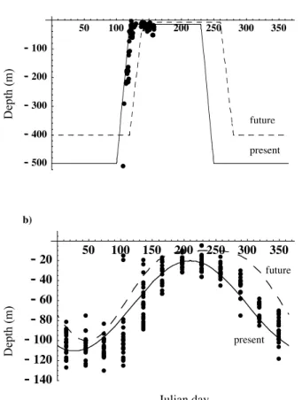
The seasonal mixed layer was modeled either by a piecewise linear function (NABE site) or by a power sine function approximating the seasonal mixed layer dynam-ics (OSP). Both functions closely match the observed mixed layer depth dynamdynam-ics (Figs. 1a and b). Using the sine function for the North Atlantic site gave qualitatively similar results. Irradiance (daily average PAR, 400–700 nm) at the top of the

atmo-15

sphere for the given latitudes was modeled as in Brock (1981) and the daily PAR reaching the ocean’s surface was calculated as in Evans and Parslow (1985). The model equations were solved using Mathematica software (Wolfram Research).

2.1.3 Taxonomic differences in competitive abilities

Using the average parameters for each taxonomic/functional group (Table 2), we

de-20

termined the competitive abilities of all groups for major nutrients (nitrate, ammonium,

phosphate and iron). The competitive abilities were characterized using the R*

con-cept, where the best competitor has the lowestR*, the resource concentration at which

(13)

BGD

3, 607–663, 2006

communities

E. Litchman et al.

Title Page

Tables Figures

◭ ◮

Back Close

Full Screen / Esc

EGU

following:

R∗

i =

kiµmax,iQmin,imi

Vmax,i(µmax,i−mi)−µmax,iQmin,imi

(13)

Symbol definitions and values for each taxonomic group are listed in Table 2. According to this expression, taxonomic groups differ in their competitive abilities for major

nutri-ents: diatoms are generally good nutrient competitors, having lowR*s for all nutrients,

5

and dinoflagellates are poor nutrient competitors (Table 4). As theR*s depend on

mor-talities, we used non-grazing mortalities from the model (Table 2) to estimate groups’ competitive abilities. For the given mortalities, coccolithophores and diatoms are the better competitors for nitrate, coccolithophores are superior competitors for phosphate,

and prasinophytes are effective competitors for ammonium but poor competitors for

10

nitrate (Table 4). Based on the chosen Fe utilization parameters, coccolithophores (E. huxleyi) are the best Fe competitors, followed by dinoflagellates and diatoms and

prasinophytes having poorer competitive abilities for Fe. In addition to R*s of each

group, other eco-physiological characteristics, such as light requirements and grazer resistance, contribute to the ecological success of individual species and functional

15

groups. A poor competitor for inorganic nutrients may still persist in the community due to its high grazer resistance.

2.2 Modern ocean verification

The model was tested using two data sets from sites that differ considerably in

phyto-plankton community structure and patterns of seasonal succession. The North

At-20

lantic region, typified by the JGOFS North Atlantic Bloom Experiment site (NABE,

47◦N 20◦W) exhibits pronounced seasonality with a spring bloom of diatoms often

followed by a non-diatom bloom (Joint et al., 1993). Nutrients are depleted season-ally (Longhurst, 1998). The North Pacific region, represented by the Ocean Weather

Station Papa (OSP, 50◦N 145◦W), exhibits much less seasonality in phytoplankton

25

(14)

nu-BGD

3, 607–663, 2006

communities

E. Litchman et al.

Title Page

Tables Figures

◭ ◮

Back Close

Full Screen / Esc

EGU

trients. OSP resides in a High Nutrient Low Chlorophyll (HNLC) region of the global ocean (Longhurst, 1998; Harrison et al., 1999). Iron (Fe) is likely an important limiting nutrient in this region (Boyd and Harrison, 1999; Tsuda et al., 2003). These two re-gions of the world ocean are important components in the global carbon cycle and their

phytoplankton community structure profoundly affects the magnitude of the carbon flux

5

(Hanson et al., 2000).

The NABE data that we used to validate our model were taken from the JGOFS

web site (http://usjgofs.whoi.edu/jg/dir/jgofs/nabe) and the University Corporation for

Atmospheric Research (UCAR) web site (http://dss.ucar.edu/datasets/ds259.0/). The

data for OSP were also obtained from the UCAR web site (Kleypas and Doney, 2001).

10

The goal of the verification procedure was both qualitative and quantitative agree-ment with the data, with an emphasis on the presence or absence and relative abun-dance of certain functional/taxonomic groups, the pattern of seasonal succession, and nutrient dynamics. We describe model results for the two sites. The results reported represent model behavior after it reaches a year-to-year equilibrium, i.e., the pattern is

15

identical from year to year.

2.3 Modern ocean parameter sensitivity analysis

We explored how model behavior depends on the model parameters and determined ranges of parameters that produce adequate ecosystem dynamics at each site. A sin-gle parameter was altered at a time (Fasham et al., 1990) according to the following

20

scheme: the parameter space was scanned to the left and to the right from the orig-inal value (from 0 to 3 times the initial parameter value) using the bisection method (Press et al., 1992). For each new value of the parameter, the model was run to an equilibrium annual cycle that was compared to the model dynamics with the original parameter value. As we are interested in a number of model results including

pres-25

(15)

BGD

3, 607–663, 2006

communities

E. Litchman et al.

Title Page

Tables Figures

◭ ◮

Back Close

Full Screen / Esc

EGU

with the changed parameter. We summarize these criteria in Table 5. The runs and, consequently, the corresponding parameter values that met all the criteria from Table 5 were considered acceptable. The criteria for model assessment were constrained by the data where possible (Table 5), with better constraints for OSP, as there are multi-year data available for this site. For example, the lower and upper bounds for average

5

yearly concentration of Si, N and chlorophyll were determined by the lowest and the highest yearly averages from the time series data for OSP.

2.4 Global change scenarios

We considered the following aspects of global change that will likely affect marine

phy-toplankton communities: global warming-induced changes in mixed layer depth and the

10

duration and timing of the vertical stratification period, shifts in the N:P ratios in deep water (increase in N concentration or a decrease in P concentration) and changes in iron deposition (both increase and decrease). We applied five hypothetical scenarios to the communities of the two sites we considered here: North Atlantic (NABE) and Subarctic North Pacific (OSP).

15

2.4.1 Change in the mixed layer dynamics

A future increase in atmospheric greenhouse gases will likely change ocean mixed layer dynamics (Manabe et al., 1991; Sarmiento et al., 1998). We constructed

sce-narios for these changes in mixing dynamics owing to increases in atmospheric CO₂

concentration based on simulations of the global coupled atmosphere-ocean-ice model

20

described in Russell et al. (1995) and Miller and Russell (1997). Two 150-year model simulations were used in this study. The first was a control simulation for the present climate in which atmospheric greenhouse gases (GHG) are fixed at 1950 levels. The second was a greenhouse gas simulation in which carbon dioxide concentrations in-crease at the observed rate between 1950 and 1990 and then inin-crease at a rate of

25

(16)

BGD

3, 607–663, 2006

communities

E. Litchman et al.

Title Page

Tables Figures

◭ ◮

Back Close

Full Screen / Esc

EGU

as the basis for constructing scenarios of changes in mixed layer dynamics at the two sites. It is important to note that because global climate models generally have limited ability to predict changes at single grid boxes, the scenarios here are only represen-tative of possible future outcomes. For the increasing GHG scenario, the model sea surface temperature increased at both sites: 1.5 degrees in winter and 0.85 degrees in

5

summer for the Atlantic site and 1 degree in winter and 0.6 degree in summer for the Pacific site. For the GHG simulation the surface wind stress at both sites is higher than in the control simulation from December to May, the same in June and July, and lower in the fall.

Based on the climate model simulations, scenarios for annual cycles of mixed-layer

10

depth at the two sites are constructed and shown in Figs. 1a and b. Qualitatively, the shoaling of the mixed layer depth at the Atlantic Ocean site occurs about a month later and lasts longer for the GHG scenario due to changes in the wind stress. The mixing depth is slightly shallower in the summer. At OSP the mixed layer depth decreases ear-lier in the spring and stays shallower longer under the GHG scenario. A decrease in the

15

mixed layer depth at a rate of about 63 m/century has been already observed at OSP due to warmer temperatures (Freeland et al., 1997; Woody et al., 1999). We quanti-fied these general scenarios as shown in Fig. 1 and applied them to the phytoplankton community model at both sites.

2.4.2 Change in the deep water N:P ratio

20

Small increases in the deep water N:P ratios over several decades have been reported

at different parts of the world ocean, including North Atlantic and North Pacific oceans

(Pahlow and Riebesell, 2000; B ´ethoux et al., 2002), although the magnitude and the causes for such shifts are in dispute (Gruber et al., 2000). We increased the deep water N:P ratios at both sites by a) doubling the N concentration or b) halving the P

25

(17)

BGD

3, 607–663, 2006

communities

E. Litchman et al.

Title Page

Tables Figures

◭ ◮

Back Close

Full Screen / Esc

EGU

2.4.3 Change in iron (Fe) deposition

Increased global mean temperatures will likely alter patterns of atmospheric Fe depo-sition (Fung et al., 2000). Higher temperatures may lead to higher precipitation and a subsequent decrease in the dust flux, or may increase soil aridity and enhance the aeolian flux. The magnitude and sign of the change are hard to predict because of

5

numerous feedbacks and uncertainties in future land use practices (Fung et al., 2000;

Ridgwell, 2002). We explore the effects of both doubled and halved Fe deposition

at both sites on phytoplankton community structure. The change in Fe deposition is modeled by changing the deep water Fe concentration, similar to Fennel et al. (2003).

2.5 Robustness of the future scenario predictions

10

The global change scenario predictions may depend idiosyncratically on a given

com-bination of parameter values. It is possible that a different combination of parameters

with each of these parameters within its acceptable range may produce a different

out-come under global change scenarios and thus decrease the reliability of predictions. This problem is especially acute in models with multiple functional groups, as limited

15

data exist to parameterize such parameter-rich models. To increase the robustness of our model predictions, we used a Monte Carlo approach where the model was run un-der present conditions with all parameters randomly selected from a predefined range and the model outcome was tested against the chosen criteria (Table 5) to determine how well a given parameter combination predicted modern ecosystem dynamics. This

20

allows us to decrease the effects of uncertainty of model parameterizations. For

param-eters with a known distribution (based on our database), we used the 25th and 75th percentiles to define the sampling range. For the rest of the parameters the ranges

were defined as the parameter value±1/2 of its value. If the model outcome and,

con-sequently, the given parameter combination were deemed acceptable for the modern

25

(18)

BGD

3, 607–663, 2006

communities

E. Litchman et al.

Title Page

Tables Figures

◭ ◮

Back Close

Full Screen / Esc

EGU

each group of phytoplankton, average nutrient concentrations, timing and magnitude of the diatom bloom (for NABE only) were stored. A total of 100 random parameter combinations that produced acceptable present day model outcomes were run under global change scenarios for each site. For each key variable, the results from each global change scenario were compared with the present day values obtained with the

5

given parameter combination and reported as percent change. To assess the variation in model predictions, we report the 50th, as well as 5th, 25th, 75th and 95th percentiles of the prediction range for 100 acceptable runs.

3 Results

3.1 Modern ocean verification

10

3.1.1 North Atlantic Ocean

At NABE, a typical seasonal succession pattern consists of low phytoplankton abun-dance in winter, a spring bloom of diatoms with a subsequent bloom of non-diatom

phy-toplankton, often coccolithophorids (Emiliania huxleyi) and other flagellates (Lochte et

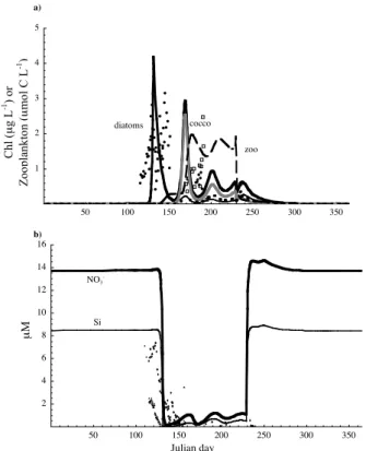
al., 1993; Savidge et al., 1995; Broerse et al., 2000). The model predicts this seasonal

15

succession pattern with the diatom bloom in spring followed by the coccolithophore and flagellate blooms later in the summer (Fig. 2a). All three groups coexisted stably over an annual cycle. This pattern agrees with the JGOFS data and was also predicted by the model of Gregg et al. (2003). The magnitude of the blooms also agrees with the JGOFS data for NABE (Fig. 2a). The nutrient drawdown is highly seasonal, with

20

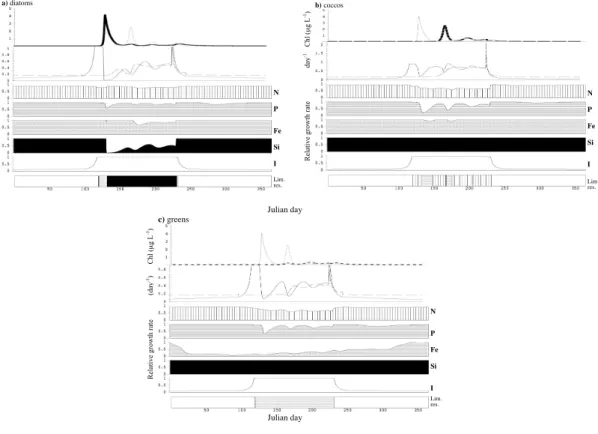
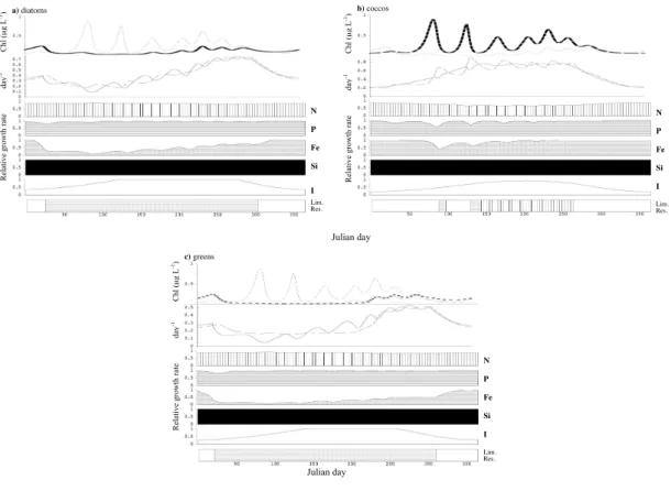
nitrate, P and Si becoming depleted in the summer (Fig. 2b). The growth rate of each phytoplankton group in the spring greatly exceeds its mortality rate (Fig. 3, panel 2).

The identity of the most limiting resource changes throughout the season and differs

among groups (Fig. 3), thus justifying post hoc the need for a multi-nutrient approach. All groups are light-limited in winter, early spring and fall, when mixed layer is deep

(19)

BGD

3, 607–663, 2006

communities

E. Litchman et al.

Title Page

Tables Figures

◭ ◮

Back Close

Full Screen / Esc

EGU

(Fig. 3). The increases of diatom and later coccolithophore and prasinophyte popula-tions are possible when light-limited growth rate exceeds mortality (Fig. 3). During the stratified period, diatoms are limited mostly by Si with brief periods of nitrogen and iron limitation, and the spring diatom bloom is terminated due to depletion of Si (Figs. 2 and 3). Growth of coccolithophorids is limited by either P or N during the stratified period

5

(Fig. 3b) and prasinophyte growth is limited by Fe and controlled by increasing grazer population and later on by the deepened mixed layer and decreased light availability (Fig. 3c). Zooplankton abundance is also highly seasonal, with extremely low density in the winter and higher concentrations associated with phytoplankton blooms (Fig. 2a).

3.1.2 North Pacific Ocean

10

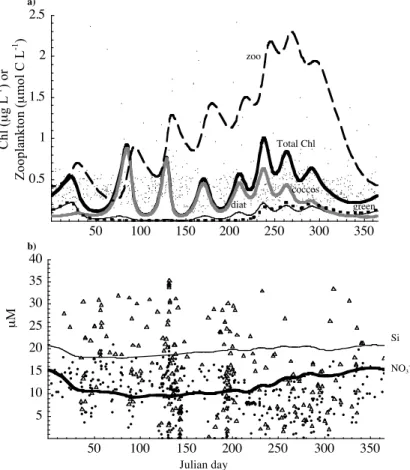
The observed community structure and seasonal patterns are different at OSP from

NABE. The biomass of phytoplankton does not exhibit high amplitude seasonal fluctu-ations. In contrast with the North Atlantic, diatoms do not reach high densities because of severe Fe limitation (Tsuda et al., 2003). The eukaryotic phytoplankton commu-nity consists primarily of prymnesiophytes, including coccolithophores, and diatoms

15

and prasinophytes. Among coccolithophores,E. huxleyi is the most abundant species

(Muggli and Harrison, 1996) and can reach at least 40% of total phytoplankton biomass (Lam et al., 2001). A characteristic feature of OSP is that prasinophytes contribute sig-nificantly to the total cell abundance (Boyd and Harrison, 1999). Coccolithophores can be abundant as well and were previously underestimated (Harrison et al., 2004).

20

The predicted dynamics of the phytoplankton community in our model agrees well with observations. Diatoms, coccolithophores and prasinophytes coexist stably at this site (Fig. 4a). In contrast to NABE site, over the yearly cycle, total mortality closely follows growth rate for all functional groups (Fig. 5, panel 2). Diatoms do not bloom and their biomass does not reach high values (Figs. 4a and 5a). According to the

25

(20)

BGD

3, 607–663, 2006

communities

E. Litchman et al.

Title Page

Tables Figures

◭ ◮

Back Close

Full Screen / Esc

EGU

grazing. Prasinophytes are limited by light and Fe and controlled by grazing (Fig. 5c). Total phytoplankton biomass at this site exhibits little seasonality and does not attain values as high as in the North Atlantic (Fig. 4a). There is, however, some seasonality in the abundances of individual groups, with diatoms and prasinophytes achieving higher densities in late fall and winter and coccolithophores in the spring and summer (Figs. 4a

5

and 5). Oscillations in phytoplankton and zooplankton biomass are likely

predator-prey cycles and similar oscillations were observed at this site (see OSP data athttp:

//dss.ucar.edu/datasets). Nitrate and Si remain high throughout the year in the model, which agrees with observations (Fig. 4b). Microzooplankton biomass varies ca. four-fold over the season (Fig. 4a), which also corresponds to observations (Boyd et al.,

10

1999).

3.2 Modern ocean parameter sensitivity analysis

The results of the sensitivity analysis are given in Table 6. Different parameters have

different sensitivities; some parameters have a large effect on the model outcome and,

hence, narrow ranges that produce acceptable model behavior (Table 5) and others

15

do not. Sensitive parameters include phytoplankton maximum growth rates (µmax),

minimum Fe quotas (QFe_min), Si content of diatoms (QSi), maximum uptake rates for

nitrate (VN_max), P (VP_max), Fe (VFe_max), half-saturation constants for uptake of P (kP), Fe (kFe), light-half saturation constants (kI), phytoplankton mortalities (m), group-specific

zooplankton grazing preferences (c), background light attenuation (a_bg), zooplankton

20

maximum grazing rate (g), half-saturation constant for zooplankton grazing (kz),

phy-toplankton to zooplankton conversion efficiency (cz) and zooplankton mortality (mz).

Variation in other parameters within the set limits did not affect model results

consid-erably, i.e., the chosen criteria of the model results (Table 5) were met over the whole parameter range.

25

Another important result that emerged from the sensitivity analysis is that the

(21)

BGD

3, 607–663, 2006

communities

E. Litchman et al.

Title Page

Tables Figures

◭ ◮

Back Close

Full Screen / Esc

EGU

parameters and the acceptable parameter ranges differed between NABE and OSP

(Table 5). For example, maximum growth rates are sensitive parameters at both sites, but the ranges are tighter for NABE (Table 6), as at this site phytoplankton have peri-ods of high growth and thus model behavior depends strongly on the maximum growth rate values, while at OSP such periods are shorter due to severe Fe limitation

through-5

out the year. Also, light is an important factor at NABE as it determines the timing of the spring diatom bloom, and, consequently, model behavior is sensitive to changes in

half-saturation constants for light-dependent growth (kI) and background light

attenua-tion (abg) (Table 6). At OSP, Fe utilization parameters had large influence on the model

outcome as evident from the narrow acceptable ranges for those parameters (Table 6).

10

At both sites, grazing parameters (grazing preference for each group,ci, zooplankton

maximum grazing rate,g, half-saturation constant for grazing,kz and phytoplankton to

zooplankton conversion efficiency,c_z) had a large effect on model behavior, but the ac-ceptable ranges of those parameters were narrower for OSP, thus indicating a relatively larger importance of grazing at this site.

15

3.3 Global change scenarios

Here we report the results of an ensemble of one hundred runs with different

param-eter combinations that produced adequate modern day dynamics at each site. This increases the robustness of our predictions by diminishing their dependence on a par-ticular parameter combination.

20

3.3.1 Change in the mixed layer dynamics

At NABE the diatom bloom is predicted to occur later in the year, following later strat-ification, and the magnitude of the bloom will likely decrease (Table 7). The average yearly biomass of diatoms is, however, similar to the present day. In contrast, average biomass of prasinophytes and especially, zooplankton, increases significantly. The

av-25

(22)

BGD

3, 607–663, 2006

communities

E. Litchman et al.

Title Page

Tables Figures

◭ ◮

Back Close

Full Screen / Esc

EGU

parameter combinations it could decrease (Table 7). Nutrients remain at low levels for a larger part of the year due to prolonged stratification. At OSP in the North Pacific, a longer stratification period with a shallower mixed layer depth (Fig. 1b) will lead to an increase in average nitrate and silicate, average biomass of diatoms and prasino-phytes, and consequently, of average chlorophyll. Average zooplankton biomass will

5

also increase significantly (Table 7). The average yearly biomass of coccolithophores will likely be similar to the present day.

3.3.2 Change in the deep water N:P ratio

In the North Atlantic, the increase of the deep water N:P ratio (by decreasing P

concen-tration by half, from 1 to 0.5µM P) in deep water leads to lower average coccolithophore

10

biomass, with no major change in the average biomass of green algae and diatoms, but a smaller spring diatom bloom (Table 7). Average chlorophyll concentration and zooplankton biomass will likely decline (Table 7). In the North Pacific, the increase

in N:P deep water ratio by halving P concentration (from 2.5 to 1.25µM) has a much

smaller effect on ecosystem dynamics compared to the North Atlantic site: the

mag-15

nitude of changes in key variables is much smaller (Table 7). The phytoplankton and zooplankton dynamics retain pronounced seasonality at NABE and low seasonality at OSP. An increase in the N:P deep water ratios by increasing nitrate concentration

(2-fold increase) does not have a large effect at the two sites, the community composition

and dynamics remain similar to the present day (Table 7).

20

3.3.3 Change in iron (Fe) deposition

Doubling the Fe concentration at NABE (from 1 to 2 nM) leads to a significant increase in average biomass of prasinophytes, no change in diatom biomass and a decrease in coccolithophore average biomass (Table 7). The average chlorophyll concentration and zooplankton biomass increase. Halving the Fe concentration at NABE (from 1 to

25

(23)

combi-BGD

3, 607–663, 2006

communities

E. Litchman et al.

Title Page

Tables Figures

◭ ◮

Back Close

Full Screen / Esc

EGU

nations prasinophytes get excluded due to increased iron limitation under this scenario. In contrast, average biomass of coccolithophores increases significantly and diatom biomass as well as the magnitude of spring diatom peak may decline slightly. Total chlorophyll concentration decreases, as well as the microzooplankton biomass.

The doubling the Fe concentration at OSP consistently increases average biomass of

5

diatoms, prasinophytes, average chlorophyll concentration and zooplankton biomass. Coccolithophores decline under this scenario. Nutrients (e.g., N, Si) are utilized more

efficiently and their average concentration decreases (Table 7). Halving the Fe

concen-tration leads to a decline in diatoms, prasinophytes, average chlorophyll and zooplank-ton biomass. For some parameter combinations, prasinophytes are excluded from the

10

community. Coccolithophores increase in abundance. Due to severe Fe limitation, uptake of macronutrients is lower, leading to their higher average concentrations (Ta-ble 7).

4 Discussion

Our mechanistic phytoplankton community model with minimal physics captures the

15

principal characteristics of phytoplankton dynamics over the annual cycle. The model

is capable of reproducing the distinctly different patterns of abundance and succession

at two characteristic sites of the ocean. Although we aimed at developing a simple model, we included multiple nutrients that can limit phytoplankton growth, e.g., P, which is often omitted from the ocean phytoplankton models. There are compelling reasons

20

to include P into the models of marine phytoplankton. Our data compilation shows

that major taxonomic groups differ in their competitive abilities not only for N but P

as well. Therefore, including growth dependence on P allows for better separation

of different functional groups. Moreover, some regions of the ocean are P-limited at

present and the extent of such areas may increase in the future (Ammermann et al.,

25

(24)

BGD

3, 607–663, 2006

communities

E. Litchman et al.

Title Page

Tables Figures

◭ ◮

Back Close

Full Screen / Esc

EGU

phytoplankton stoichiometry and carbon and nutrient drawdown ratios (Klausmeier et al., 2004), observed at these sites (Bury et al., 2001).

As we aimed at modeling phytoplankton community structure, we did not include some key ecosystem variables such as bacteria or dissolved organic matter. Instead, we concentrated on adequately describing major ecological controls of the main

func-5

tional groups of eukaryotic phytoplankton, such as nutrients, light and grazing. The community composition and succession are sensitive not only to the levels and ratios of resources but to grazing parameters as well. It is likely that models with greater taxo-nomic resolution of phytoplankton are more sensitive to grazing parameter values than models considering only total chlorophyll dynamics. A high sensitivity to grazing

param-10

eters has been observed in other ecosystem models (see references in Pe ˜na, 2003) and underscores the importance of quantifying grazer impact on community structure. A systematic parameter sensitivity analysis revealed other sensitive parameters and the ranges that produce acceptable model behavior. Where possible, we compared the acceptable ranges of parameters obtained in the sensitivity analysis with

parame-15

terizations from other models of multiple phytoplankton functional groups (e.g., Moore et al., 2002; Gregg et al., 2003). In many cases those parameterizations fall within our estimated ranges (e.g., maximum growth rates).

Predicting phytoplankton community patterns under future scenarios is uncertain

due to difficulties in parameterization and may depend on model structure and

pa-20

rameter combinations. We explored this uncertainty using Monte Carlo techniques where future scenarios are run with multiple parameter combinations that produced acceptable modern day dynamics. To our knowledge, this is the first such attempt to reduce the uncertainty of predictions in a model with multiple phytoplankton functional groups. Our future predictions are based on randomly chosen parameter sets that

25

(25)

BGD

3, 607–663, 2006

communities

E. Litchman et al.

Title Page

Tables Figures

◭ ◮

Back Close

Full Screen / Esc

EGU

sites (Table 7). Similarly, average zooplankton biomass will likely increase significantly under the predicted changes in MLD dynamics at both sites. The magnitude of change in key variables is, however, more dependent on the parameter combinations.

The competitive rankings of major taxonomic groups based on experimental data and our model predictions are consistent with the observed patterns of the

commu-5

nity structure in the ocean. Diatoms grow at lower light, have high maximum growth rates and, as our results suggest, are good N competitors. These traits enable them to increase ahead of other groups as irradiance increases due to spring increase in solar declination and shoaling of the mixed layer (Sverdrup, 1953). A later onset of stratification delays the occurrence of spring diatom bloom. With a shallower mixed

10

layer depth, light availability increases, thus, diminishing the competitive advantage of diatoms. Consequently, as predicted by the model, the magnitude of the spring diatom bloom decreases with longer stratification period under the global change scenario. At the same time, coccolithophores and prasinophytes, having higher half-saturation con-stants for light-dependent growth, are likely to increase under this scenario at NABE

15

(Table 7). Stimulation of coccolithophores by prolonged stratification has been ob-served in the Bering Sea, where an unusually long stratification period in 1997 and 1998 had lead to massive coccolithophore blooms (Napp and Hunt, 2001; Iida et al., 2002). Recent global satellite data analysis also showed strong association of

coccol-ithophore blooms with highly stratified conditions (Iglesias-Rodr´ıgues et al., 2002).

20

As our analysis suggests, prasinophytes are relatively poor nitrate competitors (Ta-ble 4) and, consequently, they can be abundant where nitrate is not depleted (HNLC regions). For example, at OSP (HNLC region) high prasinophyte abundance is ob-served (Varela and Harrison, 1999) and predicted by our model. According to the available data on Fe utilization, coccolithophores are good Fe competitors and,

con-25

sequently, increase under decreased Fe deposition, while diatoms and prasinophytes

decline. Our predicted long-term effects of the Fe concentration increase such as the

increase of diatoms in the HNLC areas and a more efficient nutrient drawdown agree

(26)

BGD

3, 607–663, 2006

communities

E. Litchman et al.

Title Page

Tables Figures

◭ ◮

Back Close

Full Screen / Esc

EGU

et al., 2003) and with the predictions of other models (Moore et al., 2004). Other predictions are less intuitive, such as the decrease of coccolithophores at both sites under increased Fe deposition. Increased Fe availability decreases the importance of Fe competition and allows poorer Fe competitors (diatoms and prasinophytes) to domi-nate. Our results on community shifts under various Fe deposition scenarios are greatly

5

dependent on the group-specific Fe utilization parameters. More experimental data on Fe-dependent growth and uptake by major phytoplankton groups, e.g., prasinophytes, are critical for generating credible predictions.

Changes in nutrient ratios in deep waters have been observed in various parts of the ocean. For example, in the Mediterranean Sea the Si:P ratio has declined due

10

to an anthropogenic increase in phosphate input over the last few decades (B ´ethoux et al., 2002). Physical mixing brings nutrients at altered ratios to the upper ocean. Consequently, changes in ambient nutrient ratios may shift community composition

due to differential requirements and competitive abilities of the phytoplankton functional

groups for major nutrients.

15

Based on our literature survey, it appears that major functional groups are

signifi-cantly different in their nutrient utilization patterns and competitive abilities. We have

included these differences in the model. However, a number of parameters that are

likely to be group-specific (light-attenuation coefficients, ammonium inhibition

con-stants, maximum grazing rates and phytoplankton to zooplankton conversion effi

cien-20

cies) were assumed to be the same for all groups. Possible refinements of the model can include a group-specific choice of the above-mentioned parameters or including other physiological processes such as photoinhibition. This will allow for an even

greater separation of different functional groups. In addition, nitrogen fixers

(cyanobac-teria) must be included to apply the model to other sites (e.g., tropics and subtropics)

25

in the global ocean. They can also be explicitly modeled in the future versions of this

model to more fully explore the effects of warming at NABE and OSP, as increased

(27)

BGD

3, 607–663, 2006

communities

E. Litchman et al.

Title Page

Tables Figures

◭ ◮

Back Close

Full Screen / Esc

EGU

the indirect effects of global warming on the phytoplankton community structure but

such dependence may also be included in the future versions of the model. In our model each functional group is represented by one composite “species” with the key parameter values averaged over a range of species. Thus, the model is capable of describing only the “average” behavior of each group. Future refinements could

explic-5

itly model within-group variability (e.g., size-related differences) by including more than one compartment for each taxonomic group.

Our study indicates that changes in mixed layer dynamics may change both the tim-ing and magnitude of the phytoplankton blooms as well as community composition. Significant changes in community composition due to climatic alterations are being

ob-10

served in the world ocean and are referred to as the “domain shift hypothesis” (Karl et al., 2001). A disappearance of individual species or functional groups as predicted in

some global change scenarios may have a dramatic effects on community and

ecosys-tem dynamics (Berlow, 1999). The later timing and smaller magnitude of the diatom bloom in the North Atlantic under the increased greenhouse gas scenario may have

15

profound consequences for higher trophic levels, e.g., the survival of larval stages of the commercial fish populations. A recent study showed that the timing of the phy-toplankton bloom accounted for 89% of variance in the survival of larval haddock in the North Atlantic, where a 5-week delay in spring bloom decreased the fish survival index more than 5-fold (Platt et al., 2003). Historic variation in the mixed layer

dy-20

namics and consequent changes in primary productivity have been shown to affect

commercial fisheries in the Pacific as well (Chavez et al., 2002). The scenarios for changes in mixed layer dynamics are based on simulations of a global climate model and should be considered only as representative of possible future outcomes. Global models are still not very reliable for making predictions for changes at specific sites.

25

Predicting changes in mixed layer depth are particularly difficult because they require

(28)

BGD

3, 607–663, 2006

communities

E. Litchman et al.

Title Page

Tables Figures

◭ ◮

Back Close

Full Screen / Esc

EGU

eco-physiological traits induced by climate change. Such changes are not considered by our model, as they are poorly known. They, however, may set ecosystem dynamics

on trajectories very different from the ones predicted by our model.

Increased concentration of greenhouse gases may alter stratification patterns and reduce Fe deposition. Our results indicate that these key consequences of global

5

change may shift competitive interactions among phytoplankton and decrease diatom

distribution and abundance in different parts of the world ocean. Decreased diatom

abundance may in turn decrease efficiency of carbon export production (carbon

se-questration) and increase CO2 in the atmosphere, thus creating a positive feedback

between phytoplankton community structure and climate change. The predicted shift

10

toward dominance by coccolithophores under some global change scenarios would

enhance biocalcification and thus significantly changepCO2 (Doney et al., 2000) and

global albedo (Tyrrell et al., 1999). The predicted increase in prasinophyte abundance may also significantly alter carbon sequestration patterns and trophic interactions by stimulating microzooplankton growth. Human-induced changes in physico-chemical

15

ocean characteristics almost certainly will alter the structure of phytoplankton

commu-nities and thus have a profound effect on ecosystem structure and global

biogeochem-ical cycles. Using composite characteristics of major taxonomic groups based on the extensive experimental data compilation may allow for meaningful parameterizations of phytoplankton community models that can then be used for qualitative predictions

20

amenable to mechanistic interpretation.

Appendix A

References used to obtain data for Table 2

Bhovichitra, M. and Swift, E.: Light and dark uptake of nitrate and ammonium by

25

large oceanic dinoflagellates: Pyrocystis noctiluca, Pyrocystis fusiformis, and

(29)

BGD

3, 607–663, 2006

communities

E. Litchman et al.

Title Page

Tables Figures

◭ ◮

Back Close

Full Screen / Esc

EGU

Bienfang, P. K.: Steady-state analysis of nitrate-ammonium assimilation by phyto-plankton, Limnol. Oceanogr., 20, 402–411, 1975.

Caperon, J. and Meyer, J.: Nitrogen-limited growth of marine phytoplankton. 2. Up-take kinetics and their role in nutrient limited growth of phytoplankton, Deep-Sea Res., 19, 612–632, 1972.

5

Carpenter, E. J. and Guillard, R. R. L.: Intraspecific differences in nitrate

half-saturation constants for three species of marine phytoplankton, Ecology, 52, 183–185, 1971.

Cembella, A. D., Antia, N. J., and Harrison, P. J.: The utilization of inorganic and organic phosphorus compounds as nutrients by eukaryotic microalgae: a

multidisci-10

plinary perspective: part 1, CRC Crit. Rev. Microbiol., 10, 317–391, 1984.

Cochlan, W. P. and Harrison, P. J.: Kinetics of nitrogen (nitrate, ammonium and urea)

uptake by picoflagellate Micromonas pusilla (Prasinophyceae), J. Experimental Mar.

Biology and Ecology, 153, 129–141, 1991.

Conway, H. L. and Harrison, P. J.: Marine diatoms grown in chemostats under silicate

15

or ammonium limitation. IV Transient response ofChaetoceros debilis,Skeletonema

costatum and Thalassiosira gravida to a single addition of the limiting nutrient, Mar. Biology, 43, 33–43, 1977.

Davidson, K. and Gurney, W. S. C.: An investigation of non-steady-state algal growth. II. Mathematical modelling of co-nutrient-limited growth, J. Plankton Res., 21, 839–858,

20

1999.

Deane, E. M. and O’Brien, R. W.: Uptake of phosphate by symbiotic and free-living dinoflagellates, Archives of Microbiology, 128, 307–310, 1981.

Eppley, R. W. and Coatsworth, J. L.: Nitrate and nitrite uptake byDitylum brightwellii:

kinetics and mechanisms, J. Phycology, 4, 151–156, 1968.

25

Eppley, R. W. and Renger, E. M.: Nitrogen assimilation of an oceanic diatom in nitrogen-limited continuous culture, J. Phycology, 18, 534–551, 1974.