METHODS FOR THE ASSESSMENT OF PERFORMANCE
INDICATION MEASURES AT AMAKOM INTERSECTION AND
THEIR APPLICATION IN MICRO SIMULATION MODELING
Emmanuel Kwesi Nyantakyi1, Prince Appiah Owusu2, Julius Kwame Borkloe3 1, 2, 3 Department of Civil Engineering, Kumasi Polytechnic, P.O. Box 854, Kumasi-Ghana Received 20 March 2013; accepted 2 July 2013
Abstract: Signalized intersections are vital nodal points in a transportation network and their efficiency of operation greatly influences the entire network’s performance. Traffic simulation models have been widely used in both transportation operations and traffic analyses because simulation is safer, less expensive, and faster than field implementation and testing. This study assessed performance indication measures at Amakom intersection using micro simulation models in Synchro/SimTraffic. Traffic, geometric and signal control data including key parameters with greatest impact on the calibration process were collected on the field. At 5% significant level, the Chi square test and t-test analyses revealed that headway had a strong correlation with saturation flow compared to speed for both field and simulated conditions. It was concluded that changes in phasing plan with geometric improvement would improve upon the intersection’s level of service.
Keywords:performance indication measures, signalized intersection, Synchro/SiMTraffic, transportation network performance, traffic geometric, signal control.
1 Corresponding author: [email protected]
1. Introduction
In general, simulation is defined as dynamic representation of some part of the real world achieved by building a computer model and moving it through time (Drew, 1968). Computer models are widely used in traffic and transportation system analysis. The use of computer simulation started when D.L. Gerlough published his dissertation: “Simulation of freeway traffic on a general-purpose discrete variable computer” at the University of California, Los Angeles, in 1955 (Kallberg, 1971). From those times, computer simulation has become a widely used tool in transportation engineering
w it h a v a r iet y of appl ic at ion s f rom scientific research to planning, training and demonstration.
Previous studies by BCEOM and ACON Report (2004) on the performance of the intersection attributed the congestion critical capacity, intersection controls and abuse to motorists and/or pedestrians. It was concluded that most of the sections on the 24th February road have their capacities approaching critical (v/c ratio > 0.6) and that this contributes in part to the congestion which results in delay and subsequent poor performance of the road. It was therefore recommended that this section of the 24th February road will be highly critical between 2004 and 2009.
As part of the recommendations, the report proposed to improve upon the signalization and capacity at the intersection through; revision of signal timing, phasing plan and inclusion of exclusive NMT phase and removal of illegal taxi rank at the filling station on the Asawasi leg at A makom intersection (BCEOM and ACON Report, 2004). In the study although the micro si mu l at ion Sy nc h ro/Si mTra f f ic w a s reportedly used for the analysis, the models were not calibrated. Even though some of the recommendations have been implemented at the intersection, long queues and frequent delays st i l l persist dur ing pea k hour conditions (BCEOM and ACON Report, 2004). Since in the application of micro simulation tools, one major step is calibration before the prediction can be said to mimic site conditions, this needs to be checked. Also micro simulation tools application is relatively new in Ghana and the procedures for calibration, and application in modeling is not very well understood by practicing engineers. Outputs of micro simulation models are useful to traffic engineer to identify existing problems and come out with interventions. A micro simulation model in Synchro is software that makes use of limited
data by trying to mimic the present traffic situation, which is then used in forecasting the future traffic conditions based on the present. This study seeks to contribute to the knowledge base in the area by calibrating the Synchro/SimTraffic models and using the concept to predict the performance of the Amakom intersection. The study therefore assessed performance indication measures at the Amakom intersection using micro simulation models in Synchro/SimTraffic.
2. Methodology
2.1. Calibration of Synchro for Site
Condition
T he ca l ibration procedure employed Turley (2007) approach by first selecting the intersection, collecting required input data for the Synchro model and collecting calibration data. These were then followed by comparing calibration data with simulated results from the field and finally calibrating the model.
2.2. Site Selection and Description
traffic light and 700 m away from labour roundabout. The intersection has four legs with one approach/entry and exit through lanes on each leg of the minor road (Yaa Asantewaa road), and two approach/entry
and exit through lanes on the 24th February road. It is the intersection of a Principal arterial and a Collector road. Fig. 1 is the map of Kumasi showing the intersection under study.
Fig. 1.
Map of Kumasi Showing Amakom Intersection on the 24th February Road
Source: Department of Urban Roads, Ghana
Fig. 2.
Geometry of 24th February / Yaa Asantewaa Road Intersection
2.3. Basic Theoretical Background
The concept of “car-following” describes the detailed movement of vehicles proceeding close together in a single lane. This theory is based on the assumption that each driver reacts in some specific fashion to a stimulus from the vehicle ahead of him.
One of the oldest and most well known cases of the use of simulation in theoretical research is the “car-following” analysis based on the Generalized General Motors (GM) models. In these models a differential equation governs the movement of each vehicle in the platoon under analysis (Gerlough and Huber, 1975). Car-following, like the intersection analysis, is one of the basic equations of traffic f low theory and simulation, and the analysis has been active after almost 40 years from the first trials (McDonald et al., 1998).
The car-following theory is of significance in microscopic traffic flow theory and has been widely applied in traffic safety analysis and traffic simulation (Luo et al., 2010; Tordeux et al., 2010). There have been many car-following models in the past 60 years, and the models can be divided into two categories. One is developed from the viewpoint of traffic engineering and the other is based on statistical physics. From the perspective of traffic engineers (Brackstone and McDonald, 1999), car-following models can be classified as stimulus-response models (Gazis et al., 1961; Newell, 1961), safety distance models (Gipps, 1981), psycho-physical models (Wiedemann, 1974), and artificial intelligence models (Kikuchi and Chakroborty, 1992; Wu et al., 2000).
The car-following theory is based on a key assumption that vehicles will travel in the
center line of a lane, which is unrealistic, especially in developing countries. In these countries, poor road conditions, irregular driving discipline, unclear road markings, and different lane widths typically lead to non-lane-based car-following driving (Gunay, 2007). Heterogeneous traffic, characterized by diverse vehicles, changing composition, lack of lane discipline etc., results in a very complex behavior and a non-lane-based driving in most Asian countries (Mathew and Radhakrishnan, 2010). Therefore, it is difficult for every vehicle to be moving in the middle of the lane. Vehicles are positioned laterally within their lanes, and the off central-line effect results in lateral separations. However, to the limit of our knowledge, the effect of lateral separation in the car-following process has been ignored by the vast majority of models. A few researchers have contributed efforts on this matter. Gunay (2007) first developed a car-following model with lateral discomfort. He improved a stopping distance based approach that was proposed by Gipps (1981), and presented a new car-following model, taking into account lateral friction between vehicles.
Jin et al. (2010) proposed a non-lane-based car following model using a modified full-velocity difference model. All the above models have assumed that drivers are able to perceive distances, speeds, and accelerations. However, car-following behavior is a human process. It is difficult for a driver of the following vehicle to perceive minor lateral separation distances, and drivers may not have precise perception of speeds and distances, not to mention accelerations.
2.4. Car-Following Models
is crucial to the accuracy of a microscopic simulation model. Most simulation models use variations on the GM model. Although it was developed in the 1950s and 1960s, it has remained the industry standard for describing car-following behavior and continues to be verified by empirical data. A variation on the GM model is the PITT car-following model, which is utilized in FR ESIM. The GM family of models is perceived to be the most commonly used in microscopic traffic simulation models and are, therefore, the focus of this article.
2.4.1. Generalized General Motors Models
The first GM model modeled car-following is a stimulus-response process in which the following vehicle attempts to maintain space headway. When the speed of a leading vehicle decreases relative to the following vehicle, the following vehicle reacts by decelerating. Conversely, the following vehicle accelerates when the relative speed of the leading vehicle increases. This process can be represented by the first GM model, given below in Eq. (1):
(1)
Where:
= acceleration of the following vehicle,
= speed of the following vehicle,
= speed of the leading vehicle,
= sensitivity of the following vehicle, and
t = time.
2.4.2. PITT Car-Following Model
FRESIM uses the PITT car-following model, which is expressed in terms of desired space headway, shown in the Eq. (2) below.
(2)
Where:
hs(t) = desired space headway at time t,
L = length of leading vehicle,
m = minimum car-following distance (PITT constant),
k = car-following sensitivity factor for following vehicle,
b = relative sensitivity constant,
v1(t) = speed of leading vehicle at time t, and
v2(t) = speed of following vehicle at time t.
Eq. (2) above can be solved for the following vehicle’s acceleration, given by the Eq. (3) below.
(3)
Where:
a = the acceleration of the following vehicle,
T = the duration of the scanning interval,
x = position of the leading vehicle, and
2.5. Algorithm on Synchro/SimTraffic
Software
S i m u l a t i o n i s b a s i c a l l y a d y n a m i c representation of some part of the real world achieved by building a computer model and moving it through time. The results obtained from any simulation model will be as good as the model replicates the specific real world characteristics of interest to the analyst.
Once a vehicle is assigned performance and driver characteristics, its movement through the network is determined by three primary algorithms:
2.5.1. Car Following
This algorithm determines behavior and distribution of vehicles in traffic stream. Synchro varies headway with driver type, speed and link geometry whereas SimTraffic generates lower saturation flow rates.
2.5.2. Lane Changing
This is always one of the most temperamental features of simulation models. There are three types of lane-changing which includes:
• Mandatory lane changes (e.g., a lane is obstructed or ends),
• Discretionar y lane changes (e.g., passing),
• Positioning lane changes (e.g., putting themselves in the correct lane in order to make a turn): There is heavy queuing and this is a common problem for modeling positioning lane changes. Vehicles often passed back of queue before attempting lane change and their accuracy relates to degree of saturation and number of access points such as congested conditions which requires
farther look ahead and densely-spaced access (i.e. short segments) which presents a problem.
2.5.3. Gap Acceptance
Gap acceptance affects driver behavior at unsignalized intersections, driveways (e.g., right-in-right-out) and right-turn-on-red (RTOR) movements. If default parameters are too aggressive, vehicle delay will be underestimated and there is serious implication for frontage roads. Conversely, parameters which are too conservative may indicate need for a signal when one isn’t necessary. Gap acceptance parameters are network-wide in SimTraffic.
2.6. Data Collection for Synchro
Microscopic simulation model Synchro has many model parameters. In order to build a Synchro simulation model for Amakom intersection and to calibrate it for the local traffic conditions, two types of data are required. The first type is the basic input data which include data on network geometry, traffic volume, turning movements and traffic control systems. The second type is the observation data employed for the calibration of simulation model parameters such as average link speeds, headways and saturation flow using standard procedures.
2.6.1. Manual Collection of Data at
Amakom Intersection
May 2012 between 0700 hours and 1000 hours during the morning peak period of the day. Traffic signal timings were also determined manually using stop watches at the intersection. At Amakom intersection, two enumerators each were positioned on each approach. The number of vehicles turning left, right and through traffic were counted and the times when an approach has green and red indications were recorded. Two other enumerators each also recorded headways and speeds of vehicles as they traverse the intersection.
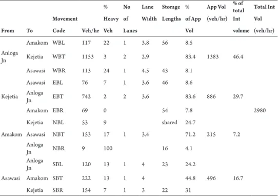
From Table 1, the intersection registered a peak hour volume of 2,980 vehicles. This value
represented the worst traffic situation for an average day. Therefore, the existing control needs to be replaced with a more effective, efficient and reliable control scheme to ensure smooth and safe operations of all types.
2.6.2. Signal Control Data for Amakom
Intersection
Cycle length is the time required for one complete sequence of signal indications (phases). Usually it is measured in seconds. Cycle lengths and phases for the intersection were recorded using stopwatch. Cycle length for intersection was obtained as 172 seconds. Table 2 shows the signal timing data.
Table 1
Summary Peak Hour Traffic Volume and Geometric Data at Amakom Intersection
% No Lane Storage % App Vol % of
total Total Int
Movement Heavy of Width Lengths of App (veh/hr) Int Vol
From To Code Veh/hr Veh Lanes Vol volume (veh/hr)
Amakom WBL 117 22 1 3.8 56 8.5
Anloga
Jn Kejetia WBT 1153 3 2 2.9 83.4 1383 46.4
Asawasi WBR 113 24 1 4.5 43 8.1
Asawasi EBL 76 7 1 3.6 46 8.6
Kejetia Anloga
Jn EBT 742 2 2 3.6 83.6 886 29.7
Amakom EBR 69 0 54 7.8 2980
Kejetia NBL 53 9 shared 24.7
Amakom Asawasi NBT 153 17 1 3.4 71.2 215 7.2
Anloga
Jn NBR 9 100 16 4.1
Anloga
Jn SBL 120 13 1 4 23 24.2
Asawasi Amakom SBT 222 13 1 4 44.8 496 16.7
Table 2
Signal Timing Data at Amakom Intersection
Direction Cycle
Length (C)
Actual Green Time (G)
Actual Yellow Time (Y)
Actual Red Time (R)
Total Lost Time (l1+l2)
Effective Green Time (g)
From KNUST 172 56 4 2 4 58
To KNUST 172 47 4 2 4 49
The resulting effective green time (g) was therefore calculated using the Eq. (4) below:
(4)
Where:
l1 = start up lost time,
l2 = clearance lost time.
2.7. Calibration Data for Amakom
Intersection
In order to realistically model traffic at the intersection, it is important to have realistic calibration data. To calibrate the model for local conditions, speed and headway data were collected.
2.7.1. Spot Speed Data
Speed is the most important parameter describing the state of a given traffic stream. In a moving traffic stream, each vehicle travels at a different speed. Thus, the traffic stream does not have a single characteristic speed but rather a distribution of individual vehicle speeds. The spot speed data to and from KNUST approaches at the intersection were collected using the Doppler principle (radar). The speed data were collected as the tail of the vehicles crosses the stop bar. The first four vehicles in queue were not counted because they were accelerating from rest. A radar gun was operated by a single person. Operators randomly targeted the vehicles
and recorded the digital readings displayed on the unit. Through traffic speeds to and from KNUST approaches at the intersection were recorded for a maximum of 60 vehicles inclusive of private cars, commercial vehicles and heavy goods vehicles.
2.7.2. Headway and Saturation Flow Data
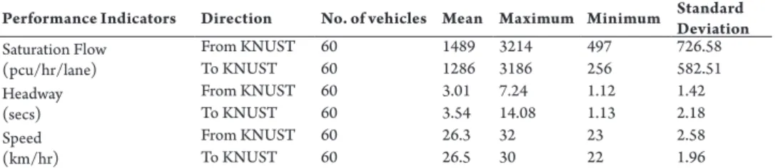
The headway is the time starting from when the tail of the lead vehicle crosses the stop bar until the front of the following car crosses the stop bar. Headway data for three cycles each were collected with a stopwatch at the intersection. Table 3 shows the summary of computed saturation flow, headway and speed for the intersection.
2.8. Calibration of the Synchro Models
2.8.1. Chi Square Test Analysis (p-Values)
This was used to determine the level of significance between the computed and simulated saturation f low, speeds and headways for the intersection. When p < 0.05, it was considered as significant and if p > 0.05 was considered not significant.
2.8.2. Paired Sample T-Test Analysis
2.8.3. Regression Analysis
Calibration of the model was based on regression analysis using traffic volume data to-and-from KNUST approaches of the Amakom intersection. It was carried out to establish whether speed or headway had a strong correlation with saturation flow. The predictors were speed and headway whiles the dependent variable was saturation flow.
2.9. Performance Assessment at
Amakom Intersection
Levels of Service (LOS) and delay were used to assess the performance at the intersection. A Level of service is a letter designation that describes a range of operating conditions on a particular type of facility. The 1994 Highway Capacity Manual defines levels of service as “qualitative measures that characterize operational conditions within a traffic stream and their perception by motorists and passengers.” Six levels of service are defined for capacity analysis. They are given letter designations A through F, with LOS A representing the best range of operating conditions and LOS F the worst. Delay is defined in terms of the average stopped time per vehicle traversing the intersection.
2.9.1. Change of Phase without Geometric
Improvement
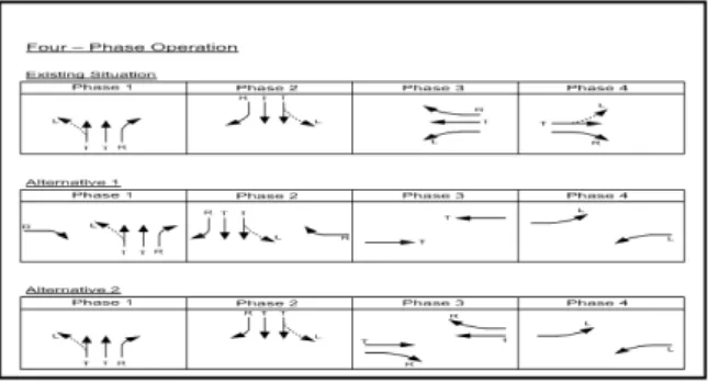
For effective investigation of the optimized
cycle lengths and offsets for A makom signalized intersection on the corridor, two different alternatives with four-phase operational plan in Fig. 3 were proposed.
2.9.2. Change of Phase with Geometric
Improvement
The best alternative chosen was further investigated upon by the addition of lane(s) to the through put traffic at the intersection. This was done to determine improvements in the level of service. This is because improvement in the level of service at the intersection would result in overall and enhanced performance on the road corridor.
2.9.3. Grade Separation Option
Cont i nuous add it ion of la nes to t he through put traffic will adversely affect the reservations at the intersection and when that condition persists, grade separation option will be considered to see how best to allow free flow of traffic to traverse the intersection concerned.
3. Results and Discussion
3.1. Saturation Flow, Headway and Speed
Data
Table 3 shows the summary of computed saturation flow rates, headways and speed for Amakom intersection.
Table 3
Computed Saturation Flow, Headways and Speed Data
Performance Indicators Direction No. of vehicles Mean Maximum Minimum Standard
Deviation Saturation Flow
(pcu/hr/lane)
From KNUST 60 1489 3214 497 726.58
To KNUST 60 1286 3186 256 582.51
Headway (secs)
From KNUST 60 3.01 7.24 1.12 1.42
To KNUST 60 3.54 14.08 1.13 2.18
Speed (km/hr)
From KNUST 60 26.3 32 23 2.58
3.2. Explanation of Saturation Flow
Values
Saturation flow, which is the maximum rate of f low of traffic across the stop line at an intersection, is a very important measure in Junction design and signal control applications. Low values of Saturation f low means less vehicles can cross the stop line when the signal turns green. Data collection techniques for the determination of saturation flow are well elaborated by the Transport Research Laboratory United Kingdom (TRB, 1993).
The saturation flow from KNUST junction approach was 1489 pcu per hour per lane and that to KNUST junction approach was 1254 pcu per hour per lane at the intersection. This was attributed to vehicle mix, geometry of intersection, driver behaviour, public transport proportion in traffic stream, stops near intersection along routes (within 20
m) and pedestrian indiscriminate crossing due to location of attractions and roadside activity. These were identified as principal factors affecting f low, which collaborates Turner and Harahap (1993); Liu et al. (2005) and Minh et al. (2003), who have severally reported similar results. The presence of fuel service stations, high pedestrian volumes and erratic pedestrian crossing and roadside activities significantly affected the saturation flows at the intersection.
3.3. Results of Calibration of Synchro
Models
3.3.1. Chi-Squared Analysis (p-Values)
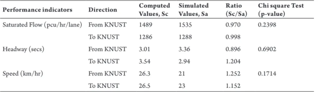
Table 4 shows the results of the comparison between computed and simulated saturation f low, speeds and headways for Amakom intersection using the Chi Square Test (p-value).
Table 4
Comparison of Computed and Simulated Performance Indicators
Performance indicators Direction Computed
Values, Sc
Simulated Values, Sa
Ratio (Sc/Sa)
Chi square Test (p-value) Saturated Flow (pcu/hr/lane) From KNUST 1489 1535 0.970 0.2398
To KNUST 1286 1288 0.998
Headway (secs) From KNUST 3.01 3.36 0.896 0.6902
To KNUST 3.54 2.94 1.204
Speed (km/hr) From KNUST 26.3 21 1.252 0.1714
To KNUST 26.5 23 1.152
P-values > 0.05 meant that there were no significant differences between the computed and simulated values in terms of saturation flow, headway and speed data for the intersection. Indicating that the field saturated flow, headway and speed values were similar to the simulated saturated flow, headway and speed values obtained from Synchro.
3.3.2. T-Test Analysis
that there was no significant (p > 0.05) difference between the computed and simulated headway values.
For speeds however at each approach of the intersection, the test results showed that there was significant (p < 0.05) difference bet ween the computed and simulated
speed values. It was found that a certain percentage of the variation in the simulated speed values was explained by the field speed values and Eta squared values explained in Table 5 that provide detailed results of level of significance test carried out at Amakom Intersection (t-test analysis).
Table 5
Results of Paired Sample Test at Amakom Intersection (Sat Flow SIM)
Approaches
Paired Difference
t
Eta squared (%)
Sig. (2-tailed) p-value
Mean Standard
deviation
Standard error mean
95% confidence interval of the difference
Lower Upper
Saturation from
KNUST -45.800 728.645 94.068 -234.029 142.429 -0.487 0.4 0.628
Saturation to
KNUST -2.683 580.118 74.893 -152.54 147.177 -0.036 0.0022 0.972
Speed from KNUST 5.300 1.843 0.291 4.711 5.889 18.193 84.9 0.000
Speed to KNUST 3.475 1.198 0.189 3.092 3.858 18.345 85.1 0.000
Headway from
KNUST -0.353 1.414 0.183 -0.719 0.119 -1.936 6.0 0.058
Headway to KNUST 0.600 2.211 0.285 0.029 1.171 2.103 7.0 0.040
Paired t-test results in Table 5 showed there was no significant (p > 0.05)saturation flow variation of vehicular movements between the field and the simulated situation for approaches from both direction. Eta squared statistic 0.004 indicated a small size effect; meaning only 0.4% of the variation in the simulated saturation f low was explained by the field saturation flow from KNUST. Again Eta squared statistic 0.000022 indicated a small size effect which meant that only 0.0022% of the variation in the simulated saturation f lows was explained by the field saturation to KNUST. There was significant (p < 0.05)speed variation of vehicular movements between the field and the simulated situation for approaches from both direction. Eta squared statistic 0.849 indicated a large size effect; meaning 84.9% of the variation in the simulated
3.3.3. Regression Analysis
From the analysis, it was established that headway had a strong correlation with
saturation f low from KNUST approach with R2
field = 0.748 and R 2
simulated = 1.000. Similarly, headway had a strong correlation with saturation flow to KNUST approach with R2
field = 0.683 and R 2
simulated = 1.000.
Table 6
Comparison of Field and Simulated Saturation Flow, Speed and Headway
From KNUST Approach R R Square (R2) Adjusted R Square
(R2)
Standard Error of the Estimate
Field Conditions 0.865 0.748 0.735 367.072
Simulated Conditions 1.000 1.000 1.000 0.000
The adjusted R2 value was expressed in percentage as 73.5%. Thus the model (headway and speed) explained 73.5% of the variance in the saturation flows for field condition as shown in Table 6. Similarly,
the adjusted R2 value was expressed in percentage as 100%. Thus the model (headway and speed) explained 100% of the variance in the saturation f lows for simulated condition.
Table 7
Results of Field and Simulated Conditions Co-Efficients
Predictors
Unstandardized Coefficients
Standardized
Coefficients t Sig.
Collinearity Statistics
B Std. Error Beta Tolerance VIF
Constant 2714.454 622.587 4.360 0.000
Speed from KNUST
Approach 6.586 22.765 0.024 0.289 0.774 0.998 1.002
Headway from
KNUST Approach -476.444 45.546 -0.864 -10.461 0.000 0.998 1.002
Constant 1199.000 0.000 5x10⁸ 0.000
SpeedSIM 1.27x10⁻¹⁴ 0.000 0.000 0.000 1.000 0.877 1.141
HeadwaySIM 100.000 0.000 1.000 3x10⁸ 0.000 0.877 1.141
For the field condition, the model established that headway (- 0.864) made a unique contribution in explaining the saturation f low when the variance in the model was controlled for as compared to that of speed (0.024) which made a less contribution to the model as can be seen in Table 7. Headway has a significance level of 0.000 which was less than 0.05; thus greatly contributed to the prediction of saturation flow whiles speed (0.774) made insignificant contribution.
The field equation connecting saturation flow (q), speed (u) and headway (h) is (Eq. (5)):
(5)
of speed (0.000) which made no contribution to the model as can be seen in Table 7. Headway has a significance level of 0.000 which made significant contribution to the prediction of saturation flow whiles speed (1.000) made an insignificant contribution.
T he si mu lated equ at ion con nec t i ng saturation flow (q), speed (u) and headway (h) is (Eq. (6)):
(6)
Table 8
Comparison of Field and Simulated Saturation Flow, Speed and Headway
To KNUST Approach R R Square (R2) Adjusted R Square (R2) Standard Error of the
Estimate
Field Conditions 0.827 0.685 0.668 337.738
Simulated Conditions 1.000 1.000 1.000 0.232
The adjusted R2 value was expressed in percentage as 66.8%. Thus the model (headway and speed) explained 66.8% of the variance in the saturation flows for field condition. Similarly, the adjusted R2 value
was expressed in percentage as 100%. Thus the model (headway and speed) explained 100% of the variance in the saturation flows for simulated condition as can be seen in Table 8.
Table 9
Results of Field and Simulated Conditions Co-Efficients
Predictors
Unstandardized Coefficients
Standardized
Coefficients t Sig. Collinearity Statistics
B Std. Error Beta Tolerance VIF
Constant 3073.799 1014.829 3.029 0.004
Speed to KNUST
Approach -24.841 34.732 -0.083 -0.715 0.479 0.630 1.586
Headway to KNUST
Approach -333.976 44.364 -0.875 -7.528 0.000 0.630 1.586
Constant 983.996 1.376 715.028 0.000
Speed SIM 0.270 0.045 0.012 5.969 0.000 0.877 1.141
Headway SIM 101.318 0.203 1.004 499.941 0.000 0.877 1.141
For the field condition, the model established that headway (-0.875) made the strongest contribution in explaining the saturation f low when the variance in the model was controlled for as compared to that of speed (0.083) which made a less contribution to the model as shown in Table 9. Headway had a significance level of 0.000 which was less than 0.05; thus greatly contributed to the prediction of saturation flow whiles speed (0.479) made an insignificant contribution.
The field equation connecting saturation flow (q), speed (u) and headway (h) is (Eq. (7)):
(7)
speed (0.012) which made a less contribution to the model as shown in Table 9. Headway had a significance level of 0.000 which was less than 0.05; thus greatly contributed to the prediction of saturation flow as well as speed (0.000).
T he si mu lated equ at ion con nec t i ng saturation flow (q), speed (u) and headway (h) is (Eq. (8)):
(8)
3.4. Comparison of Computed and
Simulated Performance Indicators
Computed manual performance indicators at the intersection were compared with the simulated performance indicators generated by the calibrated Synchro model as shown in Table 10 below.
Table 10
Comparison of Computed and Simulated Performance Indicators
Performance Indicators
Amakom
Computed Simulated
Cycle Length (sec) 172 193
Volume to capacity ratio (v/c) ratio 1.78 1.48
Intersection Delay (sec) 126 157.1
Intersection Level of Service, LOS F F
Intersection Capacity Utilization, ICU (%) 67.6
Offsets 133
The level of service F described a forced-flow operation at low speeds, where volumes were below capacity. These conditions usually resulted from queues of vehicles backing up a restr iction dow nstream. Speeds were reduced substantially and stoppages occurred for short or long periods of time because of the downstream congestion. It represented worst conditions.
3.5. Analysis of Alternative Phasing Plans
3.5.1. Change in Phasing Plan without
Geometric Improvement
Fig. 3 below shows the existing traffic situations together with their possible alternative phasing plans at the Amakom intersection.
Fig. 3.
Table 11
Results of Performance Indicators for Two Different Alternatives
Performance Indicators Existing Situation Alternative 1 Alternative 2
Cycle Length 193 170 172
v/c ratio 1.48 1.48 1.48
Int. Delay (s) 157.9 154.6 160.3
Int. LOS F F F
ICU (%) 67.6 67.6 67.6
Offsets 133 133 133
Out of the two possible alternative phasing plans at the Amakom intersection, alternative 1 gave out the best optimized cycle length of 170 secs with an offset of 133 secs and an intersection delay of 154.6 secs as shown in Table 11. These indicators compared to the existing indicators were better in terms of cycle length, v/c ratio and delay. Level of service F described a forced-flow operation at low speeds, where volumes were below capacity. These conditions usually resulted from queues of vehicles backing
up a restr iction dow nstream. Speeds were reduced substantially and stoppages occurred for short or long periods of time because of the downstream congestion. It represented worst conditions.
3.5.2. Change in Phasing Plan with
Geometric Improvement
The best alternative in Fig. 3 was further investigated upon by adding lane(s) to the through put traffic at Amakom intersection.
Table 12
Performance Indicators with Geometric Improvement
Performance Indicators
Existing Situation Alternative 1 Addition of 1 lane Addition of 2 lanes
Cycle Length 193 170 170 170
v/c ratio 1.48 1.48 1.03 0.82
Int. Delay (s) 157.9 154.6 73.9 60.4
Int. LOS F F E E
ICU (%) 67.6 67.6 49.8 43.6
Offsets 133 133 133 133
Geometric improvements were done as a correctional measure. With the addition of one lane on the major approach through put traffic, the v/c ratio reduced from 1.48 to 1.03 with a corresponding reduction in delay as seen in Table 12. The level of service also changed from F to E meaning that there had been an improvement at the intersection. When 2 lanes each were added to each major through put approach, the v/c ratio again reduced from
It represented intermediate conditions and performance had improved slightly at the intersection. Similarly, the existing reservation was further checked against the geometric improvement.
3.6. Grade Separation Option
With the continuous addition of lanes to the through put traffic on the major approaches at Amakom intersection, a situation may arise where there will not be enough space to contain the addition of lanes. Since the intersection will still be operating at a level of service E, there is therefore the need to provide a facility that can accommodate the traffic congestion at the intersection on a long term basis. This then calls for a grade separation (interchange) at the intersection to allow the free and continuous movement of vehicles thereby minimizing congestion.
4. Conclusion
It was concluded at 5% significant level, the Chi square test and t-test analyses revealed that headway had a strong correlation with saturation flow for both field and simulated conditions. Again changes in phasing plan without geometric improvement at the intersection did not improve upon the overall intersection’s level of service. Furthermore changes in phasing plan with geometric improvement enhanced the intersection’s level of service. The existing control needed to be replaced with a more effective, efficient and reliable control scheme to ensure smooth and safe operations. An interchange therefore should be constructed at the A makom intersection to allow free movement of vehicles thereby minimizing congestion and accident occurrences.
Acknowledgements
The authors would like to acknowledge the management of Kumasi Polytechnic, Kumasi headed by the Rector Prof. N.N.N. Nsowah-Nuamah, for providing financial assistance and also Department of Urban Roads (DUR), Kumasi for giving information on signalized intersections in the Kumasi Metropolis. Several supports from staff of the Civil Engineering Department, KNUST and Kumasi Polytechnic, Kumasi are well appreciated.
References
BCEOM and ACON Report. 2004. Consultancy Services for Urban Transport Planning and Traffic Management Studies for Kumasi and Tamale for DUR, Ministry of Transportation, Ghana. Chapter 5, 37-52.
Brackstone, M.; McDonald, M. 1999. Car-following: a historical review, Transportation Research Part F: Traffic Psychology and Behaviour. DOI: http://dx.doi.org/10.1016/ S1369-8478(00)00005-X, 2(4): 181-196.
Drew, D.R. 1968. Traffic flow theory and control. New York: McGraw-Hill.
Gazis, D.C.; Herman, R.; Rothery, R.W. 1961. Follow-the leader models of traffic flow, Operations Research. DOI: http://dx.doi.org/10.1287/opre.9.4.545, 9(4): 545-567.
Gerlough, D.; Huber, M. 1975. Traffic flow theory. A monograph. TRB Special Report 165. Washington, D.C.
Gunay, B. 2007. Car following theory with lateral discomfort, Transportation Research Part B: Methodological. DOI: http://dx.doi.org/10.1016/j.trb.2007.02.002, 41(7): 722-735.
Jin, S.; Wang, D.H.; Tao, P.F.; Li, P.F. 2010. Non-lane-based full velocity difference car following model. Physica A:Statistical Mechanics and its Applications. DOI: http:// dx.doi.org/10.1016/j.physa.2010.06.014, 389(21): 4654-4662.
Kallberg, H. 1971. Traffic simulation (in Finnish). Licentiate Thesis, Helsinki University of Technology, Transportation Engineering. Espoo.
Kikuchi, C.; Chakroborty, P. 1992. Car following model based on a fuzzy inference system. Transportation Research Record, 1365: 82-91.
Liu, P.; Lu, J.J.; Fan, J.; Pernia, J.C.; Sokolow, G. 2005. Effect of U-Turns on Capacity of Signalized Intersections, Transportation Research Record, Journal of the Transportation Research Board. DOI: http://dx.doi. org/10.3141/1920-092005, 1920(2005): 74-80.
Luo, L.H.; Liu, H.; Li, P.; Wang, H. 2010. Model predictive control for adaptive cruise control with multi-objectives: comfort, fuel-economy, safety and car-following, Journalof Zhejiang University-SCIENCE A (Applied Physics andEngineering). DOI: http://dx.doi. org/10.1631/jzus.A0900 374, 11(3): 191-201.
Mathew, T.V.; Radhakrishnan, P. 2010. Calibration of micro simulation models for nonlane-based heterogeneous traffic at signalized intersections, Journal of UrbanPlanning and Development. DOI: http://dx.doi. org/10.1061/(ASCE)0733-9488(2010)136:1(59), 136(1): 59-66.
McDonald, M.; Brackstone, M.; Sultan, B. 1998. Instrumented vehicle studies of traffic flow models. In Proceedings of the Third International Symposium on Highway Capacity, Copenhagen, Denmark. 755-773.
Minh, C.C.; Sano, K.; Tanaboriboon, Y. 2003. Traffic Policy Evaluations Using Micro Traffic Simulation: A Case Study of Thailand, Paper for Presentation at the 2003 Meeting of the Transportation Research Board, Washington, D.C., USA.
Newell, G.F. 1961. Nonlinear effects in the dynamics of car following, Operations Research. DOI: http://dx.doi. org/10.1287/opre.9.2.209, 9(2): 209-229.
Tordeux, A.; Lassarre, S.; Roussignol, M. 2010. An adaptive time gap car following model, Transportation ResearchPart B: Methodological. DOI: http://dx.doi. org/10.1016/j.trb.2009.12.018, 44(8-9): 1115-1131.
Transportation Research Board. 1993. Highway Capacity Manual, Chapter 9 (Signalized Intersections), National Research Council, Washington, D.C.
Turley, C. 2007. Calibration Procedure for a Microscopic Traffic Simulation Model. A Thesis submitted to the Faculty of Brigham Young University, 2-19.
Turner, J.; Harahap, G. 1993. Simplified Saturation Flow Data Collection Method: Overseas Centre, Transport Research Laboratory, Crowthorne Berkshire RG456AU, United Kingdom, PA1292/93.
W ie de m a n n , R . 19 74 . S i mu l at ion de s St r a ß Enverkehrsf lusses Schriftenreihe des Instituts für Verkehrswesen der Universität Karlsruhe (in German).