www.ann-geophys.net/26/2037/2008/ © European Geosciences Union 2008
Annales
Geophysicae
Three-dimensional spectrum of temperature fluctuations in stably
stratified atmosphere
A. S. Gurvich and I. P. Chunchuzov
Oboukhov Institute of Atmospheric Physics, Moscow 119017, Russia
Received: 27 February 2008 – Revised: 24 April 2008 – Accepted: 16 June 2008 – Published: 28 July 2008
Abstract.A phenomenological model is proposed for a 3-D spectrum of temperature inhomogeneities generated by inter-nal waves in the atmosphere. This model is a development of the theory based on the assumption that a field of Lagrangian displacements of fluid particles, induced by an ensemble of internal waves with randomly independent amplitudes and phases, is statistically stationary, homogeneous, axially sym-metric in horizontal plane and Gaussian. For consistency of this model with measured spectra of temperature fluctuations in the stratosphere and mesosphere the additional assump-tion was introduced in to the model about the anisotropy of inhomogeneities to be dependent on their vertical sizes. The analytic expressions for both the 3-D and 1-D spectra are obtained. A model vertical wave number spectrum fol-lows a−3 power law, whereas a horizontal spectrum con-tains two regions with a−3 slope, and the intermediate re-gion with the slope between−1 and −3 depending on the rate of anisotropy decrease as a function of increasing sizes of the inhomogeneities. In the range of a few decades the model showed a good agreement with the results of mea-surements of the spectra in the troposphere, stratosphere and mesosphere.
Keywords. Meteorology and atmospheric dynamics (Mid-dle atmosphere dynamics; Turbulence; Waves and tides)
1 Introduction
In this paper we propose a model of three-dimensional (3-D) spectrum of the temperature fluctuations in stably strati-fied atmosphere with the vertical scales ranging from a few meters to several kilometers. Such scales are typical for at-mospheric internal gravity waves (IGWs), which is known to form 3-D anisotropic temperature irregularities.
Correspondence to:I. P. Chunchuzov ([email protected])
When trying to parameterize the influence of IGWs on general atmospheric circulation we need a model of 3-D spectrum of IGWs in the atmosphere, since the parameter-ization models of wave drag are sensitive to the height de-pendence of this spectrum and to the vertical scale of wave breaking processes (Fritts and Alexander, 2003; McLan-dress, 1997; Hynes, 2005). The 3-D spectrum also deter-mines the statistical properties of electromagnetic and acous-tic waves propagating through the atmosphere (Tatarskii, 1971). The physical mechanisms explaining the observed forms of 1-D vertical and horizontal spectra of wind and temperature fluctuations were explored in a number of pa-pers (VanZandt, 1982; Sidi et al., 1988; Dewan, 1997; Lind-borg, 2006). However, the question about the form of a 3-D spectrum of these fluctuations, which produces such 1-3-D spectra, remained open. It was shown in Chunchuzov (2002) (hereafter Ch02) that strongly anisotropic 3-D temperature and wind speed irregularities can occur in non-linear field of random internal waves in stably stratified atmosphere. Equi-librium 3-D spectrum obtained in this study results from the balance between the nonlinear wave energy transfer from wave sources with some characteristic vertical and horizon-tal scales towards lesser vertical scales (and simultaneously towards larger horizontal scales), and dissipation of the wave energy due to the wave breaking at certain scale. However, the Ch02 theory did not take into account a reverse influence of the turbulence, generated by breaking waves, on the wave spectrum itself. The emerging turbulent diffusion results in smoothing of the spatial gradients of the wave field, and af-fects characteristic vertical and horizontal scales of the field variations, and therefore its anisotropy.
2 The theory
An approximate expression for regularized 3-D spectrum of temperature fluctuations may be derived from the 3-D spec-trum of vertical displacements induced by a random internal wave field (Ch02):
8(T0)(κ)=
A0T02ωBV4
g2|κ
z|5
exp − κ
2
⊥
4e0κz2
! R
|κz|
κ∗ , b
,
κ⊥2 =κx2+κy2, e0≪1, (1)
where ωBV is Brunt-V¨ais¨al¨a (BV) frequency, T0 –
unper-turbed temperature at a given altitude,g– gravity accelera-tion,e0is a coefficient proportional to the variance of the
hor-izontal gradient of a random Lagrangian field of the air parti-cle’s vertical displacements, andA0=β0/(8π e0)is a
nondi-mensional coefficient withβ0=0.1÷0.3.
The function8 (κ)is considered to be a spectrum of lo-cally homogeneous random field under the condition of ex-istence of the corresponding structure function. The Eq. (1) results from Eq. (55a) in Ch02 after myltiplying Eq. (55a) by a factorR, which provides a regularization of the spectrum over the region of small wavenumbers|κ| →0 for|κz|<κ
∗;
κ∗is a characteristic vertical wave number of the spectrum. The introduced regularization factor R (ζ, b)≤1 possesses the following properties: the ratio R (ζ, b)ζb is finite at ζ→0 andR (ζ, b)→1 for ζ >1; b>0 is the regularization parameter.
Calculation from Eq. (1) of the one-side vertical wavenumber spectrum results in
VT(0,v)(κz)=2
Z Z
8(T0)(κ) dκydκx
=β0
T02ω4BV g2κ3
z
R κ
z
κ∗, b
, κz>0, (2)
Forβ0=0.1÷0.3 Eq. (2) is consistent with numerous
exper-imental data reviewed by Fritts and Alexander (2003) (here-after FA03). Also, calculation of the horizontal spectrum VT(0,h) κy=RR8T (κ) dκydκz leads to the −3 power law decay, VT(0,h) κy∼
κy
−
3
, for κy
>κ∗
√
2e0. Once the
scalingκy′=κy√2e0is applied, a one-side horizontal
spec-trumV(0,h)coincides withV(0,v)κy′atκy′>κ∗. The less is the value of√2e0, the more 3-D spectrum is stretched along
Oκz-axis and, accordingly, the irregularities are more
flat-tened in vertical direction. This suggests that 1.√2eis a measure of anisotropy of the irregularities. Since the parame-tere0is considered as constant (Ch02), Eq. (1) can be looked
upon as a model of 3-D spectrum with constant anisotropy. Measured horizontal spectra (Vinnichenko et al., 1980, Nastrom and Gage, 1985; Hostetler at al., 1991; Bacmeis-ter et al., 1996; Cho et al., 1999; Lindborg, 1999) re-veal the existence of spectral intervals where the depen-dence V(0,h) κy
differs from κy
−
3
. In order to fit
the model of the vertical and horizontal spectra, deter-mined by 3-D spectrum, to the measurements, we modify Eq. (1), taking into account a possibility for the anisotropy of temperature irregularities to vary with their vertical sizes. We illustrate the concept of variable anisotropy η by us-ing the structure function DT (δr)=DT(δr
⊥, δz) where
δr2
⊥=δx
2
+δy2. We assume thatηdepends on vertical sizes of irregularities being a solution of the following equation: DT(0, δz)=DT (η (δz) δz,0). In other words the anisotropy
depends on vertical sizes of irregularities, or using spectral language: η=η (κz). It was shown by Gurvich (1997) that
axis-symmetric 3-D spectrum with a varying anisotropy may produce the 1-D vertical and horizontal power spectra with different power indexes. Introducing a variable anisotropy into the model of 3-D spectrum, we should conserve the de-pendence |κz|−3 for the vertical spectrum regardless of the
form ofη=η (κz). Under our assumptions, the equation for
3-D temperature spectrum with variable anisotropy can be written as follows:
8T(κ)= 1 2
AT02ωBV4 η (κz)2
g2|κz|5 exp −
κ⊥2η (κz)2 2κ2 z ! R |κz| κ∗ , b
,
κ⊥2 =κx2+κy2, η (κz)≥1, (3) whereAis a numeric multiplier to be found from comparison (3) with the experimental data. Forη=const case, Eq. (3) is consistent with Eq. (1), taking into account the notation differences. The model (3) allows us to calculate the 1-D spectraVT (κs;α)for the arbitrary direction having an angle
ofαwith respect to the horizontal plane
VT (κs;α)=
Z ∞
−∞
dκxdκydκz8T κx, κy, κz
δ κycosα+κzsinα−κs (4)
whereδ (ζ ) is Dirac’s delta function. The anglesα=π 2 andα=0 correspond to the horizontal and vertical spectra, respectively. The Eq. (4) is a compact expression for the in-tegration along the plane, which is at a distanceκs from the
coordinate origin and has the angle ofπ2−αwith respect to the planeκxOκy.
To compare model (3) with the measurements, let us calcu-late vertical and horizontal spectra. The result of integration of Eq. (3) overdκxdκyshows that vertical spectrumVT(v)(κz)
does not depend onη (κz)and is similar to Eq. (2) at|κz|>κ∗
after replacingβ0by the numeric coefficientβ=2π A. The
dependence ofVT(v)(κz)on the regularizing factor R is
es-sential only at|κz|<κ∗.
Horizontal spectra calculation for model (3) results in the following equation
VT(h) κy=β
√ 2πT
2 0ωBV4
g2κ3
y
∞
Z
0
dςη κyς ς−4 R
κy
κ∗ ς, b
exp −
1 2
η κyς
ς !2
, κy>0. (5)
To compare Eq. (5) with the measurements, it is neces-sary to specify the functionsR (ζ, b) andη (κz). We will
use the easiest version: R (ξ;b)=ξb ξb+1. Function η (κz) will be chosen by using the available results of the
measurements in the upper troposphere and lower strato-sphere. The measurements conducted in Nastrom and Gage (1985) (hereafter NG85), show that VT(h) κy∼
κy − 3 for 2×10⁻⁶<
κy
<6×10⁻⁵ rad/m. This suggests that η (κz)
has a constant value of the order of many tens, or hundreds, for wavenumbersκ∗<κz<κM corresponding to the
largest-scale irregularities with the vertical sizes of about one kilo-meter or more. Measured angular dependence of the scatter-ing cross-section of MST radar radiation (Doviac and Zrnic, 1984; Gurvich and Kon, 1993; Hermawan et al 1998) indi-cates that noticeable anisotropyη0>1 still exists for
small-scale stratospheric irregularities with vertical sizes of the or-der of a few meters. The analysis of star scintillation spec-tra observed from satellite through the Earth’s sspec-tratosphere (Gurvich and Kan, 2003; Gurvich and Chunchuzov, 2003) leads to the same conclusion. To defineη (κz)for
intermedi-ate scales, we suggest the following interpolintermedi-ated formula
η κ
z
κw
=η0
1+ κ w κM p
, if |κz|< κM;
η κ
z
κw
=η0
1+ κw κz p
, if |κz|> κM;p >0 (6)
which will be tested using the complex of measurements. The parameterpin Eq. (6) determines the rate at which the anisotropy decreases with decreasing vertical sizes of irreg-ularities. As to the irregularities with the vertical sizes less than 1
κw, their anisotropy is small (η=const) and do not
substantially change in the process of their evolution. Calcu-lation of Eq. (5) using Eq. (6) results in the following asymp-totic equations:
VT(h) κy∼β
T02ωBV4 g2 η−
2
Mκ−
3
y , κ∗ηM ≪κy≪κMηM (7)
VT(h) κy
∼βT
2 0ω4BV
g2
2 3+p
2+2p√2π
π (3+p)Ŵ
5+3p 2+2p
κ− 3+p p+1
y
η 2
p+1 0 κ
2p p+1
w
, κM
ηM ≪κy≪κw
η0 (8)
VT(h) κy∼β
T02ωBV4 g2 η−
2 0 κ−
3
y , κy> κwη0. (9)
The wider the interval of acceptable values ofκy, the better
approximation is provided by Eqs. (7–9). These equations
κ
κ
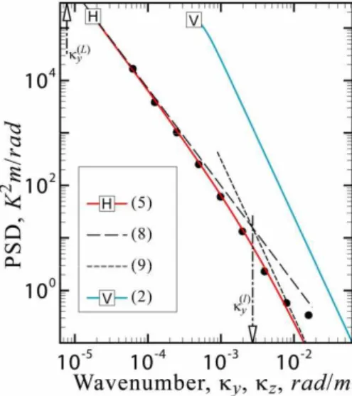
Fig. 1.Comparison of the modeled horizontal (H) and vertical (V) spectra with the measurements (Nastrom and Gage, 1985). The dots depict the measurements. The equations used to calculate spec-tral densities (solid curves) and the asymptotic power-law functions (dashed straight lines), are referred to in the legend. Vertical arrows indicate the abscissas for the intersection points of the curves (7) with (8) (labeled byκy(L)), and (8) with (9) (labeled byκy(l)).
simplify the analysis of Eq. (5) and demonstrate that the hor-izontal spectrum may consist of the three consecutive inter-vals, two of which have a power of−3, while the power for the intermediate range (8) is−(3+p)(p+1). The latter can take the values from−3 to−1.
3 Comparison with measurements
The validation of Eqs. (3) and (5) was made using mea-sured 1-D horizontal spectra (NG85; Hostetler at al., 1991; Bacmeister et al., 1996). The data presented in NG85 were gathered during several thousands of flights and were strongly verified by the measurements (Cho et al., 1999; Lindborg, 1999). The dots in Fig. 1 show the estimated values of the horizontal spectrum from NG85. The latter, unfortunately, does not provide all the characteristics of the measurement conditions. Thus, additional considerations are required to choose the missing parameters of the model spec-tra, which are necessary for calculations. The values of g=9.81 m/s2andT0=220 K are beyond questioning. It
fol-lows from Eqs. (7–9) that the behavior of 1-D horizontal spectrum at wavenumbersκy>κ∗ηM is not very sensitive
to the regularization parameterb, therefore the value ofb=5 has been chosen. The BV frequencyωBVwas assumed to be
ωBV=0.02 rad/s. The valueκy≈10−6 corresponding to the
range, where spectral density measured by NG85 becomes saturated, represents the estimate of the initial characteristic horizontal wavenumberκ∗
ηM. The valueκy=10−5rad/m,
corresponding to the inflection interval of the measured spec-trum, became the basis for the initial estimate ofκM. The
Fig. 2.Comparison of the modeled horizontal (H) and vertical (V) spectra with the measurements (Bacmeister et al., 1996). The dots depict the measurements. The equations used to calculate spectral densities (solid curved lines) and the asymptotic power-law func-tions (dashed straight lines), are referred to in the legend. Vertical arrows indicate the characteristic wavenumbers.
possible value ofη0 is about ten. Final adjustment of the
parameters in Eqs. (5) and (6) was made using a trial-and-error method. Characteristic wavenumbers were found to be κ∗=4.47×10⁻⁴,κ
M=1.5×10⁻³,κw=10−2rad/m. The
val-uesp=2 andη0=9 was found to provide the best fit to the
measured spectra. The obtained valueβ=0.22 is in a good agreement with the numerous measurements of the vertical spectra (FA03), therewith the valueηM=409 is derived.
Fig-ure 1 shows the model spectrumVT(h) κy, calculated from
Eq. (5), which depicts all the details of the NG85 measure-ments. The vertical spectra are not presented by NG85 , but the model (3) allows one to obtain them, given the parameters calculated from the measurements of horizontal spectrum. The vertical spectrum VT(v)(κz), calculated accordingly to
Eq. (2), is also shown in Fig. 1. Relations (7–8) depict in Fig. 1 the two power-law intervals of the measured spectrum with power indexes−3 and−5/3. Note that the model is in good agreement with the measurements throughout the wavenumber range of more than three decades. Theky−3 -shape of the low-wavenumber part of the NG85 horizontal spectrum may be interpreted by a theory of quasi-geostrophic turbulence with an enstrophy cascade from longer to shorter horizontal wavelengths (see, for instance, Charney, 1971; Lindborg, 1999, 2006). At the same time, our model suggests that internal wave-wave interactions may also contribute to the same large-scale part of the spectrum (given by Eq. 7) by nonlinear wave energy transfer from shorter horizontal scales. As to the third power-law range (Eq. 9) with the power index of−3, the spatial resolution in the NG85 mea-surements appears to be not good enough to investigate the spectrum at such short scales.
The dots in Fig. 2 depict the measurements of the spec-tra (Bacmeister, 1996), conducted at the altitude of about 20 km. Wavenumber range is expanded by almost one or-der towards large wavenumbers, compared to the NG85 data. However, this range is limited from below by the valueκy
≈6×10⁻⁵rad/m, and this complicates the process of choosing the values ofκ∗ andκM, since they appear to
be below the limiting value of κy
. It follows from the Eqs. (7–9) that the behavior ofVT(h) κyatκy>κMηM has
to depend only slightly onκ∗ andκM. So, to conduct the
comparison, we have taken the same values for these pa-rameters as those used above. The valueωBV=0.022 rad/s
was taken accordingly to the data obtained in Bacmeister (1996, Fig. 11). With previously chosenT0=217 K, η0=9
andβ=0.22, we had to define the parameter p, wavenum-berκw, andβ. The trial-and-error method gave the values:
p=1.35 andκw=9.5×10⁻³rad/m. Given these parameters,
ηM=263 and(3+p)(p+1)=1.85. The last is close to the
value of −1.67 obtained by NG85. The measurements in Bacmeister (1996) fall into the range of transition from the asymptotic dependence to the power-law dependence∼κy−3. The agreement between the model and measurements is quite satisfactory up to κy=8×10⁻³rad/m, above which the
ef-fects of buoyancy forces on spectral power law decay was suggested to become negligibly small (Bacmeister, 1996).
The results of synchronized aircraft-based measurements of vertical and horizontal spectra in the layer between 80 and 105 km were published in Hostetler et al. (1991). The spectra obtained from these measurements and the calculated model spectra, which take into account the effects of averag-ing over the time duration of laser pulse and the time inter-val of the accumulation of scattered photons, are shown in Fig. 3. Using Eq. (2), we obtained an estimateβ=0.28 from the measured vertical spectrum, for which we have chosen the parametersg=9.5 m/s2,T0=160 K andωBV=0.025 rad/s
so as to match the atmosphere model CIRA-61. We point out that the deviation of the model spectrum from power-law dependence∼κz−3 at largeκz results from the time
averag-ing, accounted for in calculations. The remaining parameters were adjusted, as previously, using trial-and-error method. This procedure was complicated by the fact that the range of wavenumbers for the published results of the horizontal spec-tra measurements does not embrace all possible characteris-tic wavenumbers. The best agreement between the model and measurements has been gained for the following param-eters:κ∗=κM=3.9×10⁻⁴rad/m,b=3.5,η0=15, andp=0.6.
For these parameters, the maximum value of the anisotropy coefficientηM=135. Let us dwell on the parameterpwhich
leads to the power index −(3+p)
(1+p)=−2.25. This value is sufficiently close to the estimates for horizontal spec-trum presented in Hostetetler et al. (1994).
Fig. 3.Comparison of the model with the measurements (Hostetler et al., 1991). Vertical (V) and horizontal (H) spectra of the relative density fluctuations are shown. Black solid line: measurements; Mod: model; the equations used to calculate asymptotic power-law functions are referred to in brackets.
(
α
=)
(
α
=)
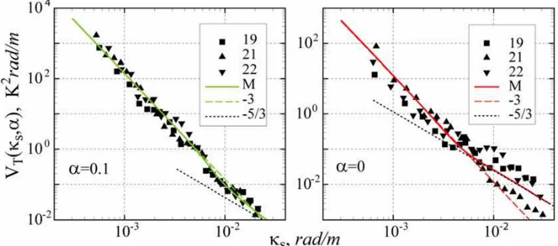
Fig. 4.Comparison of the model with the measurements of Gurvich and Kukharez (2008). Left panel is oblique spectra(α=0.1), right panel is horizontal(α=0)spectra. M is model calculated by using Eq. (4), dot and dash lines is asymptotic power law, symbols are experimental estimations, 19–22 are flight days.
performed in 1988 on 19, 21, and 22 July. The three pairs of the flights were performed through stable stratified layer of the troposphere between altitudes 2.5 and 7.5 km. The measurements of the mean vertical gradient of temperature allowed us to estimate the values ofωBV, which were close
to 0.01 rad/s. The plots of Fig. 4 show the measured oblique and horizontal spectra. Also shown in the plots are the model spectra, which were calculated under mean flight conditions, with the mean temperatureT0=268 K. We used the Eq. (4)
for calculating of the model spectra., for which the best fit-ting parameters were:κM=4.8×10⁻²,κw=1.7×10⁻¹rad/m,
η0=1.6, β=0.25,p=2.For these parameters the maximum
value of the anisotropyηM=22. The plots of Fig. 4 show the
agreement between measured and model spectra, especially for the case of oblique spectrum.
4 Summary
Acknowledgements. This work was supported by RFBR grants: 06-05-64354, 07-05-91555 and 06-05-64229.
Topical Editor U.-P. Hoppe thanks two anonymous referees for their help in evaluating this paper.
References
Bacmeister, J. T., Eckermann, S. D., Newman, P. A., Lait, L., Chan, K. R., Loewinstein, M., Proffit, M. H., and Gary, B. L.: Strato-spheric horizontal wavenumber spectra of winds, potential tem-perature, and atmospheric tracers observed by high-altitude air-craft, J. Geophys. Res., 101(D5), 9441–9470, 1996.
Charney, J. G.: Geostrophic turbulence, J. Atmos. Sci., 28, 1087– 1095, 1971.
Cho, J. Y. N., Chu, Y., Newel, R. E., Anderson, B. E., Barrick, J. D., Gregory, G. L., Sachse, G. W., Carroll, M. A., and Albercook, G. M.: Horizontal wavenumber spectra of winds, temperature, and trace gases during the Pacific Exploratory Missions: 1. Climatol-ogy, J. Geophys. Res., 104(D5), 5697–5716, 1999.
Chunchuzov, I. P.: On the high-wavenumber form of the Eulerian internal wave spectrum in the atmosphere, J. Atmos. Sci., 59, 1753–1772, 2002.
Dewan, E. M.: Saturated Cascade Similitude Theory of Gravity Wave Spectra, J. Geophys. Res., 102, 29 799–29 817, 1997. Doviac, R. J. and Zrnic, D. S.: Reflection and scatter formulas for
anisotropic air, Radio Sci., 19, 325–336, 1984.
Fritts, D. C. and Alexander, M. J.: Gravity Wave Dynamics and Effects in the Middle Atmosphere, Rev. Geophys., 41(1), 1003, doi:10.1029/2001RG000106, 2003.
Gurvich, A. S.: A heuristic model of three-dimensional spectra of temperature irregularities in the stably stratified atmosphere, Ann. Geophys., 15, 856–869, 1997,
http://www.ann-geophys.net/15/856/1997/.
Gurvich, A. S. and Chunchuzov, I. P.: Parameters of the fine den-sity structure in the stratosphere obtained from spacecraft obser-vations of stellar scintillations, J. Geophys. Res., 108(D5), 4166, doi:10.1029/2002JD002281, 2003.
Gurvich, A. S. and Kan, V.: Structure of Air Density Irregularities in the Stratosphere from Spacecraft Observations of Stellar Scin-tillation: 2. Characteristic Scales, Structure Characteristics, and Kinetic Energy Dissipation, Izvestiya, Atmos. Oceanic Phys., 39, 311–321, 2003.
Gurvich, A. S. and Kon, A. I.: Aspect sensitivity of radar returns from anisotropic turbulent irregularities, J. Electromagn. Waves Appl., 7, 1343–1353, 1993.
Gurvich, A. S. and Kukharez, V. P.: Horizontal and oblique temper-ature spectra in the stably stratified troposphere, Izvestiya, At-mos. Oceanic Phys., 44(6), accepted, 2008.
Haynes, P.:, Stratospheric Dynamics, Ann. Rev. Fluid Mech., 37, 263–93, doi10.1146/annurev.fluid.37.061903.175710, 2005. Hermawan, E., Tsuda, T., and Adachi, T.: MU radar observations
of tropopause variations by using clear air echo characteristics, Earth Planets Space, 50, 361–370, 1998.
Hostetler, C. A. and Gardner, C. S.: Observations of horizontal and vertical wave number spectra of gravity wave motions in the stratosphere and mesosphere over the mid-Pacific, J. Geophys. Res., 99(D1), 1283–1302, 1994.
Hostetler, C. A., Gardner, C. S., Vinsent, R. A., and Lesicar, D.: Spectra of Gravity Wave Density and Wind Perturbations Ob-served during ALOHA-90 on the 25 March Flight between Maui and Christmas Island, Geophys. Res. Lett., 18(7), 1325–1328, 1991.
Lindborg, E.: Can the atmospheric kinetic energy spectrum be ex-plained by two-dimensional turbulence?, J. Fluid. Mech., 388, 259–288, 1999.
Lindborg, E.: The energy cascade in a strongly stratified fluid, J. Fluid Mech., 550, 207–242, 2006.
McLandress, C.: Sensitivity Studies using the Hines and Fritts grav-ity wave drag parameterizations, in: Gravgrav-ity Wave Processes, Their Parameterization in Global Climate Models, edited by: Hamilton, K., Berlin, SpringerVerlag, 245–257, 1997.
Nastrom, G. D. and Gage, K. S.: A Climatology of Atmospheric Wavenumber Spectra of Wind and Temperature Observed by Commercial Aircraft, J. Atmos. Sci., 42(9), 950–960, 1985. Sidi, C., Lefrere, J., Dalaudier, F., and Barat, J.: An Improved
At-mospheric Buoyancy Wave Spectrum Model, J. Geophys. Res., 93, 774–790, 1988.
Tatarskii, V. I.: The Effects of the Turbulent Atmosphere on Wave Propagation, 417 pp., US Dep. of Commer., Springfield, Va, 1971.
VanZandt, T. E.: An Universal Spectrum of Buoyancy Waves in the Atmosphere, Geopys. Res. Lett., 9, 575–578, 1982.