Winfried Auzinger, Ernst Karner, Othmar Koch, Ewa Weinm¨
uller
COLLOCATION METHODS FOR THE SOLUTION
OF EIGENVALUE PROBLEMS FOR SINGULAR
ORDINARY DIFFERENTIAL EQUATIONS
Abstract. We demonstrate that eigenvalue problems for ordinary differential equations can be recast in a formulation suitable for the solution by polynomial collocation. It is shown that the well-posedness of the two formulations is equivalent in the regular as well as in the singular case. Thus, a collocation code equipped with asymptotically correct error estimation and adaptive mesh selection can be successfully applied to compute the eigenvalues and eigenfunctions efficiently and with reliable control of the accuracy. Numerical examples illustrate this claim.
Keywords: Polynomial collocation, singular boundary value problems, linear and nonlinear eigenvalue problems.
Mathematics Subject Classification:Primary 65L15, Secondary 34B24, 34L16, 65L10.
1. INTRODUCTION
We discuss the numerical solution of eigenvalue problems for singular ODEs. To keep the presentation simple, we will focus on linear first order problems
z′
(t)−A(t)z(t) =λz(t), t∈(0,1], (1)
B0z(0) +B1z(1) = 0. (2)
The problem is to determine the eigenvalues λ ∈C such that a nontrivial
vector-valued eigenfunction z ∈ C[0,1], z(t) ∈ Cn, satisfying (1) and (2) exists. For the
uniqueness of the eigenfunctions the normalization condition
1 Z
0
|z(τ)|2dτ = 1 (3)
is imposed, which serves the purpose in the case that theeigenspaceassociated withλ has dimension one. We will restrict ourselves to problems satisfying this assumption, which are most common in applications, see also Section 2.
Our main interest is in singular problems, where
A(t) =M(t)/tα, α≥1. (4)
In the case ofα= 1, the problem has a singularity of the first kind, while for α >1 we speak of anessential singularity orsingularity of the second kind. For a discussion of the eigenvalue problem (1), (2), particularly in the singular case, see Section 2.
For the numerical computation of the eigenvalues and eigenfunctions, we rewrite the problem by introducing the following auxiliary quantities: We formally interpret λas a function oft and add the auxiliary differential equation
λ′
(t) = 0. (5)
We define
x(t) :=
t
Z
0
|z(τ)|2dτ, (6)
we obtain a further differential equation involving a quadratic nonlinearity, and two additional boundary conditions:
x′
(t) =|z(t)|2, x(0) = 0, x(1) = 1. (7)
The resulting augmented system is a boundary value problem in standard form for the set of unknownsz(t), λ(t) and x(t) without any further unknown parameters, see also Section 2. This system is subsequently solved by polynomial collocation. In this way, at some extra cost, we can make use of the elaborate theory and practical usefulness of these methods, particularly for singular problems, and use a code developed by the authors featuring asymptotically correct error estimation and adaptive mesh selection for an efficient solution of the problem, see Section 3. Numerical results demonstrating the success of this approach are given in Section 4.
Remark. Our treatment can easily be extended toSturm–Liouville problemsof second order,
y′′
(t)−A1(t)y′(t)−A0(t)y(t) =λg(t)y(t), t∈(0,1], (8)
B0(y(0), y′(0))T +B1(y(1), y′(1))T = 0. (9)
Transformation to a first order system yields a problem with a more general dependence onλ. Our approach naturally incorporates such problems as well, in fact the approach is applicable without modification to any problem with an unknown parameter,
z′
b(z(0), z(1)) = 0. (11)
Since the sufficient conditions backing application of our solution approach are most readily formulated for the linear eigenvalue problem (1), (2) with normalization (3), we will restrict our attention to this case. However, numerical examples in Section 4 also comprise more general situations, particularly (8), (9).
2. EIGENVALUE PROBLEMS IN ODEs
There is an abundant literature on the theory and numerical solution of eigenvalue problems for ODEs, particularly for the practically relevant case of Sturm–Liouville problems (8), (9). For a comprehensive overview, see for example the monograph [17], which also includes a discussion of the singular case. We do not attempt to give a complete picture here, but rather cite two results which apply directly to first order problems (1), (2) with singularity (4). In [11, Theorem 10.1] and [12, Theorem 7.1], the following result is proven for a generalized eigenvalue problem with a singularity of the first and of the second kind, respectively:
Theorem 2.1. Consider the generalized eigenvalue problem
Lz=z′
(t)−M(t)/tα=λG(t)z(t), t∈(0,1], (12)
B0z(0) +B1z(1) = 0, (13)
where the matrices M(0) and B0, B1 are such that Lz = 0 has a unique, smooth solution. Then:
— The spectrum Λ has no finite limit point. Forλ6∈Λ, (L −λG)−1 exists and is compact.
— Let us define
Pλ0 :=−
1 2πi
Z
Γ
(L −λG)−1G dλ,
where λ0∈Λ, Γ ={λ: |λ−λ0|=δ} andδ is so small that there is no λ1∈Λ with |λ1−λ0| ≤ δ. Then Pλ0 is a projection with a finite-dimensional range
which is invariant under the mapping (L −λG)−1G, λ6∈Λ.
Remarks:
— The formulation as generalized eigenvalue problem (12) also includes cases re-sulting from the transformation of eigenvalue problems of higher order like (8), (9) to the first order form, see [11].
— The result for the spectral projection Pλ0 means that the linear space of genera-lized eigenfunctions associated with the eigenvalue λ0 has finite dimension. The more restricted assumption that this space has dimension one, which underlies normalization condition (3)yielding a unique eigenfunction, cannot be concluded from Theorem 2.1. Rather, this has to be verified separately for each particular problem. However, some results are available for particular problem types, see for instance Theorem 2.2 below.
— In [11], the numerical solution of singular eigenvalue problems (12),(13)is also discussed, and matrix methods based on finite difference schemes as described and analyzed in [15] are considered, see also [17]. It is shown representatively for the box scheme that the eigenvalues of the discrete system converge to the solution of the analytical system.
As an example of a theoretical result backing our approach, consider the following assertion which readily follows from the results cited in Section 4 of [9] (see also [16]):
Theorem 2.2. Consider the self-adjoint Sturm–Liouville problem with real coefficient functions and separated boundary conditions,
(Ly)(t) =−(py′ )′
(t) +q(t)y(t) =λg(t)y(t), t∈(0,1], (14) a0y(0) +b0(py)
′
(0) = 0, a1y(1) +b1(py) ′
(1) = 0, (15)
a2
0+b20>0,a21+b21>0. Assume thatp, q >0on(0,1]and1/p,qandgare continuous functions satisfying1/p,q,g∈L1[0, α)for someα >0. Then there exists an infinite, countable set of isolated real eigenvalues λk, and the associated eigenfunctions yk(t)
are unique to constant multiples, i.e., each eigenspace has dimension one.
Theorem 2.2 describes a standard situation where the coefficient functions are admitted to show a weakly singular behavior, such thatt= 0is a ‘regular endpoint’ in the terminology of [9]. For p(t) = 1 and q(t) = t−α, for instance, 0 is a regular
endpoint for α < 1. For the case of singular endpoints, the corresponding theory involves additional assumptions and a distinction of different types of boundary conditions. For details we refer the reader to [8]–[10].
3. AUGMENTED SYSTEMS AND COLLOCATION METHODS
that the augmented system represents a valid alternative for the computation of the eigenvalues and eigenvectors of (1), (2).
To discuss whether the solutions of the original and the augmented problem are isolated, we show that unique solvability of the linearization is equivalent for the two formulations [13]. We first rewrite the problems as operator equations
F(z, λ) = 0, (16)
where
F: B1→ B2,
F z(·), λ
(t) = z′
(t)−(A(t) +λI)z(t)
R1 0 z
T(τ)z(τ)dτ−1
B0z(0) +B1z(1) ,
B1=C1[0,1]×C, B2=C[0,1]×C×Cn,
and
ˆ
F(z, λ, x) = 0, (17)
where
ˆ
F: ˆB1→Bˆ2,
ˆ
F z(·), λ(·), x(·)
(t) = z′
(t)−(A(t) +λ(t)I)z(t) λ′
(t) x′
(t)−zT(t)z(t)
B0z(0) +B1z(1) x(0) x(1)−1
, ˆ
B1=C1[0,1]×C1[0,1]×C1[0,1], ˆ
B2=C[0,1]×C[0,1]×C[0,1]×Cn×C×C.
It is readily observed that the corresponding homogeneous linearized equations are given by
DF z(·), λ
h(·) µ
(t) =
h′
(t)−(A(t) +λI)h(t)−µz(t)
R1
0 2 Re (z
T(τ)h(τ)
dτ B0h(0) +B1h(1)
= 0, (18)
and
DF z(ˆ ·), λ(·), x(·)
h(·) µ(·) v(·)
(t) = h′
(t)−(A(t) +λ(t)I)h(t)−µ(t)z(t) µ′
(t) v′
(t)−2 Re zT(t)h(t)
B0h(0) +B1h(1) v(0) v(1)
respectively. It is easy to see that the question of unique solvability of the linearized equations is equivalent for both formulations.
The argument also applies to the singular case. This is also reflected when we consider the sufficient conditions given in [11, Theorem 3.1] and [12, Theorem 3.2], respectively, for the Fredholm alternative of the involved operators. We do not carry out the argument in detail to avoid overboarding notation, but sketch the proof for the case of a singularity of the first kind. Let S denote the projection onto the invariant subspace associated with the eigenvalues with positive real part of the matrixM(0) from (4), R the projection onto the nullspace of that matrix, and P=S+R. If
rank[B0R, B1] = rank(P), (20)
then boundary value problem (1), (2) has a unique solution for every fixedλ(note that with slight abuse of notation the linearized problem (18) has a similar structure). In the augmented system forDF, the matrixˆ [B0R, B1]is augmented by two linearly independent rows. Likewise, the rank ofP is increased by two, and thus the relation corresponding to (20) is equivalent to its original version forDF. A similar argument applies for the condition formulated in [12, Theorem 3.2].
To solve problem (1), (2), (5), and (7) numerically, we usepolynomial collocation. This is a common and well-established solution method for boundary value problems in ODEs, see for example [2]. Collocation means that the solution is approximated by a continuous, piecewise polynomial function p(t) satisfying the augmented ODE system in a pointwise sense at a certain number of collocation nodes ti,j ∈ (0,1],
together with the associated boundary conditions. Many standard implementations of these methods exist on different platforms [1, 3, 18].
The collocation approach is particularly suited for the solution of singular pro-blems [5, 6, 14]. In the implementation which we use for the purpose of solving eigenvalue problems [3], the efficient and reliable approximation of the solution is guaranteed by adaptive mesh selection [7] based on asymptotically correct estima-tion of the global error [4, 6, 14]. From the theoretical results it is clear that this solution approach will work well for boundary value problem (1), (2), (5), and (7). We will demonstrate in Section 4 that with this approach we are able to compute the eigenvalues and eigenfunctions of problem (1)–(3) efficiently and reliably to high accuracy given by prescribed tolerance requirements.
4. NUMERICAL RESULTS
In this section we illustrate the performance of our approach. As proposed in Sec-tion 3, we solve the original eigenvalue problem (1)–(3) by computing the soluSec-tion of the augmented system (1), (2), (5), and (7). For the numerical treatment we used ourMatlabcodesbvp, see [3], which is available fromhttp://www.mathworks.com
/matlabcentral/fileexchange. This code was designed to solve efficiently
For our tests we have selected some model problems discussed in the relevant literature, cf. in particular [9], [19]. We first consider the well-known Bessel equation,
−y′′ (t) + c
t2y(t) =λy(t), t∈(0, π], (21)
y(0) = 0, y(π) = 0, (22)
withc∈R. For c= 0, the exact solution reads λ⋆
k =k2, yk(t) = sin(kt), k∈N. For
c6= 0, the Bessel equation is singular with a singularity of the first kind. In order to derive the associated first order system we apply the standard transformation (z1(t), z2(t))T := (y(t), y′(t))T to (21). This, together with z3(t) :=λ(t)and z4(t) :=x(t), cf. (5) and (7), respectively, yields the augmented system in first order form,
z′ (t) = 1
t2
0 t2 0 0
c 0 0 0
0 0 0 0 0 0 0 0
z(t) + 0
−z1(t)z3(t) 0 z2 1(t)
, t∈(0, π], (23)
1 0 0 0 0 0 0 0 0 0 0 1 0 0 0 0
z(0) +
0 0 0 0 1 0 0 0 0 0 0 0 0 0 0 1
z(π) = 0 0 0 1 . (24)
Note that this first order system is essentially singular. The numerical results for different values of c are given in Tables 1– 3 and Figure 1. In all tables we useλ(0)k
to denote the starting value for the approximationλk. Moreover,Nk is the number
of points in the final grid which was necessary to satisfy the prescribed tolerance requirements. The approximations for the eigenvaluesλk and eigenfunctions1) yk(t)
were computed using default tolerances absTOL = 10−6 and relTOL = 10−3. For c= 0, the exact solution has been used for the calculation of the absolute and relative errors. In order to determine the errors in case ofc= 3 andc= 4, we also computed related reference solutions using stricter tolerances,absTOL=relTOL= 10−8. Here, Nkref is the respective number of grid points in the final mesh.
Table 1.Bessel equation, c= 0
λ(0)k λk λ⋆k abs. error rel. error Nk
2.00 9.99999979 e−01 1.00000000 e+00 2.086878 e−08 2.0869 e−08 32 5.00 4.00000001 e+00 4.00000000 e+00 6.622438 e−09 1.6556 e−09 32 10.00 9.00000041 e+00 9.00000000 e+00 4.145668 e−07 4.6063 e−08 32
20.00 1.60000002 e+01 1.60000000 e+01 1.702868 e−07 1.0643 e−08 32 30.00 2.50000010 e+01 2.50000000 e+01 9.929543 e−07 3.9718 e−08 32
1) Note that the eigenfunction yk(t)is the first component of the vector z(t)associated with
Table 2.Bessel equation, c= 3
λ(0)k λk λrefk abs. error rel. error Nk Nkref
5.00 2.41710617 e+00 2.41710621 e+00 3.955774 e−08 1.6366 e−08 32 766 8.00 6.72365318 e+00 6.72365302 e+00 1.534105 e−07 2.2817 e−08 32 513
20.00 1.30275016 e+01 1.30275009 e+01 7.543607 e−07 5.7905 e−08 32 663
30.00 2.13307309 e+01 2.13307282 e+01 2.609459 e−06 1.2233 e−07 32 819
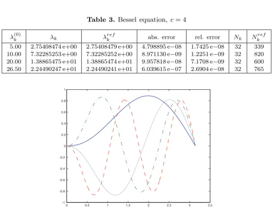
Table 3.Bessel equation, c= 4
λ(0)k λk λrefk abs. error rel. error Nk Nkref
5.00 2.75408474 e+00 2.75408479 e+00 4.798895 e−08 1.7425 e−08 32 339 10.00 7.32285253 e+00 7.32285252 e+00 8.971130 e−09 1.2251 e−09 32 820
20.00 1.38865475 e+01 1.38865474 e+01 9.957818 e−08 7.1708 e−09 32 600 26.50 2.24490247 e+01 2.24490241 e+01 6.039615 e−07 2.6904 e−08 32 765
Fig. 1.Eigenfunctions for the Bessel equation, c= 3: y1 – solid line, y2 – dotted line,
y3 – dashed-dotted line,y4 – dashed line
The next model equation, cf. [19], has the form
̺′′
(r) +n−1 r ̺
′
(r) =λ̺(r), r∈[0, a], (25)
̺(a) = 0, ̺′
(0) = 0, (26)
withn= 3anda= 1. Here, the exact eigenvalues are known to satisfyλ⋆
k=−(kπ)2,
k ∈ N. The problem is singular with a singularity of the first kind. In order to
derive the associated first order system we apply the so-called Euler transformation (z1(r), z2(r))T := ̺(r), r̺′(r)
T
x(r)we obtain the augmented first order system,
z′ (r) = 1
r
0 1 0 0 0 −1 0 0 0 0 0 0 0 0 0 0
z(r) + 0 r z3(r)z1(r)
0 z2 1(r)
, r∈(0,1],
0 0 0 0 0 1 0 0 0 0 0 1 0 0 0 0
z(0) +
1 0 0 0 0 0 0 0 0 0 0 0 0 0 0 1
z(1) = 0 0 0 1 .
The approximations for the eigenvalues are displayed in Table 4, the associated eigenfunctions can be found in Figure 2.
Table 4. Model problem from [19]:a= 1, n= 3
λ(0)k λk λ⋆k abs. error rel. error Nk
−10.00 −9.86960440 e+00 −9.86960440 e+00 9.848122 e−12 9.9782 e−13 32
−39.48 −3.94784177 e+01 −3.94784176 e+01 1.010882 e−07 2.5606 e−09 32 −90.00 −8.88264376 e+01 −8.88264396 e+01 2.052493 e−06 2.3107 e−08 32
−158.00 −1.57913672 e+02 −1.57913670 e+02 1.179932 e−06 7.4720 e−09 32
−245.00 −2.46740123 e+02 −2.46740110 e+02 1.255438 e−05 5.0881 e−08 32
Fig. 2.Eigenfunctions for the model problem from [19]: y1 – solid line,y2 – dotted line,
y3 – dashed-dotted line,y4 – dashed line,y5 – fine dotted line
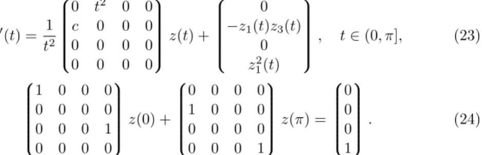
The final test problem is the so-called Boyd equation, see [9],
−y′′ (t)−1
ty(t) =λy(t), t∈(0,1], (27)
The augmented first order formulation now reads:
z′ (t) = 1
t
0 1 0 0
−t 1 0 0 0 0 0 0 0 0 0 0
z(t) + 0
−t z3(t)z1(t) 0 z2 1(t)
, t∈(0,1],
1 0 0 0 0 0 0 0 0 0 0 1 0 0 0 0
z(0) +
0 0 0 0 1 0 0 0 0 0 0 0 0 0 0 1
z(1) = 0 0 0 1 .
The numerical results are very similar to those given before, cf. Table 5 and Figure 3.
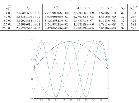
Table 5.Boyd equation
λ(0)k λk λrefk abs. error rel. error Nk Nkref
1.00 7.37398502 e+00 7.37398502 e+00 3.559406 e−09 4.8270 e−10 32 153 40.00 3.63360196 e+01 3.63360196 e+01 5.270783 e−08 1.4506 e−09 32 267 80.00 8.52925811 e+01 8.52925821 e+01 9.478771 e−07 1.1113 e−08 32 425
155.00 1.54098619 e+02 1.54098624 e+02 4.293315 e−06 2.7861 e−08 32 583
250.00 2.42705545 e+02 2.42705559 e+02 1.420079 e−05 5.8510 e−08 32 741
Fig. 3. Eigenfunctions for the Boyd equation:y1 – solid line,y2 – dotted line,
y3 – dashed-dotted line,y4 – dashed line,y5 – fine dotted line
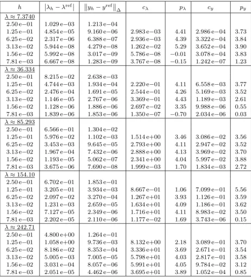
Table 6. Convergence order for the collocation solution to the Boyd equation
h ˛
˛λh−λref ˛ ˛
‚ ‚yh−yref
‚ ‚
∆ cλ pλ cy py λ≈7.3740
2.50 e−01 1.029 e−03 1.213 e−04
1.25 e−01 4.854 e−05 9.160 e−06 2.983 e−03 4.41 2.986 e−04 3.73 6.25 e−02 2.317 e−06 6.388 e−07 2.936 e−03 4.39 3.322 e−04 3.84
3.13 e−02 5.944 e−08 4.279 e−08 1.262 e−02 5.29 3.652 e−04 3.90
1.56 e−02 5.992 e−08 3.017 e−09 5.786 e−08 −0.01 3.078 e−04 3.83 7.81 e−03 6.667 e−08 1.283 e−09 3.767 e−08 −0.15 1.242 e−07 1.23 λ≈36.334
2.50 e−01 8.215 e−02 2.638 e−03
1.25 e−01 4.744 e−03 1.934 e−04 2.220 e−01 4.11 6.558 e−03 3.77 6.25 e−02 2.476 e−04 1.691 e−05 2.544 e−01 4.26 5.169 e−03 3.52
3.13 e−02 1.146 e−05 2.767 e−06 3.369 e−01 4.43 1.189 e−03 2.61 1.56 e−02 1.128 e−06 1.886 e−06 2.697 e−02 3.35 9.988 e−06 0.55 7.81 e−03 1.839 e−06 1.853 e−06 1.350 e−07 −0.70 2.034 e−06 0.03 λ≈85.293
2.50 e−01 6.566 e−01 1.304 e−02
1.25 e−01 5.976 e−02 1.102 e−03 1.514 e+00 3.46 3.086 e−02 3.56
6.25 e−02 3.453 e−03 9.645 e−05 2.793 e+00 4.11 2.947 e−02 3.52
3.13 e−02 1.967 e−04 7.432 e−06 2.888 e+00 4.13 3.969 e−02 3.70 1.56 e−02 1.193 e−05 5.062 e−07 2.341 e+00 4.04 5.997 e−02 3.88 7.81 e−03 3.675 e−06 7.690 e−08 1.999 e−03 1.70 1.834 e−03 2.72 λ≈154.10
2.50 e−01 6.702 e−01 1.853 e−01
1.25 e−01 3.205 e−01 3.934 e−03 8.667 e−01 1.06 7.099 e−01 5.56
6.25 e−02 2.097 e−02 3.270 e−04 1.267 e+01 3.93 1.126 e−01 3.59
3.13 e−02 1.231 e−03 2.659 e−05 1.634 e+01 4.09 1.186 e−01 3.62 1.56 e−02 7.127 e−05 2.349 e−06 1.716 e+01 4.11 8.983 e−02 3.50 7.81 e−03 2.202 e−05 2.110 e−06 1.177 e−02 1.69 3.743 e−06 0.15
λ≈242.71
2.50 e−01 4.800 e+00 1.264 e−01
1.25 e−01 1.058 e+00 9.736 e−03 8.132 e+00 2.18 3.089 e−01 3.70
6.25 e−02 8.186 e−02 8.353 e−04 3.336 e+01 3.69 2.671 e−01 3.54 3.13 e−02 5.005 e−03 7.005 e−05 5.798 e+01 4.03 2.817 e−01 3.58 1.56 e−02 3.031 e−04 8.057 e−06 5.991 e+01 4.05 9.784 e−02 3.12 7.81 e−03 2.051 e−05 4.462 e−06 3.695 e+01 3.89 1.052 e−04 0.85
The norm of the absolute error for an eigenfunctionyh(t),
yh−yref
∆, has been
calculated by taking a discrete maximum of
yh(t)−yref(t)
from its evaluation at
1,000 equidistantly spaced points in the interval of integration. In order to estimate the error constantc and the convergence orderp, we have assumed that the stepsize his small enough to justify the following asymptotic behavior:
|λh−λ⋆|=cλhpλ, kyh−y⋆k∞=cyh
py.
Using the data associated with two consecutive grids, we were able to provide the approximations for the values cλ, pλ and cy, py. In Table 6, the order p= 4 both
observed. Note that the accuracy of the reference solution constitutes a limitation for the range of observability of the convergence order.
REFERENCES
[1] Ascher U., Christiansen J., Russell R. D.,Collocation software for boundary value ODEs, ACM Transactions on Mathematical Software7(1981) 2, 209–222.
[2] Ascher U., Mattheij R. M. M., Russell R. D.,Numerical solution of boundary value problems for ordinary differential equations, Prentice-Hall, Englewood Cliffs, NJ, 1988.
[3] Auzinger W., Kneisl G., Koch O., Weinm¨uller E.,A collocation code for boundary value problems in ordinary differential equations, Numer. Algorithms33 (2003), 27–39.
[4] Auzinger W., Koch O., Praetorius D., Weinm¨uller E., New a posteriori error estimates for singular boundary value problems, Numer. Algorithms40 (2005), 79–100.
[5] Auzinger W., Koch O., Weinm¨uller E., Collocation methods for boundary value problems with an essential singularity, Large-Scale Scientific Computing (I. Lir-kov, S. Margenov, J. Wasniewski, and P. Yalamov, eds.), Lecture Notes in Computer Science, vol. 2907, Springer Verlag, 2004, 347–354.
[6] , Analysis of a new error estimate for collocation methods applied to singular boundary value problems, SIAM J. Numer. Anal. 42 (2005) 6, 2366– 2386.
[7] ,Efficient mesh selection for collocation methods applied to singular BVPs, J. Comput. Appl. Math. 180(2005), no. 1, 213–227.
[8] Bailey P. B., Everitt W. N., Weidmann J., Zettl A., Regular approximations of singular Sturm-Liouville problems, Results Math. 23 (1993), 3–22.
[9] Bailey P. B., Everitt W. N., Zettl A.,Computing eigenvalues of singular Sturm-Liouville problems, Results Math.20 (1991), 391–423.
[10] , Regular and singular Sturm-Liouville problems with coupled boundary conditions, Proc. Roy. Soc. Edinburgh Sect. A 126(1996), 505–514.
[11] de Hoog F. R., Weiss R.,Difference methods for boundary value problems with a singularity of the first kind, SIAM J. Numer. Anal.13 (1976), 775–813.
[12] , On the boundary value problem for systems of ordinary differential equations with a singularity of the second kind, SIAM J. Math. Anal.11 (1980), 41–60.
[14] Koch O.,Asymptotically correct error estimation for collocation methods applied to singular boundary value problems, Numer. Math. 101(2005), 143–164.
[15] Kreiss H.-O., Difference approximations for boundary and eigenvalue problems for ordinary differential equations, Math. Comp.26(1972) 119, 605–624.
[16] Naimark M. A.,Linear Differential Operators, vol. II, Ungar, New York, 1968.
[17] Pryce J., Numerical solution of Sturm-Liouville problems, Oxford University Press, New York, 1993.
[18] Shampine L., Kierzenka J., A BVP solver based on residual control and the MATLAB PSE, ACM T. Math. Software 27(2001), 299–315.
[19] Smiley M. W.,Time-periodic solutions of nonlinear wave equations in balls, Oscil-lation, Bifurcation and Chaos, CMS Conference Proceedings, vol. 8, Canadian Mathematical Society, 1987, 287–297.
Winfried Auzinger
Vienna University of Technology
Institute for Analysis and Scientific Computing Wiedner Hauptstrasse 8–10/101, A-1040 Wien [email protected]
Ernst Karner
Vienna University of Technology
Institute for Analysis and Scientific Computing Wiedner Hauptstrasse 8–10/101, A-1040 Wien [email protected]
Othmar Koch
Vienna University of Technology
Institute for Analysis and Scientific Computing Wiedner Hauptstrasse 8–10/101, A-1040 Wien [email protected]
Ewa Weinm¨uller
Vienna University of Technology
Institute for Analysis and Scientific Computing Wiedner Hauptstrasse 8–10/101, A-1040 Wien [email protected]
![Fig. 2. Eigenfunctions for the model problem from [19]: y 1 – solid line, y 2 – dotted line, y 3 – dashed-dotted line, y 4 – dashed line, y 5 – fine dotted line](https://thumb-eu.123doks.com/thumbv2/123dok_br/16301461.186128/9.892.183.704.497.887/eigenfunctions-model-problem-dotted-dashed-dotted-dashed-dotted.webp)