Adaptive Collocation Methods for the Solution of
Partial Differential Equations
Paulo Brito
Dept. of Chemical and Biological Technology, School of Technology and Management, Polytechnic Inst. of Bragança
Campus de Santa Apolónia, Apartado 1134 5301-857 Bragança - Portugal
António Portugal
Dept. of Chemical Engineering, Faculty of Sciences and Technology, University of Coimbra
Pólo II, Rua Sílvio Lima 3030-790 Coimbra - Portugal
Abstract
—
Anintegration algorithm that conjugates a Method ofLines (MOL) strategy based on finite differences space discretizations, with a collocation strategy based on increasing level dyadic grids is presented. It reveals potential either as a grid generation procedure and a Partial Differential Equation (PDE) integration scheme. It copes satisfactorily with a example characterized by a steep travelling wave and a example that presented a forming steep shock, which demonstrates its versatility in dealing with different types of steep moving front problems, exhibiting features like advection-diffusion, widely common in the standard Chemical Processes simulation models.
Keywords-Partial Differential Equation; Numerical Methods; Adaptive Methods; Collocation Methods; Dyadic Grids
I. INTRODUCTION
One can state that the main purpose of science is to contribute for the understanding of the physical phenomena that surround us. Therefore, in order to achieve this goal, scientific researchers apply the so called scientific method that can be resumed as:
• Use of experience and data available for recognition of problems that need to be solved.
• Formulation of hypothesis that potentially would solve the problem detected.
• Gathering of information in order to test the hypothesis formulated.
• Confirmation or rejection of the hypothesis formulated by the analysis of former or new data obtained.
The generally explanatory hypothesis can be simply a model, or more precisely, a mathematical model, that resume the observed phenomena on more easily treatable relations between abstract entities trough mathematical operations. In the field of mathematical models, one can narrow even more the scope of interest to problems defined over space-time continuous domains, where phenomena are not only affected by the values of the variables that define its state, but also by the gradients of these variables in relation to the independent coordinates. In the latter case, the mathematical models are necessarily constituted by differential (or integral) equations defined on multidimensional domains, i.e., partial differential equations (PDE’s). However, the process of constructing a suitable model, or modelling, has to be complemented with the not less important task of solving it efficiently.
II. NUMERICAL METHODS
It is clear that it is not always possible to solve mathematical problems using analytic procedures. In these cases (usually non-linear problems), one has to resort to numerical analysis, the study of algorithms, i.e. sequential operation schemes that generally imply a discretization of continuous defined problems. These schemes can be applied in the solution of a variety of mathematical problems, such as optimization, calculation of integrals, interpolation, resolution of algebraic or differential equations, etc. Our interest resides on the numerical methods for the solution of time dependent partial differential equations (or systems of equations) defined over one- or multidimensional space domains. These schemes usually imply the construction of discrete grids that cover the total domain, and the approximation of the continuous solution by basis functions. The most important classes of numerical methods developed for the solution of PDE’s differ between each other by the type of basis functions chosen, e.g.:
• Finite Differences (FD) – Taylor expansion series.
• Finite Elements (FE) – Interpolating polynomials.
• Spectral – Orthogonal Functions. A. Method of Lines
B. Adaptation Concept
The classical approach to these kind of procedures is generally rigid and not adaptable to its evolution. One way to turn around the problems that may arise from the lack of flexibility of that approach is the introduction of the adaptation concept. Adaptivity implies the adjustment of algorithm parameters to the particular circumstances of the solution evolution. In the field of numerical solution of PDE´s it can assume the following purposes:
• h-refinement – grid refinement and relaxation.
• p-refinement – adjustment of approximating orders.
• r-refinement – introduction of nodal velocities. These strategies are not mutually exclusive and may be combined in mixed adaptive methods. The application of adaptivity in the PDE solving field has already several decades, and the number and variety of methods proposed is rather extensive [5,6]. However, the primordial objectives of the adaptive procedure are generally the same: the construction of grids that concentrate nodes in the domain regions where the solution is more active (i.e. shows steeper gradients) and disperse them in the remaining regions, and follow efficiently the problematic features of the solution. The application of adaptivity into the MOL strategy concept is straightforward [7].
C. Dyadic Grids
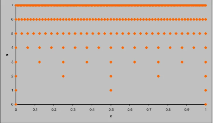
We chose to construct grids at each time step of the integration, based in a series of embedded one-dimensional dyadic grids of decreasing level. A k-level one-dimensional dyadic grid is defined by a nodal mesh with 2k intervals. Obviously, in a correspondent uniform grid, the size of a k -level grid is constant through the total domain. A higher -level grid is constructed by adding nodes to the immediately previous one, at every interval middle position (Fig. 1).
Fig. 1. Uniform dyadic grids of increasing level n.
It is important to note that a grid of level k is always included in all grids of higher level. So, the purpose is to generate grids that combine nodes of different levels according to the function activity at the various regions of the domain. It is obvious that the presented strategy can be easily extended to multidimensional domains.
For that purpose, we define a collocation strategy that uses function dependent features, to allow the activation (or deactivation) of nodes belonging to dyadic grids ranging from the lower resolution level (M) – the basis level; to a maximum allowed resolution level (N).
D. Numerical Algorithm
Applying the dyadic grid concept with finite differences approximations, we devise a collocation algorithm for grid generation which can be applied in MOL algorithm for the solution of PDE’s. Considering a region of space domain defined by two consecutive dyadic grids (Fig. 2), a collocation algorithm is developed for activating the required nodes by the procedure described below.
Collocation Algorithm
• k = M
• for i =1, …, 2k –1
• estimate n i
U (order n derivative at node i) by finite differences
• if collocation criterion is met: select intermediate nodes
of level k+1: 1
1 2 1 2 1
1
2 ; ;
+ + + +
− ki
k i k
i x x
x
• k = k +1 (repeat fork = M, …, N –1)
xk i xk
i-1 xki+1
... ...
k k+1 xk+1
2i xk+1
2i-1 xk+12i+1
Fig. 2. Representation of the connection between nodes of consecutive levels.
The collocation criterion obeys to two different strategies. First, the grid size is calculated by,
2 1 1
k i k i x
x x= + − −
∆ , (1)
Then, we define a criterion that captures oscillations on the finite difference estimate profile:
Criterion I
• calculate in
n i U
U 1
1= × −
δ and in
n i U
U ×
= +1 2
δ
• criterion verified if:
1
ε
> ∆
× x
Un
i or
≤ ≤
0 0
2 1
δ δ
and 2
1 1
3 >ε
+
+ +
− in
n i n
i U U
U
Additionally, a second criterion that tracks high variations on the finite difference estimate profile is defined:
0 1 2 3 4 5 6 7
0 0.1 0.2 0.3 0.4 0.5 0.6 0.7 0.8 0.9 1
x
Criterion II
• calculate in
n i U
U 1
1= − −
δ and in
n i U
U −
= +1
2
δ
• criterion verified if:
1
ε
> ∆
× x
Uin or δ1×δ2 ≤0
and 2
2 1
2 ε
δ δ + >
ε1 and ε2 represent the criteria tolerances. Both criteria tend to
take advantage of the approximating nature of the space derivatives estimating scheme. The errors associated with the finite difference procedure induce artificial oscillations in the estimated derivative profiles mainly near the steep fronts regions, which can be identified. Therefore, we increase the grid resolution on these regions by activation of higher level nodes that do not verify the more demanding collocation criteria. The gathering of all active nodes in every dyadic grid, generate the overall grid. One advantage of this procedure is the possibility of applying the collocation algorithm sequentially, analyzing several derivative orders by stages, e.g. generating a grid that verify the first derivative condition and subsequently running the obtained grid through a second derivative analysis.
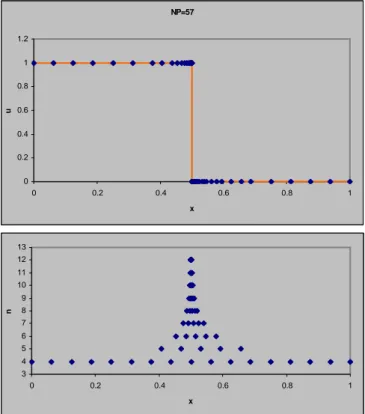
Fig. 3. Grid generated for the Step Function.
III. GRID GENERATION
First, we tested the performance of the collocation algorithm for the generation of grids that conform to the properties of selected one-dimensional functions.
A. Example 1 – Step Function
A simple function that represents a one-dimensional negative space step, i.e. a discontinuity located at the middle position of the domain [0,1],
( )
( )
≤ ≤ =
< ≤ =
1 5 . 0 , 0
5 . 0 0 , 1
x x
u
x x
u
, (2)
is tested using the collocation criterion I. We analyse the finite difference approximation (5 nodes centred) of the first derivative, with ε1 = ε2 = 0.1. The basis grid of lowest level is
a uniform grid with 24 intervals and the highest dyadic grid level is N=12. The grid generated is presented in Fig. 3. We observe that the algorithm is able to detect the discontinuity quite satisfactorily and the constructed grid is adequate to represents the function main features with a reasonable total number of nodes (NP=57).
B. Example 2 – TGH Function
Now, we try to represent in a discrete fashion a function characterised by a very steep front located at the middle of the domain, surrounded by two flat plateaus at each side. The function is defined by the following hyperbolic tangent:
( )
x =tanh(
60x−0.01)
u . (3)
Again, it is applied the collocation criterion I, by the analysis of the finite difference approximation (5 nodes centred) of the first derivative, with ε1 = ε2 = 0.1, M=4 and N=12. The results
are resumed in Fig. 4. We conclude that the front is easily tracked and the generated grid allows the representation of the by a reasonable total number of nodes (NP=58).
The algorithm proves to be able to generate grids that efficiently detect and represent steep features in the studied functions.
IV. SIMULATION EXPERIMENTS
The node collocation procedure is incorporated in an algorithm for the resolution of one-dimensional time-dependent PDE´s. This strategy is based on the conjugation of a MOL algorithm where the space derivatives are approximated by finite differences formulas, with grid generation procedure at specified times that reformulate the space grid according to the solution evolution. At these intermediate times the solution profiles are reconstructed through an interpolation scheme. The time integration is performed by the ODE integrator DASSL. Therefore the presented algorithm can be included in the class of h-refinement PDE solution adaptive procedures.
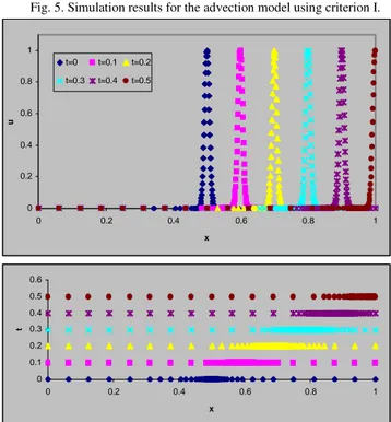
A. Model 1 – Advection Equation
We test the integration algorithm using a very simple equation known as the advection equation,
3 4 5 6 7 8 9 10 11 12 13
0 0.2 0.4 0.6 0.8 1
x
n
NP=57
0 0.2 0.4 0.6 0.8 1 1.2
0 0.2 0.4 0.6 0.8 1
x
Fig. 4. Grid generated for the TGH Function.
x u v t u
∂ ∂ − = ∂
∂ , (4)
defined over the domain x∈ [0,1], with the boundary condition,
u
( )
0,t =0. (5)In spite of its apparent simplicity, the solution of this equation can be rather problematic, depending on the initial conditions chosen. The solution space wave is propagated through time without distortion, with velocity ν in the positive direction of the x referential. If the initial profile exhibits a steep front, the adequate numerical translation of the continuous problem by a uniform fixed grid, may prove to be difficult. So, we use the function,
( )
(
)
−
− =
ε
2 0 exp
0
, x x
x
u , (6)
TABLE I. SIMULATION PARAMETERS FOR MODEL 1
Collocation criterion I or II
Derivative order for collocation n=1 and 2; or n=1
Time step 10-3
Finite Difference approximation 5 nodes centred - uniform grid
Interpolation strategy Cubic splines with 9 nodes
Time integrator tolerances 10-6
Dyadic grids levels M=4; N=10
ε1 = ε2 =10-2
with x0 = 0.5 and ε = 1×10⁻⁴, which represents a steep wave to
test the algorithm performance in the conditions described in Table I.
The results obtained are resumed in Fig. 5 and 6, using criterion I and II, respectively. It is observed that the algorithm provides rather good results, providing a close track of the wave propagation until it collides to the right boundary. The results obtained with the two criteria appear to be very similar.
Fig. 5. Simulation results for the advection model using criterion I.
Fig. 6. Simulation results for the advection model using criterion II.
0 0.1 0.2 0.3 0.4 0.5 0.6
0 0.2 0.4 0.6 0.8 1
x
t
0 0.2 0.4 0.6 0.8 1
0 0.2 0.4 0.6 0.8 1
x
u
t=0 t=0.1 t=0.2 t=0.3 t=0.4 t=0.5 0
0.1 0.2 0.3 0.4 0.5 0.6
0 0.2 0.4 0.6 0.8 1
x
t
0 0.2 0.4 0.6 0.8 1
0 0.2 0.4 0.6 0.8 1
x
u
t=0 t=0.1 t=0.2 t=0.3 t=0.4 t=0.5
3 4 5 6 7 8 9 10 11 12 13
-1 -0.5 0 0.5 1
x
n
NP=58
-1.2 -1 -0.8 -0.6 -0.4 -0.2 0 0.2 0.4 0.6 0.8 1 1.2
-1 -0.5 0 0.5 1
x
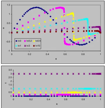
B. Model 2 – 1-D Burgers’ Equation
The second test model is the widely studied 1-D inviscid Burgers’ Equation[4],
2 2
x u v x u u t u
∂ ∂ + ∂ ∂ − = ∂
∂ , (7)
defined over the domain x∈ [0,1], with the boundary conditions:
( ) ( )
0,t =u1,t =0u . (8)
This PDE represent an advection-diffusion problem, which, depending of the initial condition applied, may present some interesting challenges. Therefore, for the initial condition,
( )
x(
x)
( )
xu π sinπ
2 1 2 sin 0
, = + , (9)
as the advection velocities are the solution itself, the problem evolves from a rather smooth profile to a steep front forming at x≈ 0,60 by t≈ 0,20. From this instant on, the front moves on the positive direction of x until it eventually crashes onto the right boundary and slowly fades away. The size of the moving front thickness depends on the importance of the diffusion term, i.e. it is proportional with the scale of the diffusion coefficient (ν). In Table II, we resume the algorithm run conditions for ν = 10-3, using both collocation criteria. The simulation results for the criterion I are condensed in Fig. 7. We conclude that the algorithm successfully follows the formation and movement of the steep, with hardly any difficulty. The results obtained using the two collocation criteria seem to be very similar.
Now, the Burgers’ equation is solved in more demanding conditions, decreasing the influence of diffusivity by fixing the parameter ν = 10-4. In these conditions, we apply the usual sequential first and second derivative analysis, associated with criterion I.
However, the maximum level grid is increased to N=12, to account to the reducing thickness of the moving steep front. The general conditions are resumed in Table III.
TABLE II. SIMULATION PARAMETERS FOR MODEL 2(ν=10-3)
Collocation criterion I or II
Derivative order for collocation n=1 and 2; or n=1
Time step 10-2
Finite Difference approximation 5 nodes centred - uniform grid
Interpolation strategy Cubic splines with 7 nodes
Time integrator tolerances 10-6
Dyadic grids levels M=4; N=10
Criterion I: ε1 = ε2 =100; Criterion II: ε1 = ε2 =10-1
Fig. 7. Simulation results for the Burgers’ model using criterion I (ν = 10-3).
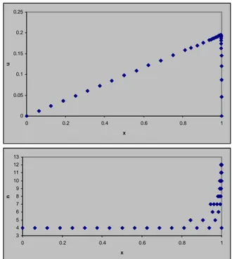
Fig. 8. Simulation results for model 2 at t=0, using criterion I (ν = 10-4).
In Fig. 8, we present the grid generation results concerning the initial condition profile. It is obvious that due to the smooth characteristics of this profile, the grid is relatively coarse and the maximum level attained is only a modest 6.
However, the situation changes radically for t=0.20 (Fig. 9). At this instant, the front is fully developed, and the procedure has to take advantage of the maximum level nodes to adequately conform to the front and its edges.
3 4 5 6 7 8 9 10 11 12 13
0 0.2 0.4 0.6 0.8 1
x
n
-1 -0.5 0 0.5 1 1.5
0 0.2 0.4 0.6 0.8 1
x
u
0 0.5 1 1.5 2 2.5 3 3.5
0 0.2 0.4 0.6 0.8 1
x
t
-1 -0.5 0 0.5 1 1.5
0 0.2 0.4 0.6 0.8 1
x
u
TABLE III. SIMULATION PARAMETERS FOR MODEL 2(ν=10-4)
Collocation criterion I
Derivative order for collocation n=1 and 2
Time step 2.5×10⁻³
Finite Difference approximation 5 nodes centred - uniform grid
Interpolation strategy Cubic splines with 7 nodes
Time integrator tolerances 10-6
Dyadic grids levels M=4; N=12
ε1 = ε2 =100
Fig. 9. Simulation results for model 2 at t=0.2, using criterion I (ν = 10-4).
Fig. 10. Simulation results for model 2 at t=1.0, using criterion I (ν = 10-4).
After the formation of the steep front, the algorithm shows its ability to follow the movement of the front without introducing numerical distortions on the edges (Fig. 10).
The algorithm also proves its suitability by providing a adequately simulation of the front crash at the right boundary (Fig. 11). In general, the simulation is successfully carried out.
Fig. 11. Simulation results for model 2 at t=1.0, using criterion I (ν = 10-4).
V. CONCLUSIONS
We conclude that the integration algorithm that conjugates a MOL strategy with finite differences space discretizations, with a collocation strategy based on increasing level dyadic grids, revealed potential either as a grid generation procedure and a PDE integration scheme. It coped satisfactorily with a example characterized by a steep travelling wave and a example that presented a forming steep shock, which proves its versatility in dealing with different types of problems.
REFERENCES
[1] W. E. Schiesser, The Numerical Method of Lines: Integration of Partial Differential Equations, Academic Press, San Diego, 1991.
[2] J.C. Santos, P. Cruz, F.D. Magalhães and A. Mendes, “2-D Wavelet-based adaptive-grid method for the resolution of PDEs,” AIChe J., vol. 49, pp. 706-717, March 2003.
[3] P. Cruz, M.A. Alves, F.D. Magalhães and A. Mendes, “Solution of hyperbolic PDEs using a stable adaptive multiresolution method,” Chem. Eng. Sci., vol. 58, pp. 1777-1792, May 2003.
[4] T.A. Driscoll and A.R.H. Heryudono, “Adaptive residual subsampling methods for radial basis function interpolation and collocation problems,” Comput Math. Appl., vol. 53, pp. 927-939, March 2007. [5] D.F. Hawken, J.J. Gottlieb and J.S. Hansen, “Review of some adaptive
node-movement techniques in finite-element and finite-difference solutions of partial differential equations,” J. Comput. Phys., Vol. 95, pp. 254-302, August 1991.
[6] P. Brito, Aplicação de Métodos Numéricos Adaptativos na Integração de Sistemas Algébrico-diferenciais Caracterizados por Frentes Abruptas, MSc. Thesis, DEQ-FCTUC, Coimbra, Portugal, 1998.
[7] A. Vande Wouwer, Ph. Saucez, and W. E. Schiesser (eds.), Adaptive Method of Lines, Chapman & Hall/CRC Press, Boca Raton, 2001.
3 4 5 6 7 8 9 10 11 12 13
0 0.2 0.4 0.6 0.8 1
x
n
0 0.05 0.1 0.15 0.2 0.25
0 0.2 0.4 0.6 0.8 1
x
u
3 4 5 6 7 8 9 10 11 12 13
0 0.2 0.4 0.6 0.8 1
x
n
-0.2 -0.1 0 0.1 0.2 0.3 0.4 0.5 0.6 0.7 0.8
0 0.2 0.4 0.6 0.8 1
x
u
3 4 5 6 7 8 9 10 11 12 13
0 0.2 0.4 0.6 0.8 1
x
n
-1 -0.5 0 0.5 1 1.5
0 0.2 0.4 0.6 0.8 1
x