ISSN 1549-3636
© 2011 Science Publications
Corresponding Author: Mohammad Hossin, Department of Computer Science, Faculty of Computer Science and Information Technology, University Putra Malaysia, 43400 Serdang, Selangor, Malaysia
A Novel Performance Metric for Building an Optimized Classifier
1,2
Mohammad Hossin, 1Md Nasir Sulaiman, 1
Aida Mustapha and 1Norwati Mustapha 1
Department of Computer Science,
Faculty of Computer Science and Information Technology, University Putra Malaysia, 43400 UPM Serdang, Selangor, Malaysia
2
Department of Cognitive Science,
Faculty of Cognitive Sciences and Human Development,
University Malaysia Sarawak, 94300 Kota Samarahan, Sarawak, Malaysia
Abstract: Problem statement: Typically, the accuracy metric is often applied for optimizing the heuristic or stochastic classification models. However, the use of accuracy metric might lead the searching process to the sub-optimal solutions due to its less discriminating values and it is also not robust to the changes of class distribution. Approach: To solve these detrimental effects, we propose a novel performance metric which combines the beneficial properties of accuracy metric with the extended recall and precision metrics. We call this new performance metric as Optimized Accuracy with Recall-Precision (OARP). Results: In this study, we demonstrate that the OARP metric is theoretically better than the accuracy metric using four generated examples. We also demonstrate empirically that a naïve stochastic classification algorithm, which is Monte Carlo Sampling (MCS) algorithm trained with the OARP metric, is able to obtain better predictive results than the one trained with the conventional accuracy metric. Additionally, the t-test analysis also shows a clear advantage of the MCS model trained with the OARP metric over the accuracy metric alone for all binary data sets.
Conclusion: The experiments have proved that the OARP metric leads stochastic classifiers such as the MCS towards a better training model, which in turn will improve the predictive results of any heuristic or stochastic classification models.
Key words: Performance metric, Optimized Accuracy with Recall-Precision (OARP), accuracy metric, extended precision, extended recall, optimized classifier, Monte Carlo Sampling (MCS)
INTRODUCTION
To date, many efforts have been carried out to design more advanced algorithms to solve classification problems. At the same time, the development of appropriate performance metrics to evaluate the classification performance are at least as importance as algorithm. In fact, it is a key point to produce a successful classification model. In other words, the performance metric plays a significant role in guiding the design of better classifier.
From the previous studies, the performance metric is normally employed in two stages (i.e., the training stage and the testing stage). The use of performance metric during the training stage is to optimize the classifier (Ferri et al., 2002; Ranawana and Palade, 2006). In other words, in this particular stage, the
performance metric is used to discriminate and to select the optimal solution which can produce a more accurate prediction of future performance. Meanwhile, in the testing stage, the performance metric is usually employed for comparing and evaluating the classification models (Bradley, 1997; Caruana and Niculescu-Mizil, 2004; Kononenko and Bratko, 1991; Provost and Domingos, 2003; Seliya et al., 2009).
selection of suitable performance metric is essential. Traditionally, most of the heuristic and stochastic classification models employ the accuracy rate or the error rate (1-accuracy) to discriminate and to select the optimal solution. However, using the accuracy metric as a benchmark measurement has a number of limitations, which have been verified by many works (Ferri et al., 2002; Ranawana and Palade, 2006; Wilson, 2001). In those studies, they have demonstrated that the simplicity of this accuracy metric could lead to the sub-optimal solutions especially when dealing with imbalanced class distribution. Furthermore, the accuracy metric also exhibits poor discriminating values to discriminate better solution in order to build an optimized classifier (Huang and Ling, 2005).
Instead of the accuracy metric, there are few other metrics which have been designed purposely to build an optimized classifier. A Mean Squared Error (MSE) is one of the popular error function metric that are used by many neural network classifiers such as back-propagation network (Al-Bayati et al., 2009; Pandya and Macy, 1996) and supervised Learning Vector Quantization (LVQ) (Kohonen, 2001) for evaluating neural network performance during the training period. In general, MSE measures the difference between the predicted solutions and desired solutions. By employing this metric, the smaller MSE value is required in order to obtain a better neural network classifier.
Meanwhile, Lingras and Butz (2007) proposed the used of extended precision and recall values to identify the boundary region for the Rough Support Vector Machines (RVSM). In this study, the notion of conventional precision and recall metrics are extended by defining separate values of precision and recall for each class. However, both of these performance metrics could not be employed by other heuristic and stochastic classification algorithms due to different learning paradigm or objective function being used.
On top of that, Ranawana and Palade (2006) introduced a new hybridized performance metric called the Optimized Precision (OP) for evaluating and discriminating the solutions. This performance metric is derived from a combination of three performance metrics, which are accuracy, sensitivity and specificity. In this study, they have demonstrated that the OP metric is able to select an optimized generated solution and is able to increase the classification performance of ensemble learners and Multi-Classifier Systems for solving Human DNA Sequences data set. Area under the ROC curve (AUC) is another popular performance metric used to construct optimized learning models (Ferri et al., 2002). In general, the AUC provides a single value for discriminating which solution is better
on average. This performance metric is proven theoretically and empirically better than the accuracy metric in optimizing the classifier models (Huang and Ling, 2005).
Similar to the above-mentioned performance metrics, the main purpose of this study is trying to improve the problem of accuracy metric in discriminating an optimal solution in order to build an optimized classifier for heuristic and stochastic classification algorithms. This study introduces a new hybridized performance metric that is derived from the combination of accuracy metric with the extended precision and recall metrics. The new performance metric is known as an Optimized Accuracy with Recall-Precision (OARP) metric. We believe that the benefits of the accuracy and extended precision and recall can be best exploited to construct a new performance metric that is able to optimize the classifier for heuristic and stochastic classification algorithms. In this study, we limit our study scope by comparing the new performance metric against the conventional accuracy metric. Moreover, the two-class classification problem is used for comparing both metrics.
Further, we will show that our proposed performance metric is better than the conventional accuracy metric by constructions of examples from different types of class distribution in discriminating the optimal solution. Next, with more discriminating features and finer measure, we will show that any heuristic or stochastic classification algorithm would search better and later obtain better optimal solution. A series of experiment using nine real data sets will be used to demonstrate that the Monte Carlo Sampling (MCS) algorithm optimized by the OARP metric produce better predictive result as compared to the algorithm optimized by the accuracy metric alone.
MATERIALS AND METHODS
Related performance metrics: The performance evaluation for binary classification model is based on the count of correctly and incorrectly predicted instances. These counts can be tabulated in a specific table known as a confusion matrix. In the confusion matrix, the counts of predicted instances can be categorized into four categories. Table 1 shows the four categories of results of confusion matrix.
Table 1: Confusion matrix
Actual positive Actual negative
Predicted positive tp fp
Predicted negative fn tn
positive patterns that are misclassified as negative class. Through these four categories of results, few performance metrics have been derived from the literature as below.
Accuracy (Acc): Accuracy measures the fraction of positive and negative patterns which are correctly classified by the classifier:
tp Acc
tp fp tn fn =
+ + + (1)
Sensitivity (Sn): Sensitivity measures the fraction of positive patterns being correctly classified as positive class:
tp Sn
tp fn =
+ (2)
Specificity (Sp): Specificity measures the fraction of negative patterns being correctly classified as negative class:
tn Sp
tn fp =
+ (3)
Recall (r): The function of this metric is similar to sensitivity metric:
tp r
tp fn =
+ (4)
Precision (p): Precision is used to determine the fraction of patterns that predicted to be positive in a positive class:
tp p
tp fp =
+ (5)
On top of the above-mentioned metrics, few advanced metrics are also proposed based on the confusion matrix as a reference. Below we discussed two advanced metrics which are related to our study.
Optimized Precision (OP): Ranawana and Palade (2006) proposed a new hybridized metric called the Optimized Precision (OP). This new metric is a combination of three performance metrics which are accuracy, sensitivity and specificity. In order to construct this hybridized metric, a new measurement
called Relationship Index (RI) is introduced with the objective to minimize the value of |Sp-Sn| and at the same time to maximize the value of Sp+Sn. The RI is defined as in Equation 6. A high value of RI would entail a low |Sp-Sn| value and a high value of Sp+Sn:
Sp Sn RI
Sp Sn − =
+ (6)
In order to apply Equation 6 in the performance of optimization algorithms, Ranawana and Palade (2006) combine the beneficial properties of accuracy and RI as shown in Eq. 7 to reduce the detrimental effect of data split during training of the classifier. Through this combination, the value of OP remains relatively stable even when presented with large imbalanced class distribution:
Sp Sn OP Acc RI Acc
Sp Sn −
= − = −
+ (7)
In the case of RI = 0 when Sp = Sn, an alternative definition of OP was proposed as given in Eq. 8:
Sp Sn Sp Sn Sn Sp Sn Sp
Acc ;if Sn Sp
OP Acc ;if Sp Sn
Acc ;if Sn Sp
− + − + ⎧
⎪ =
⎪ ⎪
=⎨ − >
⎪ ⎪
− >
⎪ ⎩
(8)
Extended version of precision and recall:
Nonetheless, binary classifier only deals with ‘yes’ and ‘no’ answers for a single class. In other words, the classifier is trying to separate the instances into two different classes, which are either class 1 or class 2. Through this concept, Lingras and Butz (2007) propose an extended version of precision and recall by defining precision and recall for each class.
Let assume for two-class problem every class has their own precision and recall value C1= {p1, r1},
C2={p2, r2}, a set of instances that belongs to each class
C1= {R1}, C2={R2}, as well as a set of predicted
instances C1= {A1}, C2={A2}. Having these properties,
the extended precision and recall for two-class problem can be defined as in Eq. 9 and 10 respectively:
i i
i i
R A
p A
∩
= (9)
i i
i
i
R A
r R
∩
where, 1≤i≤c and c is the maximum number of class. Lingras and Butz, (2007), they have theoretically proved that for two-class problem the precision of one class is correlated to the recall of other class for two-class problem. This correlation can be defined as p1 is proportional to r2 (p1∝r2) and p2 is proportional to r1 (p2∝r1). Through this correlation, they demonstrated that these extended precision and recall values can be used to identify the boundary region (lower bound for both classes) for the Rough Support Vector Machines (RVSMs) instead of using conventional hyper plane.
The optimized accuracy with recall-precision: The aim of most classification model is to maximize the total number of correct predicted instances in every class. In certain situation, it is hard to produce a classifier which can obtain the maximal value for every class. For instance, when dealing with imbalanced class instances, it is often happen where the classification model is able to perform extremely well on a large class instances but unfortunately perform poorly on the small class instances. Clearly, this indicates that the main objective of any classification model should be maximizing all class instances in order to build an optimized classifier.
As mentioned earlier, the accuracy metric is often used to build and to evaluate an optimized classifier. However, the use of accuracy value could lead the searching and discriminating processes to the sub-optimal solutions due to its poor discriminating feature. Moreover, the metric is also not robust when dealing with imbalanced class instances. This observation will be experimentally demonstrated in the next sub-section. In contrast, precision and recall are two performance metrics that are used as alternative metrics to measure the binary classifier performance from two different aspects. In any binary classification problem, it is possible that for the classifier to produce higher training accuracy with higher precision value but lower recall value or with lower precision value but higher recall value. As a result, building a classifier that maximizes both precision and recall values is the key challenge for many binary classifiers. However, it is difficult to apply both of these metrics separately. By applying these metrics separately, it will cause the selection and discrimination processes become difficult due to multiple comparisons.
We believe that the beneficial properties of accuracy, precision and recall metrics can be exploited to construct a new performance metric that is more discriminating, stable and robust to the changes of class distribution. In order to transform these metrics into a singular form of metric, we will adopt two important
formulas from (Ranawana and Palade, 2006), which are the Relationship Index (RI) and OP. This is a two-step effort, whereby first we have to find a suitable way to employ the RI formula and next to identify the best approach to adopt the OP formula in order to construct the new performance metric.
From our point of view, the conventional precision and recall metrics are not suitable for the integration process. This is because both metrics only measure one class of instances (positive class). This is somewhat against the earlier objective which attempts to maximize every class instances in order to build an optimized classifier. To resolve this limitation, the extended precision and recall metrics proposed by (Lingras and Butz, 2007) were suggested for the integration. The main justification is that every class instance should be able to be measured individually using both metrics as defined in Equation 9 and Equation 10.
As proved by (Lingras and Butz, 2007), for two-class problem, the extended precision value in a particular class is proportional to the extended recall values of the other class and vice versa. From this correlation, the RI formula can be implemented. To employ the RI formula, the precision and recall from different classes were paired together (p1, r2), (p2, r1)
based on the correlation given in (Lingras and Butz, 2007). At this point, the aim is to minimize the value of |p1-r2| and |p2-r1| and maximize the value of p1+r2 and
p2+r1. Hence, we define the RI for both correlations as
stated in Eq. 11 and 12:
1 2 1
1 2
p r RI
p r − =
+ (11)
2 1 2
2 1
p r RI
p r − =
+ (12)
However, these individual RI values are still pointless and could not be applied directly to calculate the value of new performance metric. Thus, to resolve this problem, we compute the average of total RI (AVRI) as shown in Eq. 13 to formulate the new performance metric:
c
i i 1
1
AVRI RI
c =
=
∑
(13)to deal with imbalanced class distribution. Such drawbacks motivate us to combine the beneficial properties of AVRI with the accuracy metric. With this combination, we expect the new performance metric is able to produce better value (more discriminating) than the accuracy metric and at the same time remain relatively stable when dealing with imbalanced class distribution.
The new performance metric is called the Optimized Accuracy with Recall-Precision (OARP) metric. The computation of this OARP metric is defined in Eq. 14:
OARP = Acc-AVRI (14)
However, during the computation of this new metric, we noticed that the value of OARP may deviate too far from the accuracy value especially when the value of AVRI is larger than accuracy value. Therefore, we proposed to resize the AVRI value into a small value before computing the OARP metric. To resize the AVRI value, we employed the decimal scaling method to normalize the AVRI value as shown in Eq. 15:
old _ val new _ val x
AVRI AVRI
10
= (15)
where, x is the smallest integer such that max (|AVRInew_val|) < 1.
In this study, we set the x=1 for the entire experiments. By resizing the AVRI value, we found that the OARP value is comparatively close to the accuracy value as shown in the next sub-section.
At the end, the objective of OARP metric is to optimize the classifier performance. A high OARP value entails a low value of AVRI which indicates a better generated solution has been produced. We also noticed that via this new performance metric, the OARP value is always less than the accuracy value (OARP < Acc). The OARP value will only equal to the accuracy value (OARP = Acc) when the AVRI value is equivalent to 0 (AVRI = 0), which indicates a perfect training classification result (100%).
OARP vs. accuracy: Analysis on discriminating an optimized solution: In this study, we also attempt to demonstrate that the new performance metric is better than the conventional accuracy metric through three criteria. The first criterion is that the metric has to be more discriminative. The second criterion is that the metric favors the minority class instances when majority class instances always dominate the selection process. The third criterion is that the metric is robust to the changes of class distribution. To prove these criteria, four different examples have been used to demonstrate the capability of this new performance
metric in selecting and discriminating the optimized solution based on different types of class distributions. However, in this study, we restricted our attention to the two-class classification problem suitable with the proposed metric. We also restricted our discussion to the solutions that are indistinguishable according to accuracy value (Example 1-3). On top of that, we also included one special example that shows the drawback of accuracy in discriminating the solution that has poor results on the minority class of instances but produce higher accuracy rate with the other solution that has slightly lower accuracy value but able to predict correctly all minority class of instances (Example 4).
Example 1: Given balanced data set containing 50 positive and 50 negative instances (domain Ψ) and two performance metrics, Acc and OARP are used to discriminate two similar solutions a and b, Acc={(a,b)|a,bא Ψ} and OARP={(a,b)|a,bא Ψ}. Assume that a and b obtained the same total correct predicted instances (TC) as given in Table 2a.
From this example, we can intuitively say that b is better than a. This is proved by evaluating the misclassification instances for both classes, the fp and fn for b, which are comparatively balanced as compared to a. For this case, the OARP metric showed a decision value that similar to intuitive decision, while the accuracy metric unable to decide which solution is better due to poor discriminative value.
Example 2: Given an imbalanced data set containing 70 positive and 30 negative instances (domain Ψ) and two performance metrics, Acc and OARP are used to discriminate two similar solutions a and b, Acc={(a,b)|a,bא Ψ} and OARP={(a,b)|a,bא Ψ}. Assume that a and b obtained the same total correct predicted instances (TC) as given in Table 2b.
Table 2a: Accuracy Vs. OARP for balanced data set
s tp fp tn fn TC Acc OARP
a 49 4 46 1 95 0.950000 0.949845
b 48 3 47 2 95 0.950000 0.949947
Table 2b: Accuracy Vs. OARP for imbalanced data set
s tp fp tn fn TC Acc OARP
a 69 4 26 1 95 0.950000 0.947249
b 68 3 27 2 95 0.950000 0.947384
Table 2c: Accuracy Vs. OARP for extremely imbalanced data set
s tp fp tn fn TC Acc OARP
a 94 4 1 1 95 0.950000 0.900822
b 93 3 2 2 95 0.950000 0.913032
Table 2(d): Accuracy vs. OARP: Special case
s tp fp tn fn TC Acc OARP
a 89 0 5 6 94 0.940000 0.922669
Similar to Example 1, intuitively b is better than a in terms of the fp and fn values. In this example, the OARP metric demonstrated better value and produced decision similar to intuitive decision. Meanwhile, the accuracy metric could not tell the difference between a and b.
Example 3: Given an extremely imbalanced data set containing 95 positive and 5 negative instances (domain Ψ) and two performance metrics, Acc and OARP are used to discriminate two similar solutions a and b, Acc={(a,b)|a,bא Ψ} and OARP={(a,b)|a,bא Ψ}. Assume that a and b obtained the same total correct predicted instances (TC) as given in Table 2c.
Similar to the two examples earlier, intuitively b is better than a in terms of fp and fn. As indicated in the table, the OARP metric once again able to produced decision similar to intuitive decision. However, the value of accuracy metric is unvarying and could not distinguish which solution is better.
Example 4: Given two special cases of solutions a and b and added into an extremely imbalanced data set containing 95 positive and 5 negative instances(domain Ψ) and discriminated by two performance metrics, Acc and OARP, Acc={(a,b)|a,bאΨ} and OARP={(a,b)|a,bא Ψ}. Assume that a and b obtained the same total correct predicted instances (TC) as given in Table 2d.
In this special case, two contradictory results are obtained. The accuracy metric distinguished that b is better than a, but the OARP metric resulted otherwise. Intuitively, we can conclude that a is better than b. This is because, a able to predict correctly all the minority class instances as compared to b. Clearly, b is poor since no single instance from minority class instances is correctly predicted by b. Hence, we can conclude that the result obtained by OARP metric is similar to intuitive decision and clearly better than the accuracy metric.
From the four examples given, three conclusions can be drawn from the results. First, the value of the OARP metric is more discriminating than the value of accuracy metric because the OARP metric is able to tell the difference between both solutions through the values obtained, while the accuracy metric could not. Second, these examples showed that the accuracy metric is not robust to the changes of class distribution because the size of instances changes the value of accuracy metric is no longer able to perform optimally (Example 2-4). This indicates that the accuracy metric is not a good evaluator and optimizer to be used for discriminating the optimal solution. In contrast, the OARP metric is sensitive to the changes of class distribution. Although the OARP metric is sensitive, the value produced by the OARP metric is robust and able to perform optimally by producing a clear optimal solution.
Third, when dealing with the imbalanced or extremely imbalanced class distribution, the OARP metric favored to the minority class distribution instead of majority class distribution as shown in Example 4. This criterion is really important to prove that the chosen generated solution is capable to classify minority class instances correctly. In contrast, the accuracy metric is neutral to the changes due to poor informative feature about the proportion of instances in both classes. Neutral is used here to indicate that the accuracy metric only cares with the total of correct predicted instances. The dangerous of this situation is (Example 4) it could lead the selection process of any classifier to the sub-optimal solutions.
Experimental setup: We have theoretically showed that the new performance metric, OARP was better than the accuracy metric in selecting and discriminating better solutions using four examples. Next, we are going to demonstrate the generalization capability of the OARP metric against the accuracy metric using real world application data sets.
For the purpose of comparison and evaluation on the generalization capability of OARP metric against the accuracy metric, nine binary data sets from UCI Machine Learning Repository were selected. All of these selected data sets are imbalanced class distribution. The brief descriptions about the selected data sets are summarized in Table 3.
In pre-processing data, all data sets have been normalized within the range of [0, 1] using min-max normalization. Normalized data is essential to speed up the matching process for each attribute and prevent any attribute variables from dominating the analysis (Al-Shalabi et al., 2006). All missing attribute values in several data sets were simply replaced with median value for numeric value and mode value for symbolic value of that particular attribute across all instances.
In this study, all data sets were divided into ten approximately equal subsets using 10-fold cross validation method similar to (Garcia-Pedrajas et al., 2010) where k-1 is used for training and the remaining one for testing. These training and testing folders have been run for 10 times.
Table 3: Brief description of each data set.
Dataset NoI NoA MV CD
Breast-cancer 699 9 Yes IM
Card-Aus 690 14 No IM
Card_Ger 1000 24 No IM
Heart270 270 13 No IM
Hepatitis 155 19 Yes IM
Ionosphere 351 34 No IM
Liver 345 6 No IM
Pima-diabetes 768 8 No IM
Sonar 208 60 No IM
Note: NoI-# of instances, NoA-# of instances, MV-missing value, CD-class distribution, IM-imbalanced class distribution
solution during the training phase. Secondly, this algorithm is aligned with the purpose of this study which is to optimize the heuristic or stochastic classification algorithm.
To compute the similarity distance between each instance and prototype solution, the Euclidean distance measurement is employed. The MCS algorithm was re-implemented using MATLAB Script version 2009b. To ensure fair experiment, the MCS algorithm was trained simultaneously using the accuracy and OARP metrics for selecting and discriminating the optimized generated solution. For simplicity, we refer these two MCS models as MCSAcc and MCSOARP respectively.
All parameters used for this experiment are similar to (Skalak, 1994) except in the number of generated solution, n. In this experiment, we employed n = 500 similar to (Bezdek and Kuncheva, 2001). From this experiment, the expectation is to see that the MCSOARP is able to predict better than the model
optimized by the MCSAcc. For evaluation purposes, the
average of testing accuracy (TestAcc) will be used for
further analysis and comparison.
RESULTS
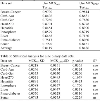
Table 4 shows the results from the experiment. From Table 4, we can see that the average testing accuracy obtained by MCSOARP is better than the
MCSAcc model. The average testing accuracy obtained
by MCSOARP model is 0.8439 while 0.8119 for the
MCSAcc model for all nine binary data sets. Overall, the
MCSOARP model shows an outstanding performance
against the MCSAcc model, whereby the MCSOARP
model has improved the classification performance in all binary data sets.
To verify this outstanding performance, we performed a paired t-test with 95% confidence level on each binary data set by using ten trial records for each data set. The summary result of this t-test analysis is listed in Table 5. As indicated in Table 5, the MCSOARP
model obtained six significant wins, while the other three data sets show no significant differences between
Table 4: Average testing accuracy for both MCS models.
Data set Use MCSAcc Use MCSOARP
TestAcc TestAcc
Breast-Cancer 0.9700 0.9814
Card-Aus 0.8406 0.8681 Card-Ger 0.7260 0.7630
Heart270 0.8704 0.8778
Hepatitis 0.8454 0.8900
Ionosphere 0.8579 0.8719
Liver 0.6468 0.7160
Pima-diabetes 0.7513 0.8060
Sonar 0.7990 0.8181
Average 0.8119 0.8436
Table 5: Statistical analysis for nine binary data sets.
Data set MCSAcc SD MCSOARP SD p-value S?
Breast-Cancer 0.0218 0.0151 0.0365 ssw
Card-Aus 0.0246 0.0364 0.0324 ssw
Card-Ger 0.0375 0.0330 0.0260 ssw
Heart270 0.0531 0.0495 0.1679 ns
Hepatitis 0.0891 0.0671 0.0423 ssw
Ionosphere 0.0588 0.0357 0.1760 ns
Liver 0.0736 0.0447 0.0338 ssw
Pima-diabetes 0.0550 0.0328 0.0110 ssw
Sonar 0.0793 0.0575 0.2229 ns
Note: SSW: Statistically Significant Win; SSL: Statistically Significant Loss; NS: Not Significant
the MCSOARP and MCSAcc. On top of that, we also
performed a t-test analysis on the average testing accuracy obtained by both models over nine binary data sets (Table 4). From this analysis, the MCSOARP metric
shows a significant difference with the MCSAcc model
at confidence level of 95% and even 99% where p-value is 0.0021.
DISCUSSION
The experimental results have shown that the MCSOARP model has outstandingly outperformed if
compared to the MCSAcc model for all binary data sets
in terms of predictive accuracy. Empirically, we have proved that the OARP metric is more discriminating than the accuracy metric in selecting and discriminating the optimized solution for stochastic classification algorithm, which in turn produced a higher accuracy of predictive results. This somewhat against a common intuition in machine learning that a classification model should be optimized by a performance metric that it will be measured on. This finding is also consistent with reports from studies in (Huang and Ling, 2005; Rosset, 2004).
We believe that the OARP metric works effectively with the stochastic classification model in leading towards a better training model. In this particular paper, the MCS model optimized by the OARP metric was able to select and discriminate better solution as compared to its performance with the conventional accuracy metric alone. This indicates that the OARP metric is more likely to choose an optimal solution in order to build an optimized classifier for stochastic classification algorithm.
CONCLUSION
In this study, we proposed a new performance metric called the Optimized Accuracy with Recall-Precision (OARP) based on three existing metrics, which are the accuracy and the extended recall and precision metrics. Theoretically, we proved that our newly constructed performance metric satisfied the above criteria using four analysis examples with different types of class distribution. To support our theoretical evidence, we compared experimentally the new metric against the accuracy metric using nine real binary data sets. Interestingly, the MCS model optimized by the OARP metric has outperformed and statistically significant than the MCS model optimized by the accuracy metric. The new OARP metric is proven to be more discriminative, robust to the changes of class distribution and also favored the small class distribution.
For the future study, we are planning to extend this new performance metric, OARP for solving multi-class problems. Moreover, we are also interested to conduct an extensive comparison between the OARP metric against different performance metrics in optimizing the heuristic or stochastic classification models.
REFERENCES
Al-Bayati, A.Y.A., N.A. Sulaiman and G.W. Sadiq, 2009. A modified conjugate gradient formula for back propagation neural network algorithm. J. Comput. Sci., 5: 849-856. DOI: 10.3844/jcssp.2009.849.856
Al-Shalabi, L., Z. Shaaban and B. Kasasbeh, 2006. Data mining: A preprocessing engine. J. Comput. Sci., 2: 735-739. DOI:10.3844/jcssp.2006.735.739 Bezdek, J.C. and L.I. Kuncheva, 2001. Nearest
prototype classifier designs: An experimental study. Int. J. Intell. Syst., 16: 1445-1473. DOI: 10.1002/int.1068
Bradley, A.P., 1997. The use of the area under the ROC curve in the evaluation of machine learning algorithms. Patt. Recog., 30: 1145-1159. DOI: 10.1016/S0031-3203(96)00142-2
Caruana, R. and A. Niculescu-Mizil, 2004. Data mining in metric space: An empirical analysis of supervised learning performance criteria. Proceedings of the 10th ACM SIGKDD International Conference on Knowledge Discovery and Data Mining, (KDD’04), ACM, New York, NY, USA., pp: 69-78. DOI: 10.1145/1014052.1014063
Ferri, C., P.A. Falch and J. Hernandez-Orallo, 2002. Learning decision trees using the area under the ROC curve. Proceedings of the 19th International Conference on Machine Learning, (ICML’02), Morgan Kaufmann Publisher Inc., San Francisco, CA, USA, pp: 139-146.
Garcia-Pedrajas, N., J.A. Romero del Castillo and D. Ortiz-Boyer, 2010. A cooperative coevolutionary algorithm for instance selection for instance-based learning. Mach. Learn., 78: 381-420. DOI: 10.1007/s10994-009-5161-3
Huang, J. and C.X. Ling, 2005. Using AUC and accuracy in evaluating learning algorithms. IEEE Trans. Knowl. Data Eng., 17: 299-310. DOI: 10.1109/TKDE.2005.50
Kohonen, T., 2001. Self-Organizing Maps. 3rd Edn., Springer, USA., ISBN-10: 3540679219, pp: 521. Kononenko, I. and I. Bratko, 1991. Information-based
evaluation criterion for classifier’s performance. Mach. Learn., 6: 67-80. DOI: 10.1023/A:1022642017308
Lingras, P. and C.J. Butz, 2007. Precision and recall in rough support vector machines. Proceedings of the IEEE International Conference on Granular Computing, Nov. 2-4, IEEE Xplore, Halifax, pp: 654-654. DOI: 10.1109/GrC.2007.77
Pandya, A.S. and R.B. Macy, 1996. Pattern Recognition with Neural Networks in C++. 1st End., CRC Press, Inc., USA., ISBN0849394627, pp: 410. Provost, F. and P. Domingos, 2003. Tree induction for
probability-based ranking. Mach. Learn., 52: 199-215.
DOI: 10.1023/A:1024099825458
Ranawana, R. and V. Palade, 2006. Optimized precision - a new measure for classifier performance evaluation. Proceedings of the IEEE World Congress on Evolutionary Computation, (WCEC’06), IEEE Xplore, Vancouver, Canada, pp: 2254-2261. DOI: 10.1109/CEC.2006.1688586 Rosset, S., 2004. Model selection via the AUC.
Seliya, N., T.M. Khoshgoftaar and J. Van Hulse, 2009. Aggregating Performance Metrics for classifier Evaluation. Proceedings of the IEEE International Conference on Information Reuse and Integration, Aug. 10-12, IEEE Xplore, Las Vegas, Nevada, USA., pp: 35-40. DOI: 10.1109/IRI.2009.5211611 Skalak, D.B., 1994. Prototype and feature selection by
sampling and random mutation hill climbing algorithms. Proceedings of the International Conference on Machine Learning, (ICML’94), Morgan-Kaufmann, pp: 293-301.