THERMAL SCIENCE, Year 2012, Vol. 16, No. 1, pp. 53-67 53
NUMERICAL STUDY OF THE CONJUGATE HEAT TRANSFER IN
A HORIZONTAL PIPE HEATED BY JOULEAN EFFECT
by
Sofiane TOUAHRI and Toufik BOUFENDI*
Physic Energetic Laboratory, Department of Physic, Faculty of Sciences, Mentouri University, Constantine, Algeria
Original scientific paper DOI: 10.2298/TSCI101120080T
The 3-D mixed convection heat transfer in a electrically heated horizontal pipe conjugated to a thermal conduction through the entire solid thickness is investigated by taking into account the thermal dependence of the physical properties of the fluid and the outer heat losses. The model equations of continuity, momentum, and energy are numerically solved by the finite volume method. The pipe thickness, the Prandtl and the Reynolds numbers are fixed while the Grashof number is varied from 104 to 107 The results obtained show that the dynamic and thermal fields for mixed convection are qualitatively and quantitatively different from those of forced convection, and the local Nusselt number at the interface solid-fluid is not uniform: it has considerable axial and azimuthally variations. The effect of physical variables of the fluid depending on temperature is significant, which justifies its inclusion. The heat transfer is quantified by the local and average Nusselt numbers. We found that the average Nusselt number of solid-fluid interface of the duct increases with the increase of Grashof number. We have equally found out that the heat transfer is improved thanks to the consideration of the thermo dependence of the physical properties. We have tried modelling the average Nusselt number as a function of Richardson number. With the parameters used, the heat transfer is quantified by the correlation: NuA = 12.753 Ri
0.156 .
Key words: mixed convection, cylindrical pipe, conjugate heat transfer, finite volume method
Introduction
In the large domain of fluid thermal processes, the cylindrical horizontally pipe is a device that plays a major role in the transport of the working fluid and simultaneously in his heating or the cooling. The mixed convection heat transfer mode is a combination of the geometrical orientation and the heating of the pipe with an appropriate mass flow rate through it. Orfi et al. [1] investigated numerically the problem of bifurcation for fully developed laminar mixed convection of a Boussinesq fluid within inclined tubes subject to a uniform wall heat flux. Dual solutions characterized by two and four vortex secondary flow structure in a cross-section normal to the longitudinal axis of the tube have been found for different
combinations of the Grashof number and the inclination of the tube for all Prandtl numbers between 0.7 and 7.Numerical experiments carried out for developing flows indicate that the two-vortex solution is the only stable flow structure. Kokugan et al. [2] performed an experimental work in a heated vertical open tube at constant wall temperature.Correlations between the Grashof and the Reynolds numbers have been derived by setting up a mechanical energy balance in the tube. The results have been compared with available numerical results and showed good agreement. Fukusako et al. [3] investigated the influence of the inversion of the density and free convection heat transfer of air-water layers in a vertical tube with uniformly decreased wall temperature. Holographic interferometry was adopted to determine the time-dependent temperature distribution in the tube. The temperature, the flow patterns and the heat transfer characteristics along the tube wall have been determined. The simultaneously developing mixed convection, with constant physical properties, in an inclined heated pipe is considered in the numerical study of Ouzzane et al. [4], the authors studied four different cases: the pipe thickness is considered or neglected and in each case the heating is over the entire circumference or over the top half of it, the lower half being insulated. It is reported that neglecting the circumferential conduction within the pipe thickness leads to an overestimation of the azimuthally wall temperature difference, at a given pipe section. Extensive experimental data was provided by Mohammed et al. [5] on uniformly heated constant wall heat flux in a vertical circular pipe with different inlet configurations: cylindrical pipes with different length, sharp-edge, and bell-mouth. He showed that the inlet conditions and configurations have a tremendous effect on the heat transfer results. These same authors [6] have presented a numerical work with a computational model that has been successfully validated by comparing their experimental results [5] and other authors. Kurnia et al. [7] have carried out a parametric study of laminar flow and heat transfer characteristics of coils made of tube of several different cross-sections with the aim to conduct the geometrical effect on the heat transfer performance. The working fluid air and water are temperature-dependent. They found that in-plane spirals ducts give higher heat transfer rates. The azimuthally temperature variation at the outer surface of an electrically and uniformly heated inconel horizontal pipe is reported in the experimental study of Abid et al. [8]. The considered pipe is 1 m long having a 1 cm outer diameter and 0.02 cm thickness. The infrared thermal imaging measurements of the temperature at the pipe outer surface has shown a temperature difference between the top and bottom of the pipe that increases from 0 °C at the inlet of the pipe to 25 °C at the exit. In a previous work, the problem of conjugate heat transfer in a duct was numerically simulated by Boufendi et al. [9], under specific conditions chosen to allow the comparison with the experimental results of [8]. The obtained results with first order precision of the numerical schemes show a good agreement with the experimental values [8] and so validate the numerical code.
In this work, the problem of the 3-D conjugate, conduction in the wall and convection in the fluid, laminar mixed convection in a horizontal pipe with a small thickness heated by variable electric current is investigated thoroughly. In fact, this investigation is a logical continuation of the perspectives opened in the early results and detailed by
Boufendi [10]. The numerical methodofresolution used is a second order finite volume
THERMAL SCIENCE, Year 2012, Vol. 16, No. 1, pp. 53-67 55 properties on the heat transfer is also considered and the average Nusselt numbers obtained in this study are correlated with the Richardson numbers.
The mathematical model
We consider a long horizontal pipe having a length L = 1 m, an inside diameter Di = 0.96 cm and an external diameter Do = 1 cm (fig. 1). The pipe is made of Inconel having a thermal conductivity Ks = 20 W/mK. An electric current passing along the pipe (in the solid thickness) produced a heat genera-tion by the Joule effect. This heat is
transferred to distilled water flow in the pipe. At the entrance the flow is of Poiseuille type with an average axial velocity equal to 7.2·10–2 m/s and a constant temperature of 15 °C. The density is a linear function of temperature and the Boussinesq approximation is applied. The combined heat transfer in the solid and fluid domains is a conjugate heat transfer problem.
The physical principles involved in this problem are well modeled by the following non-dimensional conservation partial differential equations with their initial and boundary conditions:
* * * *
r *
At 0 : 0
0 :
t V V T
At t
(1)
– mass conservation equation
* *
* * r
* * * *
1 1
(r V ) V Vz 0
r r r z (2)
– radial momentum conservation equation
*2 *
* * * * * * *
r
r r r z r
* * * * * *
* *
*
* * * * *
0 θθ
rr r rz
* 2 * * * * *
0 0
1 1
( ) ( ) ( )
Gr 1 1 1
cos ( ) ( ) ( )
Re Re
V V
r V V V V V V
t r r r z r
P
T r
r r r r q r z (3)
– angular momentum conservation equation
* * *
* * * * * * * r
r z
* * * * * *
* *
* *2 * * *
0
r z
* 2 *2 * * *
0 0
1 1
( ) ( ) ( )
Gr
1 1 1 1
sin ( ) ( ) ( )
Re Re
V V V
r V V V V V V
t r r r z r
P
T r
r r r r z (4)
– axial momentum conservation equation
– energy conservation equation
The viscous stress tensor components are:
*
* *
* * r * * * * r
rr * r r * * *
* * * *
* * θ r * * * z
z z
* * * *
* * *
* * z * * * z r
zz * zr rz *
1 2 1 1 2 2 V V V r
r r r r
V V V V
r r z r
V V V
z
z r
(7)
The heat fluxes are:
* * * *
* * * * *
r * , * * and z *
T K T T
q K q q K
r r r z (8)
The boundary conditions
The previous differential equations are solved with the boundary conditions: – at the pipe entrance – z*= 0
– in the fluid domain – 0 £ r*£ 0.5 and 0 £q£ 2p
* * * * *2
r 0, z 2(1 4 )
V V T V r (9)
–in the solid domain – 0.5 £ r*£ 0.5208 and 0 £q£ 2p
* * * *
r z
0
V
V
V
T
(10)– at the pipe exit – z*= 104.17 *
* * * * * * *
z
r z z z z
* * * * *
*
* * * *
rz z zz
* * * * *
0
1 1
( ) ( ) ( )
1 1 1
( ) ( ) ( )
Re V
r V V V V V V
t r r r z
P
r
z r r r z (5)
* * * * * * * * r z * * * * * * * * * * r z * * * * 0 0 1 1 ( ) ( ) ( )
1 1 1
( ) ( ) ( )
Re Pr T
r V T V T V T
t r r r z
G r q q q
r r r z (6)
where
*
*
0 0
in the solid Re Pr
0 in the fluid S
THERMAL SCIENCE, Year 2012, Vol. 16, No. 1, pp. 53-67 57 – in the fluid domain – 0 £ r*£ 0.5 and 0 £q£ 2p
*
* * *
* r
* * * * * 0
z V
V V T
K
z z z z z (11)
–in the solid domain – 0.5 £ r*£ 0.5208 and 0 £q£ 2p *
* * * *
r z * * 0
T
V V V K
z z (12)
– at the outer wall – r* = 0.5208
The conductive heat flux is equal to the sum of the heat fluxes of the radiation and natural convection losses
– for 0 £q£ 2p and 0 £ z*£ 104.17
* * *
*
* c i *
* 0 0 ( ) r z r
V V V
h h D
T
K T
K r
(13)
– where
2 2
( )( )
r
h T T T T (14)
The emissivity of the outer wall e is arbitrarily chosen to 0.9. The convective local heat transfer coefficient hc is derived from the correlation of Churchill et al. [11] valid for all Prandtl and for Rayleigh numbers in the range of 10−6≤ Ra ≤ 109:
2 6 c i 8 air 9 16 27 air 0.387 Ra Nu 0.6 0.559 1 Pr h D K (15)
The Rayleigh and the Prandtl numbers are defined, respectively, as: 3
0 0 air
air
air air air
g [ ( , , ) ]
Ra T R z T D , Pr
v (16)
In this expressions of the Rayleigh and the Prandtl numbers the thermophysical properties of the air ambient are evaluated at the local film temperature given as: Tfilm = = [T(R0, q, z) + T]/2.
The Nusselt numbers
At the solid-fluid interface, the local Nusselt number is defined as:
*
* *
* *
* i 0.5
* * * *
0 b
( , ) Nu( , )
(0.5, , ) ( ) r
T K
r h z D
z
K T z T z (17)
The axial Nusselt number is defined as: 2π
* *
0
1
Nu( ) Nu( , )d
2
z z (18)
Finally, we can define an average Nusselt number for the whole solid-fluid interface:
2 104.17
* * A
0 0
1
Nu Nu( , )d d
2 104.17 z z (19)
The numerical method
For the numerical solution of modelling equations, we used the finite volume method well described by Patankar [12]; the sing of this method involves the discretization of the physical domain into a discrete domain constituted of finite volumes where the modelling equations are discretized in a typical volume. We used a temporal discretization with a truncation error of (Dt*)2 order. The convective and non-linear terms have been discretized
according to the Adams-Bashforth numerical scheme, with a truncation error of (Dt*)2 order,
the diffusive and pressure terms are implicit. Regarding the spatial discretization, we used the central differences pattern with a truncation error of (Dr*)2, (Dq*)2, and (Dz*)2 order. So our
spatio-temporal discretization is second order. The mesh used contains 52 × 88 × 162 points in the radial, azimuthal, and axial directions. In the radial direction, only 10 points are located in the small solid thickness. The considered time step is Dt* = 5·10–4 and the time marching is
THERMAL SCIENCE, Year 2012, Vol. 16, No. 1, pp. 53-67 59
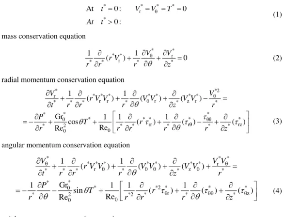
Figure 2. Axial evolution of the circumferentially mean axial Nusselt number; a comparison with the results of Ouzzane et al. [4]
Results and discussions
All the results presented in this paper were calculated for Reynolds number, Re = = 606.85, and the Prandtl number, Pr = 8.082, while the Grashof number is varied 104 ≤ Gr ≤
£ 107 (dependent with the volumetric heating). The obtained flow for the studied cases is
characterized by a main flow along the axial direction and a secondary flow influenced by the
density variation with temperature, which occurs in the plane r*−θ. Qualitatively we note the similarity of results for the seven studied cases. Quantitatively, the effect of mixed convection becomes increasingly important with the increase of volumetric heating.
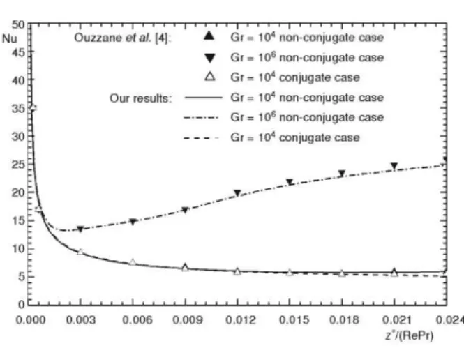
Development of the secondary flow
At the entrance z* = 0, the transverse flow is inexistent and the flow is axisymmetric. Just after the entrance, the generation of internal energy induced by the Joulean effect creates a radial thermal gradient oriented towards the inner fluid such as the hot fluid is close to the inner wall and the relatively colder fluid is in the core of the section. This situation induces necessarily a buoyancy force that raises the lighter fluid (the hotter fluid) towards the upper section (q = 0) of the duct and the heavier (colder fluid) towards the bottom (q = p) of the
section. This form of convective circulation of the fluid in the transverse plane of the section is called as secondary flow and appears as a two identical counter-rotating cells or vortexes in the plane r*−θ that each vortex circulates in one half section at opposed direction. The form and the position of the cells of the transverse flow are variant in axial direction. The vertical plane passing through the angles q = 0 and q = p is a plane of symmetry. This secondary flow
intensifies rapidly as illustrated by the values of the maximum angular component velocity and in fig. 3. For Gr = 104, the right hand maximum velocity of transversal flow V*max.= = 7.4470·10–3 located at z* = 104.17, r* = 0.4125,and q = 1.4993. For Gr = 105
, the velocity of secondary motion takes maximum value V*max. = 2.3420·10–
2
at z* = 34.8318, r* = 0.4125, and q = 1.4993. For Gr = 106, *
θ max
V 6.5540·10–2 at * 13.9978
z , r* = 0.4375, and q = 1.4993 and finally for Gr = 107, the secondary motion takes maximum velocity V*max.= 1.7790·10–
1
at z* = 11.3936, r* = 0.4625,and q = 1.4993.
the entrance and the station z* = 13.9978 where the centre of the right hand cell is located at r* = 0.3375 and q = 1.6422. Beyond this distance characterized by the development of secondary flow, there is a gradual decline to its established mode. At z* = 26.3680 the maximum velocity of transversal motion takes maximum value of V*max.= 6.0475·10–
2
at r* = 0.4625 and q = 1.7849, the center of the right hand cell in this section is located at r*
= 0.3875 and
q = 2.4989. Beyond this distance, the secondary flow remains almost invariant to the exit of the duct. At z*
= 104.17, the maximum V*max.= 3.7008·10– 2
is located at r* = 0.4375 and
q = 1.7850 .
Figure 3. Development of the secondary flow at selected axial positions for Gr = 106
Development of the axial flow
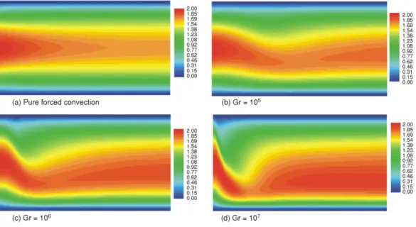
In the absence of heating volume (case of fluid flow without heat transfer) and in the case of forced convection (Gr* = 0) with a hydrodynamically developed flow at the entrance, the axial velocity exhibit concentric circular contours through all pipes and the flow field is axisymmetric. With the imposed Poiseuille’s flow at the entrance pipe, the axial velocity, at a given section, takes a maximum value at the pipe axis and a minimum value (0) at the internal wall of the pipe. In the presence of heating volume, the configuration of the flow changes automatically. The cylindrical symmetry is destroyed and the axial flow is influenced by the conjugate heat transfer between the wall and the fluid. The generated secondary flow affects the principal axial flow that is dependent on the temperature distribution within the pipe such as shown in figs. 4(a) and 4(d). We present in these figures the field of the non-dimensional axial velocities in the vertical plane passing through the angles q = 0 and q = p for four
THERMAL SCIENCE, Year 2012, Vol. 16, No. 1, pp. 53-67 61 increasing of heating volume, this effect takes a maximum value at z* = 34.8318, 13.9978, and 11.3936 for Gr = 105, 106, and 107, respectively.
Figure 4. Development of the axial velocity (color image see on our web site)
For a better explication of the development of the axial flow, we have chosen to represent in fig. 5 the axial velocity contours at selected axial sections (z* = 0.9766, 13.9978, L*/4, L*/2, 3L*/4, and L*) for the case Gr = 106. At the entrance, the flow is of Poiseuille’s type and the non-dimensional axial velocity takes a maximum value of Vz*max.= 2.0 at the pipe axis. Between the entrance and z* = 13.9978, the maximum axial velocity *
max. z
V changes a position rapidly towards the bottom of the pipe along the vertical diameter plane. This shifting is the result of the effect of a secondary motion. At z* = 13.9978, *
max. z
V = 1.9720 is located at r* = = 0.1768 and θ = π. Between z* = 13.9978 and z* = L*
/4, the value of Vz*max.decrease compared with the entrance region. At z* = 25.0659 (L*
/4), Vz*max. = 1.776 located at r* = = 0.3175 and θ = π. At z*
= 52.4105, Vz*max.= 1.8560located at r = 0.1768 and θ = π. Between z* = 77.8020 and z*
= 104.17, the value and position of Vz*max. is invariant and equal to 1.8820 at r* = 0.1280and θ = π.
Development of the temperature field
In the reference case (forced convection), the thermal field is axisymmetric and the isotherms, at given section, are concentric circles with a maximum temperature on the pipe wall and a minimum at pipe axis (r*= 0). In the presence of volumetric heating, a transverse flow exists and thus changes the axisymmetric distribution of fluid and pipe wall temperature and gives it an angular variation, this variation explained as follows: the hot fluid near the pipe wall moves upwards under the buoyancy force effect, the relatively cold fluid descends down in the middle of the pipe. This movement of the secondary flow is the cause of the azimuthally temperature variation. To illustrate the development of thermal field, we show in fig. 6, the polar temperature distribution at selected axial positions for Gr = 106. The obtained results
THERMAL SCIENCE, Year 2012, Vol. 16, No. 1, pp. 53-67 63 show that at given section, the maximum temperature T * is all the time located at r* = 0.5 and θ = 0 (top of solid-fluid interface), because the hot fluid is driven by the secondary motion towards the top of the pipe. The minimum temperature is within the core fluid, in the lower part of the pipe at θ= π. At the entrance, the fluid has a uniform temperature; far from the entrance the transversal motion gives an azimuthally fluid temperature variation. Atz*= = 26.3680 the minimum section temperature is located at r*= 0.3231. This position shifts to r*= 0.3719 and r*= 0.3841 at z* = 52.4105 and z* = 78.4530, respectively. We noticed that between z* = 78.4530 and z* = 104.17
the position of minimum temperature is invariant.
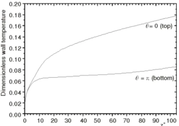
In fig. 7 we present the axial varia-tion of the dimensionless temperatures of the top (θ = 0) and the bottom (θ = π) of external wall (r* = 0.5208) for Gr = = 107. At z*=0, the temperature of the wall is uniform. After, the difference of temperature between the top and the bottom of the wall became important. At z* = 104.17, the external top and bottom walls take maximum tempera-ture values equal to T* = 0.1785 and 0.0865, respectively.
Development of the fluid physical properties
To show the significant change in physical properties with temperature, we present in fig. 8 the variation of dimensionless fluid dynamic viscosity for Gr = 107. At the entrance, the fluid temperature is 15 °C, The non-dimensional dynamic viscosity m* = m/m
0 = 1. At a given section, the viscosity is low near from the pipe wall and increases towards the relatively cold fluid. It is also clear that, closer to the wall, along the angular direction, the viscosity decreases continuously from the top to
the bottom of the pipe.
At the pipe exit, the fluid temperature became more superior than 15 °C, in this case m
*
takes a minimum value at the top of the pipe equal to 0.4 and maximum value equal to 0.94 at r* = 0.3275 and
q = p. As regards the dimensionless
thermal conductivity of the fluid, its variation is less important than the vis-cosity, it varies for the case of Gr = 5·105 from 1.001 at the entrance and 1.109 at the top of the pipe exit.
The comparison between results ob-tained by variable fluid properties and those obtained by constant fluid proper-ties show that the effect of secondary
Figure 7.Axial variation of the outer wall temperature forGr= 107 at the top and the bottom of the duct
Figure 8. The dimensionless dynamic viscosity variation for Gr = 5·105
flow is less important in the case of constant fluid properties, so the maximum azimuthally velocity *
max
V
is low in this case. The difference of temperature between the top and the bottom of the pipe wall decreases if the fluid properties are constant. The axial and average Nusselt numbers are more superior in the case of variable properties. These results are explained as follows: if the fluid proper-ties are constant the non-dimensional dynamic viscosity is equal to m* = 1in all fluid domain, the buoyancy force is reduced and the forced convection becomes relatively superior to natural convection, so we have a decrease in heat transfer. In fig. 9, we compare the results of axial Nusselt number obtained by the variable fluid properties and those obtained by constant fluid properties.It is clear that for each case, the axial Nusselt number obtained by variable fluid properties is more superior to that obtained by constant fluid properties. For Gr = 105, except at the entrance region, Nu(z) takes a maximum value equal to 10.9949 at the pipe exit for the case of variable fluid properties and 9.0853 for the case of constant fluid properties. For Gr = 106, at the pipe exit, Nu(z) = 18.7377 for the case of variable fluid properties, and 15.2243 for the case of constant fluid properties; finally, for Gr = 107, at the pipe exit, Nu(z) = 28.1002 for the case of variable fluid properties and 23.6073 for the case of constant fluid properties.
The average Nusselt number obtained by variable fluid properties for Gr = 105, 106, and107are: 10.121, 14.932, and 21.478, respectively, in the case of constant fluid properties, these values become 8.974, 13.165, and 19.428, respectively.
Heat transfer
The phenomenon of heat transfer has been characterised in terms of circumferentially Nusselt numbers calculated at the inner wall of the pipe, which is obtained by eq. (17). The variation of local Nusselt number of the solid-fluid interface is presented in fig. 10 for Gr = 107. From the entrance to the exit, we notice the large axial and angular variations of local Nusselt numbers, there is a monotonic axial increase of this latter which is characteristic of the enhanced heat transfer by the continuous mixing effect of the transverse flow, for each given section the local Nusselt number takes a minimum value at q = 0 and a maximum value at q = p.
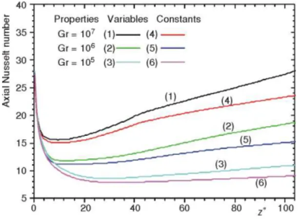
The axial Nusselt number Nu(z*) is obtained by eq. (18). Figure 11 shows the axial variation of Nusselt number for the eight studied cases. At the zone of entrance, the axial Nusselt number decreases rapidly for all studied cases. After, it increases and takes maximum value at the pipe exit equal to: 5.81, 6.54, 9.15, 10.99, 15.77, 18.74, 24.33 and 28.10 for Gr = = 0, 104 , 5·104, 105, 5·105, 106, 5·106, and 107,respectively. The axial Nusselt numbers increases with the increase of volumetric heating.
THERMAL SCIENCE, Year 2012, Vol. 16, No. 1, pp. 53-67 65
The average Nusselt number NuA is obtained by eq. (19). In tab. 1 we present the average Nusselt numbers of all studied cases.
Table 1. Average Nusselt numbers
Gr 104 5 × 10⁴ 105 5 × 10⁵ 106 5 × 10⁶ 107
Ri 0.027 0.136 0.272 1.358 2.715 13.577 27.154
NuA 7.960 9.114 10.121 13.128 14.932 19.112 21.478
The results obtained allowed us to model the average Nusselt number of the mixed convection in function of Richardson number, for this we used “ZunZun.com Online Curve Fitting and Surface Fitting Web Site” and
we found that the results with the parameters used are correlated with the correlation:
The fitting target of sum of squared absolute error is equal to: 7.065·10–1. In fig. 12 we present the fitting correlation. For each Richardson number between 0 and 28 we can obtain directly the average Nusselt number.
Conclusions
This study considers the numerical simulation of the 3-D mixed convection heat transfer in a horizontal pipe heated by an electrical intensity passing through its small thickness. The obtained results show that the dynamic and thermal fields for mixed Figure 10. The local Nusselt number variation for
Gr = 107 (color image see on our web site)
Figure 11. The axial Nusselt number variation for different Grashof numbers
Figure 12. The fitting correlation NuA = 12.753 Ri
0.156
convection are qualitatively and quantitatively different from those of forced convection. Although the volumetric heat input in the solid thickness is constant, the heat flux at the solid-fluid interface is not constant: it varies with q and z that is a characteristic of the considered mixed convection. The azimuthally variation of temperature at a given section is important; this phenomenon is demonstrated by the circumferential temperature variation of the wall: there is a large temperature wall difference between top and bottom of the external pipe. The comparison between the results obtained for the case of the physical constant properties and the case of the physical variable properties has showed that the Nusselt number is higher in the latter case. For the forced convection, the average Nusselt number is 7.775. Thus, for the mixed convection, the parameters used are well correlated with the correlation NuA = 12.753 Ri0.156.
Nomenclature
D – pipe diameter, [m]
G – volumetric heat generation, [Wm–3]
G* –
non-dimensional volumetric heat
– generation *
0 0
( Ks/ Re Pr ) ,[–]
Gr* – modified Grashof number (= gbG 5 2
/ s ) , i K D
– [–]
g – gravitational acceleration, (= 9.81), [ms–2]
h(q, z) – local heat transfer coefficient, [Wm–2K–1]
hc, hr – convective and radiative local heat transfer – coefficients respectively, [Wm–2K–1]
K – fluid thermal conductivity, [Wm–1K–1]
K* –
non-dimensional thermal conductivity,
– (K/K0), [–] *
s
K – non-dimensional solid thermal conductivity,
– (Ks/K0), [–]
L – pipe length, [m]
L* – non-dimensional pipe length (= L/D i), – [–]
NuA – average Nusselt number, [–]
Nu(z) – axial Nusselt number [= h(q,z)Di/K0], [–]
Nu(q, z) – local Nusselt number [= h(q, z)Di/K0], [–]
P – pressure, [Nm–2]
P* – non-dimensional pressure – [= (P–P0)/r0V02), [–]
Pr – Prandtl number (= n/a), [–] q – heat flux, [Wm–2 ]
r – radial co-ordinate, [m] *
r – non-dimensional radial co-ordinate (= r/Di), – [–]
R – pipe radius, [m]
Re – Reynolds number (= V0Di/v0), [–]
Ri – Richardson number (= Gr*/ 2 0
Re ), [–] T – temperature, [K]
T* –
non-dimensional temperature
– [= (T–T0)/(GDi2/Ks)], [–]
* b
T – non-dimensional mixing cup section
– temperature, [= (Tb–T0)/(GDi2/Ks)], [–]
t – time, [s]
t* – non-dimensional time (= V0t/Di), [–]
V0 – mean axial velocity at the pipe entrance, – [ms–1]
Vr, Vq, Vz – radial, circumferential and
– axial velocities components, – respectively, [ms–1]
* * *
r, θ, z
V V V – non-dimensional velocities
– components, (= Vr/V0, Vq/,V0, Vz/V0), – [–]
Z – axial co-ordinate, [m]
z* – non-dimensional axial coordinate, (= z/D i), – [–]
Greek symbols
a – thermal diffusivity, [m2s–1 ] b – thermal expansion coefficient, [K–1]
e – emissivity coefficient , [–]
q – angular co-ordinate, [rad]
m – dynamic viscosity, [kgms–1] *
μ – non-dimensional dynamic viscosity
– (= m/m0), [–]
n – kinematic viscosity, [m2s–1 ]
r – density, [kgm–3]
s – the Stephan-Boltzmann constant
– (= 5.67·10–8 ), [Wm–2K–4]
t – stress, [Nm–2]
*
τ – non-dimensional stress [= t/(m0/V0/Di)], [–] Subscripts
A – mean value b – bulk
i, o – reference to the inner and outer walls
– of the pipe
r, , z – reference to the radial, tangential, and axial
– directions, respectively s – reference to the solid
– reference to the ambient air away from
– the outer wall 0 – at pipe entrance
Superscript
THERMAL SCIENCE, Year 2012, Vol. 16, No. 1, pp. 53-67 67 References
[1] Orfi, J., Galanis, N., Bifurcation in Steady Laminar Mixed Convection Flow in Uniformly Heated Inclined Tubes, International Journal of Numerical Methods for Heat and Fluid Flow, 9 (1999), 5, pp. 543-567
[2] Kokugan, T., Kinoshita, T., Natural Convection Flow Rate in a Heated Vertical Tube, Journal of Chemical Engineering of Japanese, 8 (1975), 6, pp. 445-450
[3] Fukusako, S., Takahashi, M., Free Convection Heat Transfer of Air-Water Layers in a Horizontal Cooled Circular Tube, International Journal of Heat and Mass Transfer, 34 (1991), 3, pp. 693-702 [4] Ouzzane, M., Galanis, N., Effects of Parietal Conduction and Heat Flux Repartition on Mixed
Convection near the Entrance of an Inclined Duct (in French), International Journal of Thermal Sciences, 38, (1999), 7, pp. 622-633
[5] Mohammed, H. A., Salman Y. K., Laminar Air Flow Free Convective Heat Transfer Inside a Vertical Circular Pipe with Different Inlet Configurations, Thermal Science,11,(2007), 1, pp. 43-63
[6] Mohammed, H. A., Salman Y. K., Numerical Study of Combined Convection Heat Transfer for Thermally Developing upward Flow in a Vertical Cylinder, Thermal Science,12 (2008), 2, pp. 89-102 [7] Curnia, J. C., Sasmito, A., Mujumdar, A. S., Laminar Convective Heat Transfer for In-Plane Spiral
Coils of Non-Circular Cross-Sections Ducts, A Computational Fluid Dynamics Study, Thermal Science, 16 (2012), 1, pp. 109-118
[8] Abid, C., et al., Study of Mixed Convection in a Horizontal Cylinder. Analytic/Numeric Approach and Experimental Determination of Wall Temperature by Infrared Thermography (in French), International Journal of Heat and Mass Transfer, 37, (1999), 1, pp. 91-101
[9] Boufendi, T., Afrid, M., Three-Dimensional Conjugate Conduction-Mixed Convection with Variable Fluid Properties in a Heated Horizontal Pipe, Revue des Energies Renouvelables, 8, (2005), 1, pp.1-18 [10] Boufendi, T., Contribution to the Theoretical Study of Heat Transfer in a Horizontal Cylindrical Duct
Subjected to Mixed Convection Phenomenon (in French), Ph. D. thesis, University of Mentouri, Constantine, Algeria, 2005
[11] Churchill, S. W., Chu, H. S., Correlating Equation for Laminar and Turbulent Free Convection from a Horizontal Cylinder, International Journal of Heat and Mass Transfer, 18 (1975), 9, pp. 1049-1053 [12] Patankar, S. V., Numerical Heat Transfer and Fluid Flow, McGraw-Hill, New York, USA, 1980