Numerical simulation and decomposition of kinetic energy in the Central Mediterranean: insight on mesoscale circulation and energy conversion

www.ocean-sci.net/7/503/2011/ doi:10.5194/os-7-503-2011

© Author(s) 2011. CC Attribution 3.0 License.

Ocean Science

Numerical simulation and decomposition of kinetic energy in the

Central Mediterranean: insight on mesoscale circulation and

energy conversion

R. Sorgente1, A. Olita1, P. Oddo2, L. Fazioli1, and A. Ribotti1

1_{IAMC, Istituto per l’Ambiente Marino Costiero – Consiglio Nazionale delle Ricerche, Oristano, Italy} 2_{INGV, Istituto Nazionale di Geofisica e Vulcanologia, Bologna, Italy}

Received: 30 March 2011 – Published in Ocean Sci. Discuss.: 24 May 2011 Revised: 28 July 2011 – Accepted: 10 August 2011 – Published: 22 August 2011

Abstract. The spatial and temporal variability of eddy and mean kinetic energy of the Central Mediterranean region has been investigated, from January 2008 to December 2010, by mean of a numerical simulation mainly to quantify the mesoscale dynamics and their relationships with physical forcing. In order to understand the energy redistribution pro-cesses, the baroclinic energy conversion has been analysed, suggesting hypotheses about the drivers of the mesoscale activity in this area. The ocean model used is based on the Princeton Ocean Model implemented at 1/32◦ horizon-tal resolution. Surface momentum and buoyancy fluxes are interactively computed by mean of standard bulk formu-lae using predicted model Sea Surface Temperature and at-mospheric variables provided by the European Centre for Medium Range Weather Forecast operational analyses. At its lateral boundaries the model is one-way nested within the Mediterranean Forecasting System operational products.

The model domain has been subdivided in four sub-regions: Sardinia channel and southern Tyrrhenian Sea, Sicily channel, eastern Tunisian shelf and Libyan Sea. Tem-poral evolution of eddy and mean kinetic energy has been analysed, on each of the four sub-regions, showing different behaviours. On annual scales and within the first 5 m depth, the eddy kinetic energy represents approximately the 60 % of the total kinetic energy over the whole domain, confirming the strong mesoscale nature of the surface current flows in this area. The analyses show that the model well reproduces the path and the temporal behaviour of the main known sub-basin circulation features. New mesoscale structures have been also identified, from numerical results and direct obser-vations, for the first time as the Pantelleria Vortex and the Medina Gyre.

Correspondence to:R. Sorgente ([email protected])

The classical kinetic energy decomposition (eddy and mean) allowed to depict and to quantify the permanent and fluctuating parts of the circulation in the region, and to dif-ferentiate the four sub-regions as function of relative and ab-solute strength of the mesoscale activity. Furthermore the Baroclinic Energy Conversion term shows that in the Sar-dinia Channel the mesoscale activity, due to baroclinic insta-bilities, is significantly larger than in the other sub-regions, while a negative sign of the energy conversion, meaning a transfer of energy from the Eddy Kinetic Energy to the Eddy Available Potential Energy, has been recorded only for the surface layers of the Sicily Channel during summer.

1 Introduction

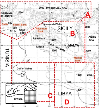
The Central Mediterranean region (CMED, hereafter), as previously defined by several authors (e.g. Astraldi et al., 1999; Ciappa, 2009), is a large area connecting the eastern and the western Mediterranean sub-basins. It is delimited by the eastern Sardinia Channel, the southern Tyrrhenian Sea and, mainly, the shallow (∼400 m) Sicily Channel (Fig. 1), an intermediate basin with an average depth of 500 m. It plays a crucial role in modulating the passage of the sur-face and intermediate water masses between the two Mediter-ranean sub-basins.

A

B

C

D

T

U

N

ISI

A

LIBYA

SICILY

Skerki Bank

Adventure Bank

Medina Bank

Pantelleria

MALTA

SIC_ILY CH_AN

NEL

TYRRHENIAN SEA

SARDINIA CHANNEL

IONIAN SEA

Galite

Gulf of Gabes

200 200

500

500

1000

1000

2000

2000

3000 3000

2000 1500

Linosa Cape

Bon

Mazara del Vallo

AFRICA

SPA IN

Fig. 1. The Central Mediterranean model bathymetry from US Navy DBDB1 (1/60◦). The boxes define the sub-domains where diagnostics are calculated: Sardinia Channel and southern Tyrrhe-nian Sea (box A), Sicily Channel (box B), Tunisian shelf area (box C) and Libyan area (box D).

continental shelves are very wide and cover more than one-third of the spatial extent of the Sicily Channel. In the Gulf of Gabes, the bathymetry is shallower than 30 m for large stretches away from the coast.

The circulation in the CMED is characterized by a number of significant dynamical processes covering the full spectrum of temporal and spatial scales (Millot, 1999; Pinardi et al., 1997). The surface and subsurface flows are mainly driven by the large scale Mediterranean thermohaline circulation, and clearly by the momentum and buoyancy fluxes at the air-sea interface. In addition there are wind-driven currents on the shelf due to remote storms; upwelling events off Sicily; sub-basin scale cyclonic and anticyclonic permanent gyres and small energetic mesoscale eddies with time scale shorter than 10 days (Manzella et al., 1988). The mesoscale struc-tures under the influence of wind stress, topography and in-ternal dynamical processes generate boundary currents and jets which can bifurcate, meander and grow then forming ring vortices and filament patterns interacting with the large scale flow fields (Lermusiaux, 1999; Lermusiaux and Robin-son, 2001).

The high variability of the water masses properties and cir-culation characteristics has been largely investigated in the past years through hydrographical observations (Manzella and La Violette, 1990; Sammari et al., 1999), sub-surface currentmeters data (Astraldi et al., 1999; Vetrano et al., 2004;

Gasparini et al., 2005), Lagrangian drifters (Poulain and Zambianchi, 2007) and high resolution numerical simula-tions (Onken et al., 2003; Sorgente et al., 2003; B´eranger et al., 2005). However, available observations are often char-acterized by poor spatial and temporal coverages, and are usually confined to the Italian seas while there is lack of ob-servations over the Tunisian and Libyan continental shelves. Only few datasets have adequate temporal and spatial resolu-tion to capture the mesoscale in local areas (Lermusiaux and Robinson, 2001).

Thus, numerical model simulations constitute an impor-tant tool to fill the observational gaps and to study the spa-tial and temporal ocean circulation variability. High resolu-tion models, below 5 km, were uncommonly used in the past mainly due to computational constraints. The computational issue poses the need to nest a hierarchy of successively em-bedded model domains, to downscale the large scale features to the coastal areas (Pinardi et al., 2003; Sorgente et al., 2003; Oddo et al., 2005). This methodology is found to be compu-tationally efficient and sufficiently accurate to transmit infor-mation across the connecting lateral open boundaries without excessive distortion (Oddo and Pinardi, 2008).

The aim of this study is to investigate the mesoscale and the sub-basin scale dynamics in the CMED region, by mean of decomposition of the simulated flow fields into mean and eddy components, then giving an overall assessment of the spatial and temporal mesoscale variability in relation with at-mospheric forcing and energy redistribution processes. The interest on mesoscale dynamic derives from the fact that eddies can potentially interact with the mean current and the bottom topography producing long term responses in the ocean circulation (Fernandez et al., 2005). The work has been done in the framework of the European COastal sea OPerational observing and forecasting system integrated project (ECOOP) funded by the European Commision’s Sixth Framework Programme, which main aim was the con-struction of an European network of sea-forecasting systems, through the improvement (resolution, physics, data assimila-tion, distribuassimila-tion, etc.) of existing operational models.

In order to improve the investigation of the dynamics in the area, the model domain has been subdivided in four sub-regions, each one supposedly characterized by an homoge-neous dynamics, as visible in Fig. 1: the Sardinia-Tyrrhenian area (area A); the Sicily Channel (area B); the wide and shal-low shelf area off Tunisia and Libya (area C); the wide slope area in front of Libya (area D).

2 The physical regimes

Three main spatial and temporal scales characterize the CMED: the large Mediterranean basin scale, including the thermohaline circulation; the sub-basin scale and the mesoscale. Each interacts with the others giving complex circulation patterns which arise from the multiple driving forces, strong topographic and coastal influences, and from internal dynamical processes (Robinson et al., 2001). 2.1 The large scale circulation

The main engine of the surface and subsurface large scale circulation is the remote forcing induced by the basin scale Mediterranean dynamics. The basin-scale thermohaline cir-culation in the Mediterranean Sea has been extensively stud-ied in the past years by several authors through observational programs and numerical modelling studies (Zavatarelli and Mellor, 1995; Pinardi et al., 1997; Pinardi and Masetti, 2000; B´eranger et al., 2005). The thermohaline circulation is anti-estuarine (lagoonal) and it is driven mainly by the balance between the relatively fresh waters entering at the Gibraltar Strait and the negative fresh-water budgets over the whole Mediterranean basin. This is usually described as a zonal cell which involves the exchanges of water masses between the eastern and the western Mediterranean sub-basins with the transformation of the surface Atlantic Water (AW) in the Levantine Intermediate Water. Thus, the vertical structure consists of a two-layer flow with the surface AW moving eastward from the Gibraltar Strait and spreading from the Sicily Channel throughout the eastern Mediterranean sub-basin as modified AW (Astraldi et al., 2002), and a salty Levantine outflow moving westward at intermediate depth. The zonal cell is connected with the “meridional” cells that are driven by the dense water mass formation processes oc-curring in the Gulf of Lions and Adriatic Sea (Schlitzer et al., 1991). In the Sicily Channel, the sill depth strongly mod-ulates the exchange of these deep and intermediate waters between the two Mediterranean sub-basins.

In the western Mediterranean sub-basin the amplitude of the seasonal variability is large and involves intense currents and mesoscale variability while, in the eastern sub-basin, the inter-annual and seasonal variabilities have the same order of magnitude involving the characteristics of the deep and intermediate water masses and high mesoscale activity (Ko-rres et al., 2000). Then, the CMED is a key area to mon-itor the thermohaline circulation and the corresponding hy-drological trends (Astraldi et al., 1999, 2002) of the entire Mediterranean Sea.

2.2 The sub-basin scale

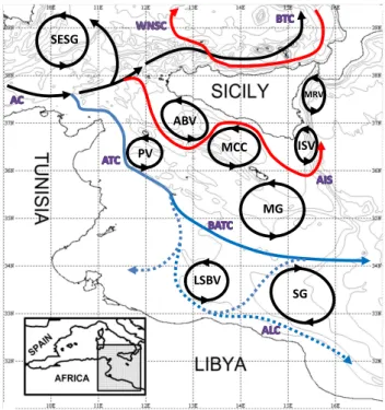
A schematic description of the seasonal variability of the sub-basin scale surface circulation, including the new features de-scribed in this paper, is represented in Fig. 2, as derived from

PV ABV

MCC ISV

MRV

SESG

MG

SG LSBV

Fig. 2. Schematic surface circulation with cyclonic/anti-cyclonic features (modified from Lermusiaux and Robinson, 2001; B´eranger et al., 2004 and Hamad et al., 2005) togheter with new features found in the present work. Acronyms are listed in Table 1. Perma-ment features/paths are in black while seasonal are in red (summer) and in blue (winter). Continuous lines are for features from bibli-ography while dotted are for new ones.

Lermusiaux and Robinson (2001); B´eranger et al. (2004) and Hamad et al. (2005). In the CMED the sub-basin scale fea-tures (jets, gyres and meanders) are part of the basin-wide circulation. The upper layer is occupied by the AW mov-ing eastward as Algerian Current (AC), a coastal boundary current whose instability generates meanders few kilometres long and coastal eddies (Robinson et al., 2001). The cyclonic eddies are relatively superficial and short-lived, while the an-ticyclones last for weeks or months (Sammari et al., 1999; Astraldi et al., 2002). These mesoscale phenomena are dis-turbed by the South Eastern Sardinia Gyre (SESG, hereafter), a sub-basin scale wind curl driven cyclonic gyre centred ap-proximately at 10◦E–38.5◦N (Artale et al., 1994) whose di-ameter varies between 200 and 300 km.

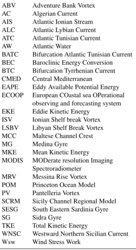
Table 1.Acronyms and abbreviations.

ABV Adventure Bank Vortex AC Algerian Current AIS Atlantic Ionian Stream ALC Atlantic Lybian Current ATC Atlantic Tunisian Current AW Atlantic Water

BATC Bifurcation Atlantic Tunisian Current BEC Baroclinic Energy Conversion BTC Bifurcation Tyrrhenian Current CMED Central Mediterranean

EAPE Eddy Available Potential Energy ECOOP European COastal sea OPerational

observing and forecasting system EKE Eddie Kinetic Energy

ISV Ionian Shelf break Vortex LSBV Libyan Shelf Break Vortex MCC Maltese Channel Crest MG Medina Gyre

MKE Mean Kinetic Energy MODIS MODerate resolution Imaging

Spectroradiometer MRV Messina Rise Vortex POM Princeton Ocean Model PV Pantelleria Vortex

SCRM Sicily Channel Regional Model SESG South Eastern Sardinia Gyre SG Sidra Gyre

TKE Total Kinetic Energy

WNSC Westward Northern Sicilian Current Wsw Wind Stress Work

salinity minimum: the Atlantic Tunisian Current (ATC) mov-ing over the Tunisian continental slope, and the Atlantic Io-nian Stream (AIS) along the southern coast of Sicily (As-traldi et al., 1996; Lermusiaux, 1999; Robinson et al., 1999; Lermusiaux and Robinson, 2001). It is worth to mention that the described bifurcation pattern is Gasparini et al. (2004) and by Gerin et al. (2009) from in situ data. They lightly dif-ferent from what estimated by Astraldi et al. (1999, 2002), found that AW directly splits in three veins at the entrance of the Sicily Channel following separate tracks with the minimum of salinity along Tunisia. Vice versa, during the 1994–1996 AIS investigation by Robinson et al. (1999), the ATC/AIS bifurcation has not been observed but only the AIS was present with southerly branches in the Sicily Channel and Ionian Sea in a complicated meandering path. These changes in currents and water mass properties confirm the strong temporal variability of the area, where the mesoscale activity can be considered as an important source of interan-nual variability (Fernandez et al., 2005).

The main stream associated to the ATC flows eastward along the Tunisian and Libyan continental shelf break just

south of Lampedusa or confined into the central part of the Sicily Channel (Manzella et al., 1988, 1990). The AIS con-stitutes a free jet energetic current mainly flowing eastward, along the southern coast of Sicily, as a typical waveform forcing upwelling on the Adventure Bank (western Sicil-ian shelf), especially during the summer when the current is strong. An important spatial variability exists and in-cludes: shape, position and strength of permanent or quasi-permanent sub-basin gyres and their unstable lobes, mean-ders patterns, bifurcation structures and strength of perma-nent jets, transient eddies and filaments (Robinson et al., 1999).

The sub-basin scale structures have seasonal amplitudes associated with the large wind stress variability (Pinardi and Navarra, 1993; Molcard et al., 2002). Recently, numerical studies (Onken et al., 2003; Sorgente et al., 2003; B´eranger et al., 2004) and direct observations (Astraldi et al., 1996; 1999; Sammari et al., 1999; Poulain and Zambianchi, 2007) have been devoted to assess the seasonal characteristics of the surface circulation. Superimposed to such seasonal (sub-basin) variability there is also a signal of interannual vari-ability mainly due to the mesoscale and, in some measures, to lower frequency signals related to climate change (Olita et al., 2007).

2.3 The mesoscale

Mesoscale variability can be defined as the ensemble of flow fluctuations whose periods range from a few days to a few tenths of days. Many events are included in this broad def-inition, among which we are mostly interested in mesoscale variability associated to small vortices (i.e. mesoscale ed-dies). Its forcing mechanisms are mainly instabilities of the large-scale circulation, interactions between currents and bathymetry and the direct surface forcing. The interest in the CMED mesoscale dynamics comes from the hypothesis that fronts, jets, meanders and eddies can play an important role in the ocean as response to buoyancy forcing, winds and topographic gradients.

The horizontal scale of mesoscale eddies is related to the first baroclinic Rossby radius of deformation which, in the Sicily Channel, varies seasonally ranging from a minimum of about 8 km in January, to about 11 km during the period of stratification (Borzelli and Ligi, 1998). The radius almost vanishes in winter, over the Tunisian and Libyan shelf shal-low area, due to a complete mixing of the water column.

(1999) and Lermusiaux and Robinson (2001) using a four-dimensional numerical primitive equation model and inten-sive in-situ data during August–September 1996, but lim-ited to northern Sicily Channel. All of them found that the main features of dominant mesoscale variability are asso-ciated with five features: Adventure Bank Vortex, Maltese Channel Crest, Ionian Shelf break Vortex, Messina Rise Vor-tex and temperature and salinity fronts of the Ionian slope with their meanders and topographic wave patterns.

3 Methods

3.1 Model design

In order to reach an adequate resolution to model the mesoscale dynamics in the CMED, a nesting approach has been adopted. The Sicily Channel sub-Regional Model (SCRM, hereafter) has been embedded into the coarse basin model of the Mediterranean Forecasting System (MFS1671, hereafter; Tonani et al., 2008). This permits to produce a more detailed description of the circulation in the region, including some mesoscale components that cannot be re-solved by the coarse model. SCRM is a free surface three-dimensional primitive equation finite difference hydrody-namic model based on the Princeton Ocean Model (Blum-berg and Mellor, 1987). It solves the equations of continuity, motion, conservation of temperature, salinity and assumes that the fluid is hydrostatic and the Boussinesq approxima-tion is valid. The density is calculated by an adaptaapproxima-tion of the UNESCO equation of state revised by Mellor (1991). The vertical mixing coefficients for momentum and tracers are calculated using the Mellor and Yamada (1982) turbulence closure scheme, while the horizontal viscosity terms are pro-vided by the Smagorinsky parameterization (Smagorinsky, 1993).

SCRM is implemented between 9◦E and 17.10◦E and from 31.50◦N to 39.50◦N with a horizontal resolution of 1/32◦(∼3.5 km). In the vertical it uses 30 sigma levels, with more coverage near the surface following a logarithmic dis-tribution. The external time step is set to 4 s, with an in-ternal every 120 s. The model bathymetry has been obtained from the US Navy Digital Bathymetric Data Base-DBDB1 at 1/60◦by bilinear interpolation into the model grid. The min-imum depth is set to 5 m. Additional smoothing is applied to reduce the sigma coordinate pressure gradient error (Mellor et al., 1994). The resulting model bathymetry is shown in Fig. 1.

The numerical system was run in free mode (i.e. without any data assimilation scheme) from January 2008 to Decem-ber 2010.

The model has been initialized at 00:00 on 1 January 2008 using dynamically balanced analyses fields from MFS1671 through an innovative tool based on the Variational Initializa-tion and Forcing Platform (Auclair et al., 2000). This method

is largely used in meteorological activities as drastically re-duces the amplitude of the numerical transient processes, generally following the initialization phases for several days after the initialization. This method has been proven to dras-tically reduce the spin up time of the SCRM slave 5-days forecasts by Gabers´ek et al. (2007) to some few hours. On the light of such a result it has been used in the present exper-imental setup, permitting to diminish the spin up time prob-lem.

Surface momentum and buoyancy fluxes are interactively computed by mean of dedicated bulk formulae developed and tested for the Mediterranean Sea in previous numerical exer-cises (Castellari et al., 1998; Tonani et al., 2008; Pinardi et al., 2003; Oddo et al., 2009). Fluxes computation takes into account model predicted sea surface temperature and the 6-h (00:00, 06:00, 12:00, 18:00 UTC) atmospheric parameters from European Centre for Medium range Weather Forecast operational analysis. The parameters are wind at 10 m a.s.l., air temperature at 2 m a.s.l., cloud cover, dew-point temper-ature and atmospheric pressure. These data have a horizon-tal resolution of 0.25◦_{and, successively, are mapped on the}

SCRM grid through bilinear interpolation and linearly inter-polated in time at each model time step.

The surface boundary condition for momentum is:

KM

∂u

∂z

z=η

= τ

ρ0

, (1)

whereτ is the wind stress vector,K_M is the vertical

kine-matic viscosity,ρ0= 1025 kg m−3is a reference density and

ηis the free surface elevation. The wind stress components use a drag coefficientCd=Cd(Ta,T,W) as function of the

wind amplitude (W), the air temperature (Ta) and the sea

sur-face temperature predicted by the model (T) following the polynomial approximation given by Hellerman and Rosen-stein (1983). The surface boundary conditions for potential temperature take the classic form:

KH

∂T ∂z

z=η

= QT

ρ0Cp

, (2)

whereQTis the net heat flux,Cp(4186 J kg−1 K−1)is the

specific heat capacity of pure water at constant pressure and

KHis the vertical heat diffusivity. The net heat flux (Eq. 2)

involves the balance between surface solar radiation (QS),

the net long-wave radiation (QB), the latent (QE)and

sen-sible (QH)heat fluxes. The heat flux components are

cal-culated using the formula by Reed (1977) for the short wave radiation flux and that by Bignami et al. (1995) for long wave radiation. The turbulent components (latent and sensible heat fluxes) are computed by mean of the bulk aerodynamic for-mulae proposed by Kondo (1975).

For the salinity flux we consider the water balance:

KH

∂S ∂z

z=η

C2=1σ (1)

H α

whereE=QE/LEis the evaporation rate interactively

calcu-lated,LE the latent heat of evaporation,P the monthly

pre-cipitation rate obtained from Legates and Willmott (1990),R

is the river runoff andSis the surface model salinity at the first level. In our simulations the runoffRis set to 0 because of the absence of rivers with significant discharge. The last term of Eq. (3) is the salinity flux correction and accounts for the imperfect knowledge ofE-P (P especially). S∗ is the monthly mean sea climatology surface salinity from Med6 dataset, that is based on the MEDATLAS dataset using the MODB (Mediterranean Oceanic Data Base) analyses tech-niques (Brasseur et al., 1996). 1σ (1)H is the thickness of the surface layer,αis the relaxation time andH the bottom depth. ValueC2is equal to 0.7 m day−1.

Lateral open boundary conditions are defined through a simple off-line one way nesting technique that represents an efficient way to downscale the model solutions from the basin-scale (∼7 km, the coarse model) to the sub-regional scale (∼3.5 km). It has been largely used in numerical weather predictions and recently in numerical oceanogra-phy to simulate the hydrodynamics of limited coastal ar-eas (Drago et al., 2003; Sorgente et al., 2003; Zavatarelli and Pinardi, 2003; Oddo and Pinardi, 2008). The SCRM is nested at the lateral open boundaries with MFS1671 cov-ering the whole Mediterranean Sea with a horizontal res-olution of 1/16◦ (Tonani et al., 2008; Oddo et al., 2009). The daily mean values of temperature, salinity, total velocity and elevation were transferred from the coarse spaced grid of MFS1671 to the finely spaced grid of the SCRM open boundaries through an off-line, one-way asynchronous nest-ing. The definition of the nested open boundary conditions is based on Sorgente et al. (2003).

3.2 Energy analysis

By taking in account previous experiences and in order to quantify the energy levels involved in the simulated circula-tion, in our work the flow field is divided into mean and eddy components. Generally, any velocity field (u,v,w) can be di-vided into a time independent component (U,V,W) and an eddy fluctuating part (time dependent,u′,v′,w′):

u=U+u′ v=V+v′ w=W+w′ (4) where the time independent part is obtained averaging tem-porally the full field over a given interval,m. For the three velocity components:

U= 1

m m

X

j=1

uj, V=

1

m m

X

j=1

vj W=

1

m m

X

j=1

wj. (5)

The m term indicates the temporal scale (annual or monthly, as defined into the Sect. 4.1 and 4.2),j–t his the daily mean field andu, v andw are the zonal, meridional

and vertical components of the total velocity respectively (as defined in Eq. 4).

The Total Kinetic Energy (TKE) per unit mass can be ex-pressed as:

TKE=1 2(u

2_+v2_),

substituting in the above equation the decomposition of the total velocity as defined in the Eq. (4), we obtain:

TKE=1 2(U

2_+V2₎₊1

2(u

′2_+v′2_{)+(U u}′

+V v′), (6) where the first term on the right hand side is the kinetic en-ergy of mean flow per unit mass (MKE):

MKE=1 2(U

2_+V2_{), (7)}

while the second term is the kinetic energy per unit mass of the fluctuating flow, also called Eddy Kinetic Energy (EKE): EKE=1

2(u

′2_+v′2_).

(8) The last term in the r.h.s of Eq. (6) is the first-order corre-lation term (Orlansky and Katzfey, 1991). The time average of TKE (Eq. 6) will contain only the first two terms (Eqs. 7 and 8), since the time mean of the third term vanishes. The logarithm of the ratio between the EKE (Eq. 8) and MKE (Eq. 7) defines the following parameter:

8=log(EKE

MKE) (9)

which provides information on the energy distribution be-tween the mean constant and fluctuating currents in the study area. In general, if8 < 0 then MKE prevails on EKE, if

8=0 then EKE and MKE are of the same order, otherwise if8 >0 then EKE is larger than MKE. This last condition suggests that the energy of currents is dominated by the ve-locity fluctuating component.

In order to evaluate part of the sources of energy for the mesoscale in the study area, the Baroclinic Energy Conver-sion (BEC) has been evaluated. BEC (Orlansky and Katzfey, 1991) is defined as:

BEC= −ρ′gw′ (10)

where g is the gravitational acceleration, w′ is the verti-cal component of the fluctuating velocity obtained applying Eq. (4), whileρ′ arises from the decomposition of the in-stantaneous densityρ(x,y,z,t )into a motionless part, a time independent component and a spatial and temporal varying component following the below equation:

ρ(x,y,z,t)=ρ(z)+ρ(x,y,z)+ρ′(x,y,z,t ).

We use the wind stress work to evaluate the relationship between TKE and the wind forcing. It is defined as:

W sw=u·τ (11)

whereuis the surface current vector andτ the wind stress

vector (Pedlosky, 1996; Zhai et al., 2007). The wind stress work (Wsw hereafter) represents the work done by the wind on the sea surface.

MKE and EKE have been vertically integrated and hor-izontally averaged over the four sub-regions previously de-fined and visible in Fig. 1 as follows:

ϑ (t )= 1

V

Z h2

h1

Z y2

y1

Z x2

x1

ϑ (x,y,z,t )dxdydz. (12) The integration limits are the coordinates delimiting the horizontal sub-domain (x andy) and the vertical layers (z), while the temporal scale (t) is defined into the Sect. 4.1 and 4.2. Moreover the grid point, whose depth of the first sigma layer exceeds 1 m, has been excluded (the deepest part of the Tyrrhenian Sea and of the east Ionian escarpment).

3.3 Data

In order to support results obtained by analyzing modelled fields, different sets of satellite measurements have been used.

Sea Level Anomaly data, used to support the observa-tions of relatively large and offshore mesoscale eddies, are AVISO SSALTO/DUACS mapped and gridded weekly prod-ucts with a spatial resolution of 1/8◦ (http://www.aviso. oceanobs.com/).

Ocean-Color 1 km data are Level-2 (single swaths) acquired from MODerate resolution Imaging Spectro-radiometer (MODIS) sensor on board of the AQUA mis-sion and downloaded from the oceancolor web portal (http: //oceancolor.gsfc.nasa.gov/). The Level-2 MODIS data have been post-processed and re-projected through SEADAS™ software.

4 Results and discussion

The spatial variability of MKE, EKE and the ratio of EKE over MKE (8) simulated by SCRM on the period 2008– 2010 are described on annual (Sect. 4.1) and monthly scale (Sect. 4.2), also comparing the simulated circulation with lit-erature. In Sect. 4.3, the temporal variability of BEC has been analyzed, giving information about the source of energy for mesoscale induced by baroclinic instabilities.

The MKE field has been computed as defined in the Eq. (7), while EKE was obtained according to Eq. (8). Suc-cessively, MKE and EKE have been vertically integrated over the first 5 m depth and horizontally averaged over the whole area and in the four sub-regions as previously defined (Eq. 12). We integrated our results over the upper 5 m depth,

Fig. 3. Maps of mean flow (panelA, [ms−1]), MKE (panel B, [cm2s−2]), EKE (panel C, [cm2s−2]) and the logarithmic ratio EKE over MKE (panelD) averaged on the period 2008–2010 and vertically integrated from surface to 5 m depth. In panel(A)the minimum velocity current represented is 5 cm s−1. In panels(B) and (C) areas with MKE and EKE larger than 100 cm2s−2 are shaded while the contour interval is 50 cm2s−2. In panel(D)the contour interval is 1.

that we consider representative for the surface layer. Our re-sults have been qualitatively compared with EKE estimates derived from the drifters-based work of Poulain and Zam-bianchi (2007), which is the only observational reference available for the area.

4.1 Mean circulation

The annual mean field of the simulated surface circulation is obtained by averaging the daily mean velocity fields of SCRM as described in Eq. (5) where m denotes the number of days over the simulated period (2008–2010). The model results are shown in Fig. 3, drawing the main characteris-tics of the basin and sub-basin mean surface circulation and confirming the results obtained from observations and pre-vious studies (e.g. Zavatarelli and Mellor, 1995; Robinson et al., 2001; Astraldi et al., 2001, 2002; Onken et al., 2003; B´eranger et al., 2004).

The AIS flows between Pantelleria and the southern Sicil-ian coast, then north of Malta and intrudes into the deep Ionian Sea after the overshooting along the eastern Sicilian coast, as described by Lermusiaux (1999) and Sorgente et al. (2003). High values of MKE (Fig. 3b) above 500 cm2s−2 are found over the Adventure Bank, along the southern Sicil-ian coast and along the IonSicil-ian shelf break. Apart the MKE patches over the Adventure Bank that could be overestimated because of an relatively smooth bathymetry, the simulated MKE distribution is generally in agreement with the paths detected by Poulain and Zambianchi (2007).

In the central part of the Sicily Channel the MKE appears rather weak. The ATC flows southward along the Tunisian coast as a relatively strong current decreasing progressively its velocity south-eastward. It flows approximately following the 200 m isobaths until Libya with MKE below 50 cm2s−2

between 12◦_{E and 14}◦_{E. This limited feature is also}

vis-ible in Fig. 3a and in full agreement with drifter observa-tions. We call this narrow current as Atlantic Libyan Current (ALC, hereafter) which can be considered as the eastward extension of ATC along the Libyan coast (Gasparini et al., 2008; Poulain and Zambianchi, 2007). A further dominant feature is the Sidra Gyre, previously mentioned by several authors (Korres et al., 2000; Sorgente et al., 2003; Fernan-dez et al., 2005; Tonani et al., 2008), a sub-basin permanent anti-cyclonic structure centred at about 33.5◦N and 16◦E and detected also by drifter trajectories (Poulain and Zam-bianchi, 2007). Its diameter is about 150–200 km. It strongly interacts with the ALC, pushing the modified AW toward the Libyan coast in a narrow stream. The Sidra Gyre appears as the main dynamical mechanism that influences the outflow of AW outside the Sicily Channel, having a seasonal and interannual variability, as stated by Gerin et al. (2009) and Ciappa (2009). It also controls the inflow of warm and salty Ionian Surface Water from the eastern side of the Libyan shelf through its southern arm. This feature is represented by a westward flow characterized by values of MKE of about 100 cm2s−2(Fig. 3b).

The EKE map (Fig. 3c), which includes the variability due to small scale eddies, to sporadic wind-driven current events and also to the seasonal modulation of the surface cir-culation with internal energy redistribution processes, shows almost the same spatial patterns observed for MKE, sug-gesting a strong variability associated to the intensity of the currents with larger values of TKE. Values of EKE less than 50 cm2s−2 _{are found at the deepest part of the Sicily}

Channel, below Malta. Vice-versa, large fluctuations over 100 cm2s−2_{are found in regions with strong currents, such}

as along the northern Tunisian shelf break (the AC), with the highest values (>350 cm2s−2)over the Skerki Bank, west-ward and along the northern Sicilian coast. This succession identifies the path of BTC, which does not clearly appear in the mean flow. Downstream the Sicily Channel, high values are found between Malta and Sicily and at significant topo-graphic gradients of the Ionian escarpment. Isolated

struc-tures also appear along the Libyan coast between 12◦_{E and}

14◦_{E. Most of them have been confirmed by the above}

men-tioned drifter observations, even if the model underestimates the energy content of these structures. This underestimate for MKE and EKE could be due to the different sampling periods, 1990–1999 for the drifter-based study and 2008– 2010 for the model, or to the unevenly sampling accom-plished through the drifters. Obviously, this disagreement in term of values could also be due to the other factors like the low resolution atmospheric forcing, an inadequate mod-elled viscosity-diffusivity or an insufficient vertical resolu-tion of the model. In any case our model results indicate that the mean EKE, averaged over the whole domain, is about 90 cm2s−2, three times MKE.

The energy ratio between the mean constant and fluctuat-ing currents is represented by the parameter8(Eq. 9) which compares the levels of MKE and EKE (Fig. 3d). The values with8 <0 identify the main stream currents where the mean flow kinetic energy is larger than EKE, as for AC and AIS. The areas where MKE and EKE are roughly similar (8=0) are identified by the paths of ATC with its bifurcations, ALC and the Sidra Gyre. Vice versa the EKE can be up about three times larger in logarithmic term than MKE (8 >1) into the deepest part of the Sardinia Channel and Tyrrhenian Sea, over the major part of the Tunisian shelf as isolated features in the Sicily Channel, between ATC and AIS, and between Malta and Libya westward of the Sidra Gyre where the mean flow is really weak.

4.2 Seasonal variability of kinetic energy and surface circulation

In order to analyze the MKE and EKE components of the ki-netic energy budgets, the simulated daily mean velocity fields of SCRM have been averaged on monthly basis over the pe-riod 2008–2010 computed as in Eq. (4) where m denotes the number of days for each month. The monthly averaged time series of TKE, MKE, EKE and the Wsw are shown in Fig. 4. The TKE (Fig. 4a), sum of MKE and EKE, has a seasonal cycle with values larger than 150 cm2s−2between Novem-ber and March. The EKE, always larger than MKE (Fig. 4b), dominates such a TKE seasonality following a similar cy-cle. Finally the MKE shows a smaller seasonal variability with an opposition phase period (EKE decreases while MKE increases) between May and July (relative maximum). The winter peaks of MKE and EKE appear to be related to the Wsw (Fig. 4c), which has values over about 0.3 N m−1_s−1

1 2 3 4 5 6 7 8 9 10 11 12 50

100 150 200

(A)

cm

2 s

−2

1 2 3 4 5 6 7 8 9 10 11 12 20

40 60 80 100 120

(B)

cm

2 s

−2

1 2 3 4 5 6 7 8 9 10 11 12 0

0.1 0.2 0.3 0.4 0.5

(C)

N m

−1

s

−1

Time (months)

Fig. 4. Time series of: monthly mean TKE (panelA, [cm2s−2]); MKE – solid line – and EKE – dashed line – (panelB, [cm2s−2]); Wsw (panelC, [N m−1s−1]). All time series has been averaged overall the model domain, vertically integrated from surface to 5 m depth and on the period 2008–2010.

The same analyses has been applied in each of the four sub-regions in which the whole domain has been divided (Fig. 1) in order to quantify possible differences in the spatial energy distribution and ratio (MKE, EKE and8).

4.2.1 The Sardinia-Tyrrhenian sub-region

The Sardinia-Tyrrhenian sub-region (A in Fig. 1) appears as the most energetic (Fig. 5). EKE is always larger than MKE apart in November and December. On an-nual mean the contribution of EKE to TKE is about 57 % on annual basis. The EKE shows a seasonal cycle with a maximum value in February (∼160 cm2s−2) and mini-mum in September (∼80 cm2s−2), while MKE shows val-ues over 100 cm2s−2 from November to January then pro-gressively decreasing towards its minimum values in April and September (∼60 cm2s−2) and a relative maximum in July (∼80 cm2s−2). The Wsw is characterized by two forc-ing regimes: from November to March it is always over 0.5 N m−1s−1, reaching its absolute maximum in December (0.8 N m−1_s−1_{), while from April to October it doesn’t}

ex-ceed 0.25 N m−1_s−1_{. Then the small MKE summer peak in}

July appears not directly related to the wind stress work. The comparison between EKE and MKE, represented by the pa-rameter8(see Eq. 9), shows a positive signal (8 >0) apart in November and December. This means that the surface dynamics is usually dominated by the velocity fluctuating component with its maximum in April (8∼0.8), while in November the mean flow on the velocity fluctuating compo-nent prevails (8 <0). We would underline the significance of such a ratio: the8parameter informs when/where EKE is

larger than MKE or, in other words, when mesoscale activity is stronger than the mean flow then neglecting the absolute value of EKE.

The horizontal distribution of 8in November (Fig. 6a) shows MKE prevailing on EKE (8 <0) in correspondence of AC and BTC paths. The mean flow of such features appear as coastal boundary currents flowing, respectively, along the northern Tunisian coast (AC) and along the northern Sicilian shelf break (BTC), in agreement with the literature (Astraldi et al., 1996; Molcard et al., 2002). Such a spatial feature is mainly due to the MKE field (not shown) reaching val-ues over 800 cm2s−2along the AC path that are compatible with speed currents of about 40 cm s−1then decreasing east-ward. Lower values (<200 cm2s−2)occur along the BTC path. The EKE is largely higher than MKE (8 >1), espe-cially in deep areas of the Sardinia Channel where the en-ergy of the currents is dominated by the fluctuating compo-nent, whose monthly mean reaches its maximum in February (Fig. 5b). The EKE field, with the current mean flow over-lapped, is represented in Fig. 6b. Values over 300 cm2s−2 are found along AC and BTC paths, increasing to the same order than MKE (not shown). Isolated patches of EKE show very high values (>400 cm2s−2) on the northern Tunisian shelf and along the northern Sicilian coast. EKE maxima are always associated with high energetic flows like the AC and BTC. BTC strength appears mainly related to the eastward flow at the Sardinia-Tunisia section (Fig. 7) and, secondly, to the atmospheric forcing (Fig. 5e). Vice-versa, the EKE pre-vails where there is not a clear mean flow, suggesting that the EKE signal would be due to instabilities generated along the currents boundaries.

Toward the summer months AC and BTC progressively decrease, in agreement with Astraldi et al. (2002) and Sor-gente et al. (2003), but the temporal evolution of MKE (Fig. 5c) shows a small increase on July. Here the model re-sults show the mean surface circulation dominated by the me-andering of a weaker AC, some split currents, cyclonic and anti-cyclonic eddies, the SESG and a westward coastal cur-rent flowing along the northern Sicilian coast (Fig. 8). SESG replaces part of the BTC path in summer and appears partic-ularly active in term of MKE from June to September (not shown). This coastal current seems to be part of a large anti-cyclonic gyre located on the southern side of the Tyrrhenian Sea. Actually there are no bibliographic indications on the existence of this feature which would deserve a more detailed study. We refer to this as Westward Northern Sicilian Current (WNSC, hereafter). It appears more stable and stronger than AC justifying the July increase of MKE described above. 4.2.2 The Sicily sub-region

1 2 3 4 5 6 7 8 9 10 11 12 0

50 100 150 200 250 300

(A)

TKE [cm

2 s −2]

Time (months)

1 2 3 4 5 6 7 8 9 10 11 12

0 20 40 60 80 100 120 140 160 180

(B)

EKE [cm

2 s −2]

Time (months)

1 2 3 4 5 6 7 8 9 10 11 12

0 20 40 60 80 100 120 140

(C)

MKE [cm

2 s −2]

Time (months)

1 2 3 4 5 6 7 8 9 10 11 12

−1 −0.5 0 0.5 1 1.5 2 2.5

(D)

Φ

=log(EKE/MKE)

Time (months)

1 2 3 4 5 6 7 8 9 10 11 12

0 0.1 0.2 0.3 0.4 0.5 0.6 0.7 0.8

0.9 (E)

Wsw [N m

−1 s −1]

Time (months)

Fig. 5. Time series of: TKE(A), EKE(B), MKE(C),8(D), Wsw(E); all time series have been averaged for the Sardinia-Tyrrhenian sub-region (continous-line, empty circle), Sicily sub-region (continuos-line, empty square), Tunisian sub-region (dashed-line, full square), Lybian sub-region (dashed-line, full triangle), vertically integrated from surface to 5m depth and on the period 2008–2010.

Fig. 6.Monthly mean map of Sardinia – Tyrrhenian sub-region for

8in November (panelA) and of the mean flow overlapped to EKE (panelB, [m s−1] and [cm2s−2] respectively) in February. Areas with EKE higher than 100 cm2s−2are shaded

1 2 3 4 5 6 7 8 9 10 11 12 1

2 3 4 5

Sv

Time (months)

Fig. 7. Monthly mean time series of the eastward flow [Sv] at the section Sardinia-Tunisia computed averaging the daily data from January 2008 to December 2010

Fig. 8.Monthly mean map for the Sardinia-Tyrrhenian sub-region of MKE [cm2s−2] in July averaged on the period 2008–2010 and vertically integrated from surface to 5 m depth. It puts in evidence the presence of the WNSC flowing along the northern Sicilian coast.

Fig. 9. December monthly map in the Sicily Channel sub-region for8(panelA), mean flow [m s−1] overlapped to EKE (panelB, [cm2s−2]) and MKE (panelC, [cm2s−2]) and streamlines of the mean flow (D, [m s−1]). Areas with MKE and EKE higher than 100 cm2s−2are shaded.

flow superimposed, is presented in (Fig. 9b). This figure shows the ATC as an offshore boundary current rather vari-able (EKE>150 cm2s−2)and intense, which progressively decreases southeastward along Tunisia. It is visible from Oc-tober to May and reaches its maximum intensity in December (not shown). Here the AIS is represented as a coastal current, less variable (EKE<100 cm2s−2_{)than ATC, flowing}

east-ward confined along the southern Sicilian coast in agreement with literature e.g. Ciappa (2009). In Fig. 9c high values of MKE (>800 cm2s−2)are isolated patches on the Adventure Bank, in correspondence of the Maltese Channel Crest and along the ATC path downstream Cape Bon. A contribution to the increase of the MKE along the ATC path is given by a small cyclonic vortex downstream the island of

Pantelle-Fig. 10. Panel(A): MODIS level-2 K490 image at 11 May 2009 where the Pantelleria Vortex is clearly defined south west of the Pantelleria island; panel(B): simulated surface velocity field for the same day where the depression corresponding to the vortex is clearly shown in the same position of the observation; panel(C): Sea Level Anomaly [m] map at 30 January 2009 where the Med-ina Gyre is evident as a wide depression (cyclonic) south of Malta; panel(D): the Medina Gyre at 1 February 2009 well identified in the simulated surface elevation [m].

ria (Fig. 9d) that constrains the core of the AW towards the Tunisian slope increasing its velocity. This mesoscale feature appears to be connected to ATC path and is located approx-imately at 11.75◦E–36.6◦N. We named this feature Pantel-leria Vortex (PV, hereafter). If particularly energetic, PV can induce a recirculation of AW into the Sicily Channel (not shown). Actually there are no bibliographic references on the existence of this feature from oceanographic surveys but PV is clearly identified by Ocean Color images (MODIS AQUA level 2 data). Figs. 10a and b show respectively MODIS K490 level 2 (reflectance at 490 nm wavelength, which is used in this case as passive tracer for dynamical features) and the simulated free surface elevation field at 11 May 2010 in the PV area. The PV is well identified and defined both in the simulated and observational satellite fields.

The monthly mean flow prevails on the velocity fluctuat-ing component in July (Fig. 5c) due to an increase of MKE, with a slight decrease of EKE (Fig. 5b), mainly induced by the AIS. Here the surface circulation (not shown) is repre-sented by an intense AIS which appears rather variable (EKE ∼100 cm2s−2_{). It reaches the largest values in the}

west-ern side of the Adventure Bank Vortex (MKE>800 cm2s−2₎

Fig. 11.Monthly mean map for the Tunisian sub-region in May of

8(panelA) and EKE (panelB, [cm2s−2], with mean flow [m s−1] superimposed) averaged on the period 2008–2010 and vertically integrated from surface to 5 m depth. Area with EKE larger than 60 cm2s−2are shaded.

1990) and numerical simulations (Sorgente et al., 2003; B´eranger et al., 2004).

4.2.3 The Tunisian – Libyan sub-region

The Tunisian–Libyan sub-region (C in Fig. 1) is a very shal-low area with maximum depths of about 250 m at its east-ernmost limit. Here the MKE is quite low while the monthly EKE values are up to four times higher than MKE (Fig. 5b, c) in logarithmic scale. The EKE contribution to TKE is there-fore dominant, reaching about 83 % on annual basis. This means that this area is almost completely controlled by the fluctuating currents. The wind stress (Fig. 5e) is very weak and does not seem to be the primary source of energy in this region. The EKE–MKE ratio (Fig. 5d) shows an absolute maximum in May and a relative maximum in October while the absolute minimum is in July.

The horizontal distribution of8for May (Fig. 11a) shows the whole sub-domain roughly dominated by the fluctuating component, with the highest ratio (8 > 3) between Libya and the 100 m isobath. This signal propagates northwest-ward, gradually decreasing. EKE and MKE are almost of the same order (8∼0) along the Libyan shelf break where the mean flow is represented by a weak current bounded by a cyclonic vortex approximately located at 12.8◦E–33.4◦N (Fig. 11b) that we call Libyan Shelf Break Vortex (LSBV in Fig. 2). LSBV appears as a permanent feature of the surface circulation from May to October whose position and strength contribute to frequent reversals of the coastal currents along the Libyan coast, together with the atmospheric forcing. This is shown by the high EKE values (>200 cm2s−2_)between

the southern side of the cyclonic vortex and the Libyan coast. Another interesting feature is represented by the western cur-rent coming from the center of the Sicily Channel towards the Gulf of Gabes. It appears weak (MKE<10 cm2s−2)and particularly evident in the model results from April to July under the forcing of easterly winds (not shown). This feature has been also observed by Poulain and Zambianchi (2007).

Fig. 12. Monthly mean map for the Libyan sub-region in October of8(panelA) and EKE (panelB, [cm2s−2]) superimposed on the mean flow [m s−1] averaged on the period 2008–2010 and vertically integrated from surface to 5 m depth. Area with EKE larger than 100 cm2s−2are shaded.

4.2.4 The Libyan sub-region

The Libyan sub-region (D in Fig. 1) has an important role in the thermohaline circulation of the Mediterranean Sea, as underlined by Gasparini et al. (2008). In this sub-region the contribution of EKE to TKE is about 65 % on annual ba-sis. The MKE and EKE signals are in phase without a clear seasonal cycle (Fig. 5). Their kinetic energies are found high through the whole year and particularly in June. It is difficult, even visually, to find any relation with the Wsw (Fig. 5e), which seems uncoupled from EKE. The Wsw is more intense than in the Tunisia – Libya sub-region and weaker than in the Sicily Channel and in the Sardinia – Tyrrhenian sub-region. The logarithm of EKE–MKE ratio (Fig. 5d) is always posi-tive (8 >0) with maximum values from August to October and minimum from March to June (8∼0.5).

Fig. 13. Monthly mean map of EKE superimposed on the mean flow [m s−1]in December over the Tunisian and Libyan areas.

circulation is the advection of warm and salty Ionian sur-face water, coming from the eastern side of the Libyan shelf, through a wide and weaker (MKE<120 cm2s−2) surface current flowing northwestward offshore Libya (not shown). The presence of this dense vein along the Libyan continen-tal margin has been also detected by Gasparini et al. (2008) during a cruise in 2006. The contrast between the Ionian sur-face water and the modified AW, advected by the ALC, can induce the formation of strong density gradients along the Libyan shelf break, as shown in the next section.

In this sub-region model results also show some unfamil-iar features like the splitting of ATC, approximately at 34◦_N

and 14◦_{E, that bifurcates in an eastward and a southward}

component (Fig. 13). The eastward current mainly flows into the Ionian Sea supported by the anti-cyclonic circula-tion (the Sidra Gyre). We named this branch as the Bifur-cation Atlantic Tunisian Current (BATC) represented by a wide, weak (MKE<150 cm2s−2) and stable surface current (EKE∼50 cm2s−2)particularly evident from November to April (not shown). Unfortunately the knowledge of the circu-lation in this area is rather poor due to a lack of observational data, as also recently underlined by Gasparini et al. (2008). Future investigations will be addressed to evaluate the favor-able conditions for the splitting of the ATC and on what in-fluences on its spatial and temporal variability.

4.3 Baroclinic Energy Conversion

The variability of the EKE of the circulation in the CMED has been depicted in the previous sections. In order to eval-uate and identify the part of the mesoscale activity due to baroclinic instabilities, the spatial and temporal variability of the BEC (Eq. 10) has been analyzed in the model domain and in each sub-region. The maps of BEC permit to represent the spatial distribution of the baroclinic instabilities at monthly scale.

1 2 3 4 5 6 7 8 9 10 11 12 −1

−0.5 0 0.5 1 1.5 2

J s

−1

m

−3 (*1e 4)

(A)

1 2 3 4 5 6 7 8 9 10 11 12 −2

0 2 4 6

J s

−1

m

−3 (*1e 4)

(B)

Time (month)

Fig. 14.Monthly time series of BEC for the Sardinia – Tyrrhenian (solid line and circle), Sicily Channel (solid line and empty square), Tunisian (dashed-dotted line and full squares) and Libyan (dashed line and triangles) sub-regions, as reported in Fig. 1, averaged on the period 2008–2010 and vertically integrated from the surface to 5 m depth (panelA) and from 5 to 80 m depth (panelB). Unit are Js−1m−3. The multiplication factor is 104.

Fig. 15. Monthly mean maps of BEC integrated from 5 to 80 m depth in February (panelA) and July (panelB), averaged on the period 2008–2010. Positive values indicate energy transfer from Eddy Available Potential Energy to EKE. Units are Js−1m−3. The multiplication factor is 104.

In the Sardinia – Tyrrhenian sub-region the BEC (Fig. 14b, solid line and circles) is almost two-three times larger than in the other sub-regions. Its temporal behaviour shows a large energy transfer from EAPE to EKE from November to March (>2e−5_{J s}−1_m−3_{), located over the fast flowing currents AC}

and BTC (Fig. 15a). This would be reasonably due to the density gradient generated between the inflow of modified AW through the Sardinia Channel (see Fig. 7) and resident water masses. From April to June the BEC is slightly positive while the inverse energy transfer mainly occurs in summer reaching its maximum in October. The BEC appears related to the correspondent EKE time series (Fig. 5b) and the in-flow of modified AW through the Sardinia Channel (Fig. 7). Then, in this area part of the mesoscale dynamics seems to be due to the energy conversion from EAPE to EKE, typical of baroclinic instability processes connected to the inflow of modified AW.

The Sicily Channel sub-region shows a slightly different trend in terms of energy conversion processes. The BEC sig-nal (see Fig. 14b, solid line and empty square) is character-ized by smaller values than those observed in the Sardinia Channel and by a positive seasonal cycle nearly through-out the year. The maximum energy transfer from EAPE to EKE occurs in February while we observe the inverse pro-cess in June. The BEC does not appear directly related to the EKE behaviour (see Fig. 5b). This is clearly evident if we consider the summer period when the EKE reaches its minimum in July and October. This weaker or null relation between the BEC and EKE suggests that, in the Sicily Chan-nel sub-region, the BEC is not the only source/loss of energy (Fig. 15b). In this area an important role would be played by the advective flows associated to the AIS, ATC and BATC, as well by the atmospheric forcing and the topographic con-strain.

Contributes to the domain averaged BEC in the Tunisian and Libyan sub-regions are always positive. This means that the energy conversion from EAPE to EKE occurs throughout the year at this layer. Highest levels of contribution to the baroclinic instability in the Tunisian sub-region mainly oc-cur from October to February (see Fig. 14b, dashed line and squares), well related to the EKE (see Fig. 5b). Differently the Libyan sub-region is the only sub-region where the en-ergy conversion reaches its maximum value in late summer (see Fig. 14b, dashed line and triangle), well related to the EKE time series (see Fig. 5b). Thus the internal energy redis-tribution processes reach their maximum in September when the work due to atmospheric forcing is almost at its lowest intensity (see Fig. 5e). This is associated with the inverse baroclinic energy conversion processes, where the EKE field motion restores the vertical and horizontal shears. In fact this region can accumulate EAPE during the winter then released to EKE during summer, when the BEC maxima are found above all in the Sicily Channel, along the southern Sicilian coast, due to the strong density gradient between the AIS and surrounding waters (Fig. 15b).

5 Conclusions

The circulation in the CMED has been simulated from Jan-uary 2008 to December 2010 using a high resolution primi-tive equations numerical model. The aim was to assess the spatial and temporal mesoscale variability and evaluate its relationships with the atmospheric forcing (winds) and the energy redistribution processes. So the simulated flow field has been decomposed into a mean and eddy (fluctuating) component that have been used to compute, respectively, the MKE (the kinetic energy of the mean flow) and the EKE (the kinetic energy of the fluctuating component); the latter as-sumed as a good indicator for mesoscale activity. Moreover, the spatial and temporal variability of the BEC has been anal-ysed in order to identify part of mesoscale activity due to baroclinic instabilities.

On the base of known oceanographic characteristics the model domain has been divided into 4 different sub-regions (Fig. 1): Sardinia-Tyrrhenian; Sicilian; Tunisian shelf; Libyan area.

The Sicily sub-region appears less energetic than the Sar-dinia – Tyrrhenian. MKE and EKE have almost comparable values without a clear seasonal cycle. The surface circula-tion is dominated by the seasonal modulacircula-tion between ATC (maximum in winter and fall) and AIS (in summer), by in-termittent eddy features, meanders and fronts which define the horizontal distribution of the surface waters. The foot-prints of the ATC in the MKE and the EKE fields indicate the ATC as a coastal boundary current, rather variable, flowing along the eastern Tunisian slope mainly from November to June in agreement with Sorgente et al. (2003) and B´eranger et al. (2004). The ATC is often accompanied by the PV, a small and intermittent mesoscale feature, induced by the potential vorticity stretching which can be involved on the recirculation of the AW into the Sicily Channel toward the Tunisian – Sicily section. During the summer months the ATC tends to vanish and it is replaced by a counter-current close to Cape Bon that is accompanied by a complex system of small cyclonic and anti-cyclonic eddies induced by baro-clinic instabilities. In the same months the MKE is sustained by the AIS which moves eastward with the typical waveform around permanent mesoscale features such as the Adventure Bank Vortex, the Maltese Channel Crest and the Ionian Shelf break Vortex (Robinson et al., 1999; Lermusiaux, 2001). In winter the AIS appears as a less intense coastal boundary cur-rent confined along the southern Sicilian coast, in agreement with satellite observations (Ciappa, 2009).

The Tunisian shelf sub-region appears characterized by strong mesoscale variability with an EKE two-three times larger than in other areas. Here, the contribution of the fluc-tuating component of the velocity to the total kinetic en-ergy reaches about 90 % on annual basis. Although this is a shallow water area, the wind stress does not seem to be the primary source of energy at monthly scale. On the con-trary, high EKE values seem mainly due to the baroclinic instabilities of the seasonal currents flowing eastward over the Tunisian shelf. The analysis of BEC indicates that this sub-region is characterized by a permanent energy conver-sion from EAPE to EKE. This can be explained taking in mind that in this area sudden current reversals take place. The effect of such reversals, in terms of enhancement of the variability, is increased by a flat and shallow bathymetry and by the unsettled advection of ATC over the wide shelf.

The Libyan sub-region is fairly unknown in terms of dy-namics and water masses due to a strong lack of observa-tional data, although recent observations are beginning to fill this gap (Gasparini et al., 2008; Ciappa, 2009). The surface circulation appears complex and characterized by the sea-sonal modulation of the ALC and by the presence of gyres, eddies and current bifurcations. The EKE, that appears un-cupled with Wsw, is about two times higher than the MKE with a weak seasonal signal. The model shows some unfa-miliar features like the BATC and ALC (the eastward exten-sion of the ATC). The former appears as a weak and stable current flowing toward the open Ionian Sea and has been

re-cently identified by Gerin (2009) and Ciappa (2009). This current is particularly evident from November to April and constitutes the main mechanism for the advection of AW outside the Sicily Channel. The ALC follows along the Libyan coast, south of the Sidra Gyre, from November to April, rather energetic and highly variable. Its existence is supported by Gasparini et al. (2008) and Poulain and Zam-bianchi (2007). Ciappa (2009) as well, by means of satellite chlorophyll images, observed the ALC, although he stated that this current cannot be considered a branch of the ATC. The presence, strength and horizontal extension of the ALC and BATC are influenced by a complex system of cyclonic and anti-cyclonic mesoscale eddies. The largest is the Sidra Gyre that blocks or reduces the advection of AW along Libya deviating it offshore towards the open Ionian Sea.

Acknowledgements. This work is part of the project European COastal sea OPerational observing and forecasting system integrated project funded by the European Commission Sixth Framework Programme, under the priority Sustainable Devel-opment, Global Change and Ecosystems. Contract No. 36355. This work is part also of the project SOS-BONIFACIO (contract DEC/DPN 2291 of 19/12/2008) funded by the Directorate General for Nature Protection of the Italian Ministry for Environment, Land and Sea. Finally we must also thank our wallets without which we would not be able to carry out this research.

Edited by: S. Cailleau

References

Artale, V., Astraldi, M., Buffoni, G., and Gasparini, G. P.: Seasonal variability of gyre-scale circulation in the Northern Tyrrhenian Sea, J. Geophys. Res. Ocean, 99(C7), 14127–14137, 1994. Astraldi, M., Gasparini, G. P., Sparnocchia, S., Moretti, S., and

San-sone, E.: The characteristics of the Mediterranean water masses and the water transport in the Sicily Channel at longtime scale, edited by: Briand, F., Dynamics of the Straits and Channels, 2, CIESM Science Series, Monaco, 95–118, 1996.

Astraldi, M., Balopoulos, S., Candela, J., Font, J., Gacic, M., Gas-parini, G. P., Manca, B., Theocharis, A., and Tintor´e, J.: The role of straits and channels in understanding the characteristics of Mediterranean circulation, Prog. Oceanogr., 44, 65–108, 1999. Astraldi, M., Gasparini, G. P., Vetrano, A., and Vignudelli, S.:

Hy-drographic characteristics and interannual variability of water masses in the central Mediterranean: a sensitivity test for long-term changes in the Mediterranean Sea, Deep-Sea Res. Pt. I, 49, 661–680, 2002.

Auclair, F., Casitas, S., and Marsaleix, P.: Application of an In-verse Method to Coastal Modeling, J. Atmos. Ocean Technol., 17, 1368–1391, 2000.

B´eranger, K., Astraldi, M., Cr´epon, M., Mortier, L., Gasparini, G. P., and Gervaso, L.: The dynamics of the Sicily Strait: a com-prehensive study from observations and models, Deep-Sea Res. Pt. II., 411–440, 2004.

B´eranger, K., Mortier, L., and Cr´epon, M.: Seasonal variability of water transport through the Straits of Gibraltar, Sicily and Cor-sica, derived from a high-resolution model of the Mediterranean circulation, Prog. Oceanogr., 66, 341–364, 2005.

Bignami, F., Marullo, S., Santoleri, L., and Schiano, M. E.: Long-wave radiation budget in the Mediterranean Sea, J. Geophys. Res., 100, 2501–2514, 1995.

Blumberg, A. F. and Mellor, G. L.: A description of a three-dimensional coastal ocean circulation model, edited by: Heaps, N. S., Three-dimensional coastal ocean models, American Geo-physical Union, Washington D.C., 208, 1–16, 1987.

Borzelli, G. and Ligi, R.: Autocorrelation Scales of the SST Distri-bution and Water Masses Stratification in the Channel of Sicily, J. Atmos. Ocean. Technol., 16, 776–782, 1998.

Brasseur, P., Beckers, J. M., Brankart, J. M., and Schoenauen, R.: Seasonal temperature and salinity fields in the Mediterranean Sea: Climatological analyses of an historical data set, Deep-Sea Res., 43, 2, 159–192, 1996.

Castellari, S., Pinardi, N., and Leaman, K.: A model study of air-sea interaction in the Mediterranean Sea, J. Mar. Syst., 18, 89–114, 1998.

Ciappa, A. C.: Surface circulation pattern in the Sicily Channel and Ionian Sea as revealed by MODIS chlorophyll images from 2003 to 2007, Cont. Shelf Res., 29, 17, 2099–2109, 2009.

Drago, A. F., Sorgente, R., and Ribotti, A.: A high resolution hy-drodynamic 3-D model simulation of the malta shelf area, Ann. Geophys., 21, 323–344, doi:10.5194/angeo-21-323-2003, 2003. Fern`andez, V., Dietrich, D. E., Haney, R. L., and Tintor`e, R. L.:

Mesoscale, seasonal and interannual variability in the Mediter-ranean Sea using a numerical ocean model, Prog. Oceanogr., 66, 321–340, 2005.

Gaberˇsek, S., Sorgente, R., Natale, S., Ribotti, A., Olita, A., As-traldi, M., and Borghini, M.: The Sicily Channel Regional Model forecasting system: initial boundary conditions sensitivity and case study evaluation, Ocean Sci., 3, 31–41, doi:10.5194/os-3-31-2007, 2007.

Gasparini, G. P., Smeed, D. A., Alderson, S., Sparnocchia, S., Vetrano, A., and Mazzola, S.: Tidal and subtidal cur-rents in the Strait of Sicily, J. Geophys. Res., 109, C02011, doi:10.1029/2003JC002011, 2004.

Gasparini, G. P., Ortona, A., Budillon, G., Astraldi, M., and San-sone, E.: The effect of the Eastern Mediterranean transient on the hydrographic characteristics in the Straits of Sicily and in the Tyrrhenian Sea, Deep-Sea Res. Pt. I, 52, 915–935, 2005. Gasparini, G. P., Bonanno, A., Zgozi, S., Basilone, G., Borghini,

M., Buscaino, G., Cuttitta, A., Essarbout, N., Mazzola, S., Patti, B., Ramadan, A. B., Schroeder, K., Bahri, T., and Massa, F.: Evi-dence of a dense water vein along the Libyan continental margin, Ann. Geophys., 26, 1–6, doi:10.5194/angeo-26-1-2008, 2008. Gerin, R., Poulain, P.-M., Taupier-Letage, I., Millot, C., Ben

Is-mail, S., and Sammari, C.: Surface circulation in the Eastern Mediterranean using drifters (2005–2007), Ocean Sci., 5, 559– 574, doi:10.5194/os-5-559-2009, 2009.

Hamad, N., Millot, C., and Taupier-Letage, I.: A new hypothesis about the surface circulation in the eastern basin of the Mediter-ranean Sea, Prog. Oceanogr., 66(2–4), 287–298, 2005.

Hellerman, S. and Rosenstein, M.: Normal monthly wind stress over the world ocean with error estimates, J. Phys. Oceanogr., 13, 1093–1104, 1983.

Herbaut, C., Codron, F. and Crepon, M.: Separation of a Coastal Current at a Strait Level: Case of the Strait of Sicily, J. Phys. Oceanogr., 28, 1346–1362, 1998.

Kondo, J.: Air Sea bulk transfer coefficients in adia-batic conditions, Bound-Layer Meteorol., 9(1), 91–112, doi:10.1007/BF00232256, 1975.

Korres, G., Pinardi, N., and Lascaratos, A. The ocean response to low-frequency interannual atmospheric variability in the Mediterranean Sea. Part 1: Sensitivity experiments and energy analyses, J. Climate, 13(4), 705–731, 2000.

Legates, D. R. and Willmott, J.: Mean seasonal and spatial variabil-ity in a gauge corrected global precipitation, Int. J. Climatol., 10, 121–127, 1990.

Lermusiaux, P. F. J.: Estimation and study of mesoscale variabil-ity in the Strait of Sicily, Dynam. Atmos. Oceans, 29, 255–303, 1999.

Strait of Sicily, Deep-Sea Res. Pt. I, 48, 1953–1997, 2001. Lorenz, E. N.: Available potential energy and the maintenance of

the general circulation, Tellus, 7, 157–167, 1955.

Manzella, G. M. R., Gasparini, G. P., and Astraldi, M.: Water Ex-change between the eastern and western Mediterranean through the Strait of Sicily, Deep-Sea Res. Pt. I, 35(6), 1021–1035, 1988. Manzella, G. M. R. and La Violette, P.: The seasonal variation of water mass content in the western Mediterranean and its relation-ship with the inflow through the Strait of Gibraltar and Sicily, J. Geophys. Res., 95(C2), 1623–1626, 1990.

Manzella, G. M. R., Hopkins, T. S., Minnet, P. J., and Nancini, E.: Atlantic water in the Strait of Sicily, J. Geophys. Res., 95(C7), 1569–1575, 1990.

Mellor, G. L. and Yamada, T.: Development of a turbulent clo-sure model for geophysical fluid problems, Rev. Geophys. Space Phys., 20, 851–875, 1982.

Mellor, G. L.: An equation of state for numerical models of oceans and estuaries, J. Atmos. Ocean. Tech., 8, 609–611, 1991. Mellor, G. L., Ezer, T., and Oey, L. Y.: The pressure gradient

co-nundrum of sigma coordinate ocean models, J. Atmos. Ocean. Tech., 11(4), 1126–1134, 1994.

Millot, C.: Circulation in the Western Mediterranean Sea, J. Mar. Syst., 20(1–4), 423–442, 1999.

Molcard, A., Gervasio, L., Griffa, A., Gasparini, G. P., Mortier, L., and Ozgokmen, T. M.: Numerical investigation of the Sicily Channel dynamics: density currents and water mass advection, J. Mar. Syst., 36, 219–238, 2002.

Oddo, P. and Pinardi, N.: Lateral open boundary conditions for nested limited area models: A scale selective approach, Ocean Model., 20, 134–156, 2008.

Oddo, P., Pinardi, N., and Zavatarelli, M.: A numerical study of the interannual variability of the Adriatic Sea (2000–2002), Sci. Total Environ, 353, 39–56, 2005.

Oddo, P., Adani, M., Pinardi, N., Fratianni, C., Tonani, M., and Pet-tenuzzo, D.: A nested Atlantic-Mediterranean Sea general circu-lation model for operational forecasting, Ocean Sci., 5, 461–473, doi:10.5194/os-5-461-2009, 2009.

Olita, A., Sorgente, R., Natale, S., Gaberˇsek, S., Ribotti, A., Bo-nanno, A., and Patti, B.: Effects of the 2003 European heat-wave on the Central Mediterranean Sea: surface fluxes and the dynamical response, Ocean Sci., 3, 273–289, doi:10.5194/os-3-273-2007, 2007.

Onken, R. and Sellschopp, J.: Water masses and circulation be-tween the eastern Algerian basin and the Strait of Sicily in Octo-ber 1996, Oceanol. Acta, 24, 151–166, 2001.

Onken, R., Robinson, A. R., Lermusiaux, P. F. J., Haley, P. J., and Aanderson, A. L.: Data-driven simulations of synoptic circula-tion and transports in the Tunisian-Sardinia-Sicily region, J. Geo-phys. Res. 108(C9), 8123–8136, 2003.

Orlansky, I. and Katzfey, J.: The life Cycle of a cyclone Wave in the southern Hemisphere, Part I: Eddy Energy Budget, J. Atmos. Sci., 48(17), 1972–1998, 1991.

Pedlosky, J.: Geophysical Fluid Dynamics, 2nd Edition, Springer, 710 pp., Berlin, 1987.

Pedlosky J., Ocean Circulation Theory, Springer-Verlag, New York, 464 pp., 1996.

Pinardi, N. and Masetti, E.: Variability of the large scale general circulation of the Mediterranean Sea from observations and mod-eling: a review, Paleogeography, Palaeoclimatology,

Palaeoecol-ogy, 158, 153–173, 2000.

Pierini, S. and Rubino, A.: Modeling the Ocean Circulation in the Area of the Sicily Strait: the Remotely Forced Dynamics, J. Phys. Oceanogr., 31, 1297–1412, 2001.

Pinardi, N. and Navarra, A.: Baroclinic wind adjustment processes in the Mediterranean Sea, Deep-Sea Res. Pt. II, 40, 1299–1326, 1993.

Pinardi, N., Korres, G., Lascaratos, A., Roussenov, V., and Stanev, E.: Numerical simulation of the interannual variability of the Mediterranean Sea upper ocean circulation, Geophys. Res. Lett., 24(4), 425–428, 1997.

Pinardi, N., Allen, I., Demirov, E., De Mey, P., Korres, G., Las-caratos, A., Le Traon, P.-Y., Maillard, C., Manzella, G., and Tziavos, C.: The Mediterranean ocean forecasting system: first phase of implementation (1998-2001), Ann. Geophys., 21, 3–20, doi:10.5194/angeo-21-3-2003, 2003.

Poulain, P. M. and Zambianchi, E.: Surface circulation in the central Mediterranean Sea as deduced from Lagrangian drifters in the 1990s, Cont. Shelf Res., 27, 981–1001, 2007.

Reed, R. K.: On estimating insolation over the ocean, J. Phys. Oceanography, 17, 482–485, 1977

Robinson, A. R., Sellschopp, J., Warn-Varnas, A., Leslie, W. G., Lozano, C. J., Haley Jr., P. J., Anderson, L. A., and Lermusiaux, P. F. J.: The Atlantic Ionian Stream, J. Mar. Syst., 20, 129–156, 1999.

Robinson, A. R., Wayne, G., Thecharis, A., and Lascaratos, A.: Mediterranean Sea circulation, in: Encyclopedia of Ocean Sci-ences, edited by: Steele, J., Turekian, K., and Thorpe, S., Aca-demic Press, 2001.

Sammari, C., Millot, C., Taupier-Letage, I., Stefani, A., and Brahim, M.: Hydrological characteristics in the Tunisian-Sardinia-Sicily area during spring 1995, Deep-Sea Res. Pt. I 46, 1671–1703, 1999.

Schlitzer, R., Roether, W., Oster, H., Junghans, H., Hausmann, M., Johannsen, H., and Michelato, A.: Chlorofluoromethane and Oxygen in the Eastern Mediterranean, Deep-Sea Res. Pt. I, 38(12), 1531–1551, 1991.

Smagorinsky, J.: Some historical remarks on the use of nonlinear viscosities, in: Large eddy simulations of complex engineering and geophysical flows, edited by: Galperin, B., and Orszag, S., Cambrige Univ. Press, 1–34, 1993.

Sorgente, R., Drago, A. F., and Ribotti, A.: Seasonal variability in the Central Mediterranean Sea circulation, Ann. Geophys., 21, 299–322, doi:10.5194/angeo-21-299-2003, 2003.

Tonani, M., Pinardi, N., Dobricic, S., Pujol, I., and Fratianni, C.: A high-resolution free-surface model of the Mediterranean Sea, Ocean Sci., 4, 1–14, doi:10.5194/os-4-1-2008, 2008.

Vetrano, A., Gasparini, G. P., Molcard, R., and Astraldi, M.: Water flux estimates in the central Mediterranean Sea from an inverse box model, J. Geophys. Res., 109, 1–24, C01019, 2004. Zavatarelli, M. and Mellor, G. L.: A numerical study of the

Mediter-ranean Sea circulation, J. Phys. Oceanogr., 1384–1414., 1995. Zavatarelli, M. and Pinardi, N.: The Adriatic Sea modelling

system: a nested approach, Ann. Geophys., 21, 345–364, doi:10.5194/angeo-21-345-2003, 2003.