Mobile sensor network noise reduction and re-calibration using Bayesian network

(1)

AMTD

8, 8971–9008, 2015

Mobile sensor network noise reduction and re-calibration using

Bayesian network

Y. Xiang et al.

Title Page

Abstract Introduction

Conclusions References

Tables Figures

◭ ◮

Back Close

Full Screen / Esc

Printer-friendly Version

Interactive Discussion

Discussion

P

a

per

|

Discussion

P

a

per

|

Discussion

P

a

per

|

Discussion

P

a

per

|

Atmos. Meas. Tech. Discuss., 8, 8971–9008, 2015 www.atmos-meas-tech-discuss.net/8/8971/2015/ doi:10.5194/amtd-8-8971-2015

This discussion paper is/has been under review for the journal Atmospheric Measurement Techniques (AMT). Please refer to the corresponding final paper in AMT if available.

Mobile sensor network noise reduction

and re-calibration using Bayesian network

Y. Xiang, Y. Tang, and W. Zhu

College of Information Engineering, Zhejiang University of Technology, Hangzhou, China

Received: 13 May 2015 – Accepted: 20 July 2015 – Published: 31 August 2015

Correspondence to: Y. Xiang (xiangyun@zjut.edu.cn)

(2)

AMTD

8, 8971–9008, 2015

Y. Xiang et al.

Title Page

Tables Figures

◭ ◮

Back Close

Full Screen / Esc

Discussion

P

a

per

|

Discussion

P

a

per

|

Discussion

P

a

per

|

Discussion

P

a

per

|

Abstract

People are becoming increasingly interested in mobile air quality sensor network appli-cations. By eliminating the inaccuracies caused by spatial and temporal heterogeneity of pollutant distributions, this method shows great potentials in atmosphere researches. However, such system usually suffers from the problem of sensor noises and drift. For

5

the sensing systems to operate stably and reliably in the real-world applications, those problems must be addressed.

In this work, we exploit the correlation of different types of sensors caused by cross sensitivity to help identify and correct the outlier readings. By employing a Bayesian network based system, we are able to recover the erroneous readings and re-calibrate

10

the drifted sensors simultaneously. Specifically, we have (1) designed a Bayesian belief network based system to detect and recover the abnormal readings; (2) de-veloped methods to update the sensor calibration functions in-field without require-ment of ground truth; and (3) deployed a real-world mobile sensor network using the custom-built M-Pods to verify our assumptions and technique. Compared with the

ex-15

isting Bayesian belief network technique, the experiment results on the real-world data demonstrate that our system can reduce error by 34.1 % and recover 4 times more data on average.

1 Introduction

The traditional atmospheric researches, which rely upon stationary monitoring

instru-20

ments, are constrained by the spatial and temporal heterogeneity of pollutant distribu-tions. Therefore, mobile and distributed atmospheric air quality sensor networks are becoming increasingly popular and mainstream (Jiang et al., 2011; Willett et al., 2010; Piedrahita et al., 2014). Those sensor networks are carried by users and are capa-ble of measuring the immediate surrounding atmosphere. The metal oxide sensors

25

(3)

ex-AMTD

8, 8971–9008, 2015

Y. Xiang et al.

Title Page

Tables Figures

◭ ◮

Back Close

Full Screen / Esc

Discussion

P

a

per

|

Discussion

P

a

per

|

Discussion

P

a

per

|

Discussion

P

a

per

|

change for accuracy, sensitivity, and reliability. For those mobile sensors, the measured data usually contains significant noise from several sources. Subsequently, those noisy readings can trigger false alarms, lead to incorrect scientific conclusions, and generate sub-optimal solutions (Zhang et al., 2010; Chandola et al., 2009).

Sensor noises are mainly caused by random factors and sensor drift. The metal oxide

5

sensors are very sensitive to environmental parameters, e.g., temperature and humid-ity, which cannot be perfectly measured near the sensor surface. Moreover, there can be many unexpected problems in the real-world deployment, such as electrical com-ponents breakdown, power supplies surge and signal noise in the circuits (Elnahrawy and Nath, 2003). Another significant source, observed and reported both by existing

10

literature (Romain and Nicolas, 2010) and our own deployment, is sensor drift. Drift is a phenomenon caused by many factors that change the property of the sensing surface temporarily or permanently, including material degradation, exposure to sulfur compounds or acids, aging, or condensate on the sensor surface (Haugen et al., 2000; Arshak et al., 2004). Sensor drift changes the sensor function, shifting the

measure-15

ment results from the ground truth without proper compensation. For example, in our own deployment, we find that the sensor drift can increase the average sensor error by orders of magnitude. Drifted sensors must be re-calibrated before they can be trusted and used again.

The metal oxide sensors, utilizing either the oxidation or reduction reactions with

pol-20

lutant gases, can respond to and quantify the air pollutants with reasonable sensitivity and accuracy (Tans and Thoning, 2008). However, many pollutants share the same reaction property. For example, both CO and NO₂ can cause oxidation reactions with the surface material. Thus, the sensors usually respond to a wide range of pollutants other than the targeting gas. This property is called cross sensitivity (Zampolli et al.,

25

(4)

AMTD

8, 8971–9008, 2015

Y. Xiang et al.

Title Page

Tables Figures

◭ ◮

Back Close

Full Screen / Esc

Discussion

P

a

per

|

Discussion

P

a

per

|

Discussion

P

a

per

|

Discussion

P

a

per

|

We leverage the correlations of different metal oxide sensors to help identify and recover the abnormal readings. In many recent mobile sensing network designs, re-searchers have built sensing devices equipped with multiple types of sensors to de-tect various pollutants co-existing in the environment (Jiang et al., 2011; Willett et al., 2010). For such applications, it is possible to exploit the correlation of readings and

5

recover noisy readings using Bayesian belief networks (Janakiram et al., 2006). The basic Bayesian network approach works well for the outliers caused by random noises, but fails when sensors drift, which is common in real-world applications.

In this work, we aim to design a system that can efficiently detect and recover the noisy readings, re-calibrate drifted sensors, and identify the gas compositions in the air

10

simultaneously. This work makes the following contributions:

1. we have designed and implemented a Bayesian belief network based system to detect and recover outliers; and

2. we incorporate and address the sensor function calibration problem within the Bayesian network framework.

15

By analyzing the collected data, we have observed significant drift within a short pe-riod of time, e.g., a couple of months for most of the sensors. To validate our hypothesis and techniques, we have performed a field deployment. The deployment lasts about 3 months. During the deployment, we have mainly monitored and analyzed the following air quality related gases: NO₂, CO, and O₃. The deployment results have confirmed

20

our models about the sensor drift and the effectiveness of our techniques.

The rest of this section is organized as follows. Section 3 discusses existing related work. Section 4 provides an overview of the system. Section 5 describes the Bayesian belief network approach and how to use it to detect and recover outliers. Section 6 discusses the limitations of existing Bayesian network approaches and presents our

25

(5)

AMTD

8, 8971–9008, 2015

Y. Xiang et al.

Title Page

Tables Figures

◭ ◮

Back Close

Full Screen / Esc

Discussion

P

a

per

|

Discussion

P

a

per

|

Discussion

P

a

per

|

Discussion

P

a

per

|

2 Motivation example

This work is motivated by an atmosphere research project. Researchers have built sev-eral mobile atmosphere monitoring devices and deployed them in the fields to monitor the atmosphere around the users. The devices can measure multiple pollutant gases using metal oxide sensors. Those sensors are pre-calibrated in the lab and are hence

5

accurate before deployment. However, after a couple of months, it is discovered that the sensitivities of the sensors have shifted significantly. The conclusion of the atmosphere research is affected greatly because of the noise caused the sensor drift. Therefore, it is beneficial and important to develop a technique that can utilize the relationship between different types of sensors to reduce the sensor noise and re-calibrate the

10

sensors during deployment.

3 Related work

The related work can be placed in three categories: co-located sensor calibration, sen-sor abnormality detection, and Bayesian network based approaches.

3.1 Co-located sensor calibration

15

Xiang et al. (2012, 2013) developed a model to estimate sensor drift and designed a compensation technique to minimize the sensor drift assuming no access to ground truth readings. Bychkovskiy et al. (2003) have proposed a two-phase post-deployment sensor drift compensation technique in which co-located sensors are calibrated in pairs using linear functions. Miluzzo et al. (2008) have proposed CaliBree, an auto-calibration

20

(6)

AMTD

8, 8971–9008, 2015

Y. Xiang et al.

Title Page

Tables Figures

◭ ◮

Back Close

Full Screen / Esc

Discussion

P

a

per

|

Discussion

P

a

per

|

Discussion

P

a

per

|

Discussion

P

a

per

|

previous work, our technique can work on mobile sensing devices containing various types of metal oxide sensors.

3.2 Sensor abnormality detection

Bettencourt et al. (2007) have presented an outlier detection technique to identify er-rors during event detection in ecological wireless sensor networks. Their technique

5

uses the spatio-temporal correlations of sensor data to detect outliers. Rajasegarar et al. (2007) have proposed a support vector machine (SVM) based technique to detect sensor outliers. Their approach uses a one-class quarter-sphere SVM to classify and identify the local outliers. Unlike our technique, their method cannot estimate the actual ground truth readings and recover outliers. Papadimitriou et al. (2003) have developed

10

a technique that uses multi-granularity deviation factor to dynamically detect the out-lier readings based on the correlations of local nodes. Their technique cannot address the sensor drift problem though, when one or more sensors’ readings are shifted per-sistently. Kumar et al. (2013) proposed a technique that performs a two-stage drift correction. First, they use a Kriging-based approach to provide estimated ground truth

15

readings. Then a Kalman-filter based technique is used to compensate for sensor drift. However, Kriging requires certain spatial density in sensor nodes deployment. More-over, a Kalman-filter based approach relies on the assumption of a state-space under-lying model and knowledge of the model parameters, which is unrealistic in real-world applications when the environment of the deployment field is often unknown and very

20

dynamic.

3.3 Bayesian network based approaches

Elnahrawy and Nath (2003) have used a naive Bayesian network to identify local out-liers and detect faulty sensors. This technique uses a trained Bayesian classifier for probabilistic inference. Each node locally computes the probabilities of each of its

in-25

(7)

AMTD

8, 8971–9008, 2015

Y. Xiang et al.

Title Page

Tables Figures

◭ ◮

Back Close

Full Screen / Esc

Discussion

P

a

per

|

Discussion

P

a

per

|

Discussion

P

a

per

|

Discussion

P

a

per

|

the highest among all the possible outcomes. Their approach can only work for the homogeneous sensors. Janakiram et al. (2006) have proposed a technique to detect sensor outliers based on Bayesian belief network. They leverage the conditional cor-relation of the readings from different types of sensors. However, their approach does not take into consideration sensor drift and sensor function re-calibration, which are

5

considered and addressed by our method.

4 System flow

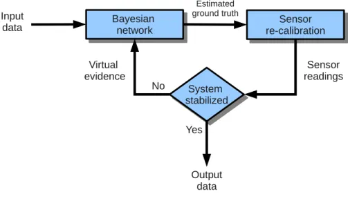
Figure 1 shows the overview of our system. It describes the high-level composition of the system. There are two major components, which are Bayesian network and sensor re-calibration. In the real-world applications, the gathered atmosphere data, e.g., O₃, is

10

processed by the system. The system can reduce the sensing error caused by drift as well as other atmospheric parameters, and re-calibrate the sensor function. The output of the system is the O₃data with significantly improved accuracy and a more sensitive sensor function.

The input of the system is the raw analog sensor readings in the form of voltage

15

or resistance. Note that actual ground truth readings are not required and only used for evaluation. The input sensor readings are first processed using a Bayesian belief network, which is trained with normal data from the in-field deployment. The Bayesian network can generate the estimated ground truth readings based on the readings from all the correlated sensors. The estimated ground truth readings are then used to

re-20

calibrate the sensors, i.e., generate the new sensor functions which can translate the input analog readings into pollutant concentration in the unit of parts per million (ppm). The new sensor functions are used to generate the sensor concentration readings, which can derive the error distribution together with the estimated ground truth. The error distribution can be used to update the virtual evidence of the Bayesian network.

25

(8)

AMTD

8, 8971–9008, 2015

Y. Xiang et al.

Title Page

Tables Figures

◭ ◮

Back Close

Full Screen / Esc

Discussion

P

a

per

|

Discussion

P

a

per

|

Discussion

P

a

per

|

Discussion

P

a

per

|

truth, thus forming a loop. If the system is stabilized, the loop exits and the recovered sensor readings are produced.

5 Basic Bayesian belief network

In this section, we first introduce the basic Bayesian belief network. Then we discuss how to implement it in real-world applications.

5

5.1 Bayesian network introduction

Bayesian networks are widely used to detect and recover abnormal data points for sensor networks. The Bayesian network is built based on Bayes’ theorem and capable of exploiting the inter-dependent or causal relationships of correlated sensors readings. The types of the sensors involved can be different, which makes it appropriate for our

10

application. A Bayesian network is a directed graph consisting of nodes and arcs (Kay, 1998).

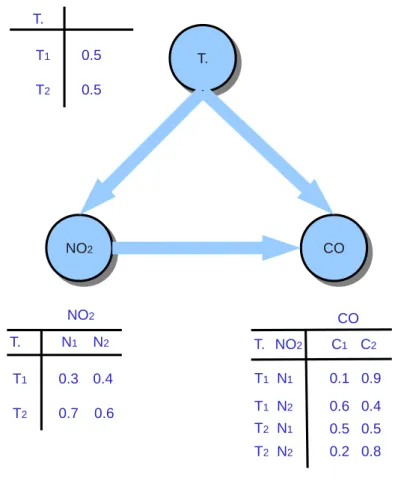
Figure 2 shows an example Bayesian belief network for a simple sensor network. In this application, there are three different types of sensors, which can measure tem-perature (T), carbon monoxide (CO), and nitrogen dioxide (NO2), respectively. Each

15

sensors’ readings can be discretized intonvalues, with each discrete value denoted as T_n, C_n, and N_n, respectively. Without loss of generality, we assume two distinct discrete values for each sensor type. All the sensors are correlated. The readings of metal oxide sensors are strongly affected by the temperature. Moreover, the readings of the NO₂sensor and CO sensor are also correlated with each other because of cross

20

sensitivity.

As shown in the figure, the Bayesian network describing this sensor network contains three nodes, with each representing one type of sensor. There are two arcs connecting the temperature sensor with the metal oxide sensors and one arc connecting the two metal oxide sensors. To calculate the probability inference of each variable given the

(9)

AMTD

8, 8971–9008, 2015

Y. Xiang et al.

Title Page

Tables Figures

◭ ◮

Back Close

Full Screen / Esc

Discussion

P

a

per

|

Discussion

P

a

per

|

Discussion

P

a

per

|

Discussion

P

a

per

|

input of other variables as evidence, each node is associated with a table, which is called conditional probability table (CPT). CPT describes the conditional dependence between any node with its parents. For the root node with no parents, CPT describes the distribution of the variable itself. CPT can be derived by training the network using historic data.

5

5.2 Bayesian network for real-world applications

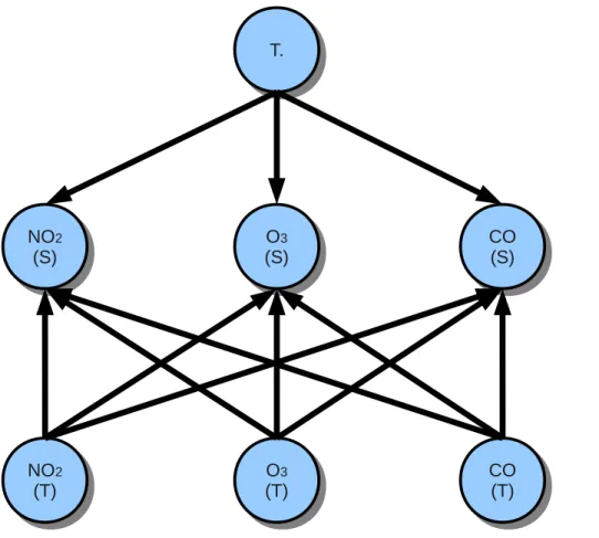
In this section, we discuss how to apply the Bayesian network technique to air quality monitoring application using mobile sensing devices equipped with multiple types of sensors. Without loss of generality, we assume that there are four types of equipped sensors: temperature, NO2, CO, and ozone (O3). Their readings are all correlated.

10

The Bayesian network graph for this application is shown in Fig. 3. In the graph, there are two types of nodes. The first type, which contains T, CO(S), NO2(S), and O3(S), represent the readings of the sensors. The second type, which contains CO(T), NO2(T), and O₃(T), represents the actual concentration (ground truth) of the corresponding pollutants in the environment. In the rest of paper, if a pollutant is followed by S, we

15

refer to the sensor reading of that pollutant. While if it is followed by T, we refer to its ground truth concentration.

In the figure, there are arrows connecting the temperature sensor to all the three types of metal oxide sensors since the readings of the temperature sensor influences them all. The metal oxide sensors are assumed to be independent from each other,

20

and the same is true for the ground truth concentration nodes. However, because of cross sensitivity, each ground truth reading can have significant impact on the readings of three metal oxide sensors simultaneously. Thus, there are three arcs connecting the ground truth concentrations to all the three sensors. When the ground truth is not available, the probability inference of the three ground truth nodes can be calculated

25

(10)

AMTD

8, 8971–9008, 2015

Y. Xiang et al.

Title Page

Tables Figures

◭ ◮

Back Close

Full Screen / Esc

Discussion

P

a

per

|

Discussion

P

a

per

|

Discussion

P

a

per

|

Discussion

P

a

per

|

6 Bayesian network with sensor re-calibration

In this section, we first talk about the problems of the basic Bayesian network for real-world applications in which sensors may drift. Then we introduce virtual evidences to address the drift problem and the sensor re-calibration technique to improve the per-formance of the Bayesian network. Finally, we present the combined recursive system

5

and describe the details and algorithm to implement it.

6.1 Problems for basic Bayesian network

Bayesian network can clean the corrupted data and detect abnormal readings by lever-aging the inter-dependency of correlated sensors. For the random noises, it is quite efficient and sufficient. However, in our applications, sensors frequently drift. It has

10

been shown, both by existing literature (Xiang et al., 2012; Romain and Nicolas, 2010) and by our own measurement data presented in Sect. 7.1.3, that sensor drift is a very common and severe problem in real-world applications for those metal oxide sensors. Significant drift can be accumulated within just a couple of months, making the sensors effectively useless afterwards if not re-calibrated. Thus, the problem of sensor drift and

15

the error caused by drift must be addressed.

The basic Bayesian belief network approach described in Sect. 5 cannot address the drift problem. Drift can be considered a systematic deviation of the sensor readings from the ground truth caused by the changing of the sensor function. When multiple sensors drift, the basic Bayesian network approach can no longer identify the abnormal

20

readings, let alone correct them and recover the ground truth. For example, consider a Bayesian network containing three nodes, which represent CO, NO2, and O3, respec-tively. Assume that the CO and NO₂sensors are drifted and constantly report extreme values that can rarely be observed in the normal environment. In that case, even if the ozone sensor is not drifted, the results of the Bayesian network can still be erroneous

25

(11)

AMTD

8, 8971–9008, 2015

Y. Xiang et al.

Title Page

Tables Figures

◭ ◮

Back Close

Full Screen / Esc

Discussion

P

a

per

|

Discussion

P

a

per

|

Discussion

P

a

per

|

Discussion

P

a

per

|

drifted sensors. Note that it is quite common to have more than one drifted sensors in the system simultaneously, as shown by our deployment results in Sect. 7.1. Thus, the system described in Fig. 3 is inadequate to address the real-world problems. To ap-ply the Bayesian network in such circumstances, we need to (1) incorporate a ranking mechanism that can quantify the sensor uncertainties into the Bayesian network and

5

(2) design a drift compensation scheme to re-calibrate the sensor function and recover the corrupted data simultaneously within the Bayesian network framework.

6.2 Error distribution and uncertain evidences

As the sensor drifts, its sensing sensitivity deteriorates and the uncertainty of its read-ings increases. A Bayesian network treats all its input equally, which is problematic

10

considering sensor drifts. For example, if a CO sensor is recently calibrated while an O3sensor has not been calibrated for a long time, we should clearly give the CO sen-sor more confidences. In other words, within a Bayesian network framework, we must have an evaluation mechanism which can rank and quantify the trustworthiness of each particular sensor.

15

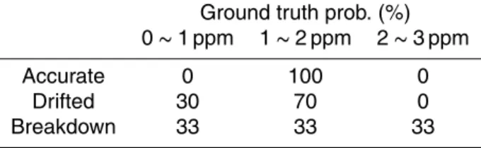
To address this problem, we use error distributions to represent the sensitivity and trustworthiness of the sensors. An example of error distributions is shown in Table 1. In the example, we assume that the sensor has reported an environment concentration of 1.5 ppm. The actual ground truth ranges from 0 to 3 ppm and is divided into three discrete categories. We assume that in the environment the probability for the ground

20

truth to be in any of these three categories is equal. As shown in Table 1, if the sensor is accurate, then the probability that the actual ground truth is within the range of 1 to 2 ppm given a reported reading of 1.5 ppm is 100 %. If the sensor is drifted, the sensor becomes less accurate and the possible value of the ground truth spreads wider. If the sensor has a breakdown, it loses most of its sensitivity and the ground truth is no

25

longer correlated to the sensor readings.

(12)

AMTD

8, 8971–9008, 2015

Y. Xiang et al.

Title Page

Tables Figures

◭ ◮

Back Close

Full Screen / Esc

Discussion

P

a

per

|

Discussion

P

a

per

|

Discussion

P

a

per

|

Discussion

P

a

per

|

the Bayesian network is called virtual evidence. Note that virtual evidence cannot be applied to the Bayesian network directly. The Bayesian network must be modified to incorporate such uncertain evidences.

6.3 Bayesian network with virtual evidence

For the basic Bayesian network, the inputs can only be determined values. To

incor-5

porate the virtual evidences, some constraints, which is called Je_ffrey’s rule (Je_ffrey, 1990), must be honored. The concept of Jeffrey’s rule is described as follows.

Suppose the universe of all the events is denoted asU. We have a set of mutually exclusive eventsγ₁,. . .,γ_n, which is a subset ofU, andP is the probability distribution of those events. After applying the virtual evidence, the beliefs for events γ1,. . .,γn

10

change and the updated distribution is denoted asP′.P′ should satisfy the following equation.

P(α|γ_i)=P′(α|γ_i), ∀i =1,. . .,n. (1) whereα is any event in the universe. In other words, after the virtual evidence is ac-cepted, the posterior probability ofαcan be changed, but the conditional probability for

15

α∈U regarding to the eventsγ1,. . .,γnmust remain the same.

To treat the virtual evidence as determined value while honoring the Jeffrey’s rule, the Bayesian network should be modified by adding a virtue node to the drifted sensor nodes (Chan and Darwiche, 2005). Figure 4 shows an example Bayesian network with virtual nodes. In the figure, the pollutant followed byV represent a virtual node in the

20

Bayesian network. The number in the table is the conditional probability.λrepresents the probability distribution of the input evidence. There are two sensor nodes, which are temperature and CO. The temperature sensor is assumed to be accurate and with little drift, while the CO sensor can drift. The CO sensor node is associated with a virtual node, denoted as CO(V). The virtual node also has its own conditional probability table.

25

(13)

AMTD

8, 8971–9008, 2015

Y. Xiang et al.

Title Page

Tables Figures

◭ ◮

Back Close

Full Screen / Esc

Discussion

P

a

per

|

Discussion

P

a

per

|

Discussion

P

a

per

|

Discussion

P

a

per

|

Jeffrey’s rule. The detailed methods and equations to calculate its probability table can be found in existing literature (Peng et al., 2010; Chan and Darwiche, 2005). Note that the virtual node is only dependent on the corresponding sensor node and independent of all the other nodes in the network.

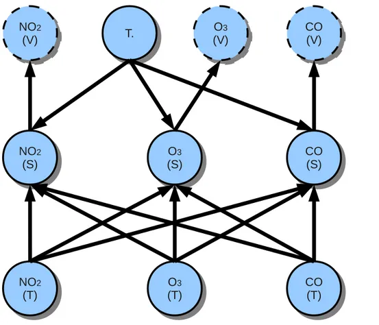
Figure 5 shows the Bayesian network structure of our application after incorporating

5

the virtual evidences. The definition of the symbols can be found in Sect. 5.2. Since the temperature sensor and the hypothetical ground truth concentration sensors are assumed to be accurate, they are not associated with any virtual nodes. Each metal oxide sensor, which is prone to drift, is associated with a virtual node. The contents in the CPT of the virtual nodes can be calculated using the error distributions of the

10

actual nodes, which can be derived with the information of the (estimated) ground truth readings and the sensor readings.

6.4 Sensor function re-calibration

The transformation function to translate the analog input signal into pollutant concen-tration is called a sensor calibration function, or sensor function. The abnormal

read-15

ings caused by environmental noises do not reflect a change of the sensor function. However, when sensors are drifted, the sensor functions change, which can cause a systematic increase of abnormal readings.

In this work, we apply a piece-wise linear function as the sensor function, which is shown in the following equation.

20

C=p1+p2·V +p3·T, (2)

whereC is the pollutant concentration,pi are the fitting parameters, V is the voltage, and T is the temperature. The temperature information is reported by the on-board sensors. The parameters in the equation are derived using linear regression with the training data. Since accurate sensors providing ground truth readings are usually not

25

(14)

AMTD

8, 8971–9008, 2015

Y. Xiang et al.

Title Page

Tables Figures

◭ ◮

Back Close

Full Screen / Esc

Discussion

P

a

per

|

Discussion

P

a

per

|

Discussion

P

a

per

|

Discussion

P

a

per

|

of this re-calibration scheme deteriorates. When a sensor breaks down and loses most of its sensitivity, the sensor can no longer be re-calibrated.

6.5 System design

Figure 6 shows the flow of our system. The input sensor readings are first processed using a Bayesian belief network, which is trained using normal data from the in-field

5

deployment. The Bayesian network can generate the estimated ground truth values based on the conditional probability tables and readings from all the correlated sen-sors. The estimated ground truth readings are then used to re-calibrate the sensors, i.e., generate the new sensor functions which can translate the input sensor analog readings into actual pollutant concentrations. The new sensor functions are used to

10

generate the sensor readings, which are used to derive the estimated error. The newly updated estimated error is compared with the previous estimations. If the variation is within a certain threshold, we consider the system stabilized and the current results are the best estimation and final output. If the system is not stabilized yet, the virtual evidence, which describes the error distributions of the input data, is updated using the

15

(15)

AMTD

8, 8971–9008, 2015

Y. Xiang et al.

Title Page

Tables Figures

◭ ◮

Back Close

Full Screen / Esc

Discussion

P

a

per

|

Discussion

P

a

per

|

Discussion

P

a

per

|

Discussion

P

a

per

|

Algorithm 1Algorithm for the Implementation of the System Require: S // The input analog readings

Require: B// The trained Bayesian network Require: O// The output set

Require: V // The initial distributions of the virtual evidences Require: F // The initial sensor calibration function

N←si ze(S) O←F(S)

E ←∅,E is the estimated ground truth set whileOdoes not convergedo

fori=1 :N do E(i)←B(V(i),S(i)) end for

F ←Li near_regressi on(E,S) O←F(S)

UpdateV usingOandE end while

7 Experimental results

In this section, we first describe a real-world co-location deployment of 9 mobile sensor nodes and the analysis results for the deployment data. We then evaluate our system using the real-world data.

7.1 Mobile sensor network deployment and analysis

5

(16)

AMTD

8, 8971–9008, 2015

Y. Xiang et al.

Title Page

Tables Figures

◭ ◮

Back Close

Full Screen / Esc

Discussion

P

a

per

|

Discussion

P

a

per

|

Discussion

P

a

per

|

Discussion

P

a

per

|

7.1.1 The mobile sensing device

To investigate the effect of sensor drift in real-world applications and collect data to eval-uate our data cleaning technique, we deployed a sensor network in Denver, Colorado. During the experiment, we deployed 9 M-Pods (Jiang et al., 2011), which are shown in Fig. 7. The M-Pod is a custom-built mobile sensing device supporting embedded

5

sensing, computation, and wireless communication. It supports detection of various air pollutants, including NO₂, CO, CO₂, O₃, and VOCs. It can also measure temperature, humidity, and light. The latest revision of the M-Pod is compact (5 cm×6.5 cm) and energy efficient, with a battery life of greater than 16 h. The whole device, including a Li-ion battery with a capacity of 6000 mAh, is enclosed by a low-cost off-the-shelf

10

case that can be carried using an armband or attached to a backpack. A 3.3 V DC fan is used to control airflow. A rectangular filter is installed around sensor to increase sensing accuracy and prolong sensor life. Most of the power hungry on-board sensors are power gated and can be controlled by commands from smartphones. Data are tem-porally stored in a one megabyte non-volatile EEPROM. The total cost of the on-board

15

components and sensors is less than USD 150 and can be reduced further if produced in large quantity.

To receive, store, and present the data gathered by our M-Pod device, we have devel-oped on-board firmware, smartphone applications, data servers, and web interfaces. The firmware defines protocols of sensing, storing, and sending the environmental

20

data. The smartphone application communicates with the M-Pod via its Bluetooth in-terface. It can issue commands to and receive data from the M-pod. The data are transmitted to the on-line data server and stored in the databases. A web-based user interface allows users to access and analyze air quality data.

7.1.2 The real world deployment

25

(17)

AMTD

8, 8971–9008, 2015

Y. Xiang et al.

Title Page

Tables Figures

◭ ◮

Back Close

Full Screen / Esc

Discussion

P

a

per

|

Discussion

P

a

per

|

Discussion

P

a

per

|

Discussion

P

a

per

|

by users as part of an exposure assessment study. During three multi-day calibration periods in March, April, and May, the M-Pods were placed at a reference air quality monitoring site. The M-Pods were powered continuously on the roof of the monitoring building, in a ventilated enclosure near the air inlets for the reference monitors. The reference site, as shown in Fig. 7, monitors CO, NO2, and O3. It is located in

down-5

town Denver, Colorado, and operated by the Colorado Department of Public Health and Environment (CDPHE). The highly accurate and regularly maintained air pollutant monitoring equipment in the station is used to provide the ground truth readings.

By co-locating the M-Pods with the reference monitors, we are able to derive both the sensor analog readings and ground truth, which can be used to determine the sensor

10

calibration functions. The forms of the sensor calibration functions vary depending on sensor type. In this work, we use a piece-wise linear function. It is quite accurate ac-cording to lab and field measurements, and requires much less resources to compute compared with other more complicated forms of sensor functions. The calibrations are performed using the field data. Thus, it does not require specialized equipment, and

15

can cover a wider range of environmental parameter space than lab calibrations. Be-fore the fitting of the sensor function, data filtering was performed to remove noise from the sensor readings. Minute medians were first calculated from the 6 s raw data. Then, we applied a filter based on difference in consecutive differences in the medians. There were two thresholds for the filter, an absolute threshold that was deemed

unre-20

alistic based on lab experiments, and 2 times the standard deviation of the differences. By performing calibrations periodically with the same sets of sensors, we were able to assess the change in baseline readings and sensitivity over time. The calibration func-tions derived by fitting to the data of the first calibration period, which is considered as the undrifted baseline, are applied to the entire data set.

25

7.1.3 Data analysis

(18)

AMTD

8, 8971–9008, 2015

Y. Xiang et al.

Title Page

Tables Figures

◭ ◮

Back Close

Full Screen / Esc

Discussion

P

a

per

|

Discussion

P

a

per

|

Discussion

P

a

per

|

Discussion

P

a

per

|

An example of the measured data and the corresponding ground truth readings is presented in Fig. 8. The X axis in the figure shows the time line of the deployment in the unit of days, while theY axis shows the concentration of the pollutant in parts per million. Two sets of data are presented. The red dots represent the ground truth data measured by the accurate and regularly maintained equipment in the monitoring

5

station, while the blue dots represent the data measured by the less accurate and drift-prone metal oxide sensors housed by the M-Pods. The total duration of the deployment is about two months. In the figure, there are three separate time periods, with each lasting for about one week. During that time period, the M-Pods are located in the station and calibrating. For the rest of the time, the M-Pods are carried by individual

10

users and the ground truth readings of their exposed environments are unknown. Thus, the readings from those time periods are not included.

The resultant data show that the drift rates for different types of sensors vary. For the example in the figure, the NO₂ sensor experiences large drift. After two months, its error is increased more than 3 times. The CO sensor also suffers significant drift,

15

though less compared to the NO2 sensor with about 50 % increase of error. But for the O₃sensor, no significant drift is observed. The example shows that significant drift can occur within just a couple of months, rendering the corresponding sensor almost useless if not carefully re-calibrated. It demonstrated that drift is a real and severe challenge for those cheap sensors to be useful in real-world applications. Moreover,

20

since the exposed environment and the properties of the sensors vary, different sensors usually exhibit different drift rates, making it impossible to re-calibrate the sensors using a predetermined model.

Among the 9 M-Pods deployed, we choose 6 of them during our analysis and evalu-ations. For the rest three, one of them did not return enough data due to transmission

25

(19)

AMTD

8, 8971–9008, 2015

Y. Xiang et al.

Title Page

Tables Figures

◭ ◮

Back Close

Full Screen / Esc

Discussion

P

a

per

|

Discussion

P

a

per

|

Discussion

P

a

per

|

Discussion

P

a

per

|

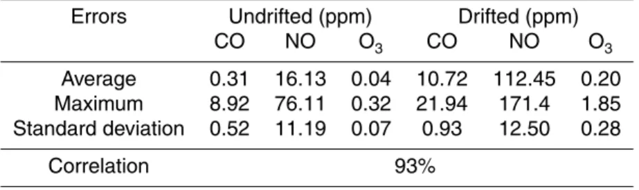
data are taken from the first time period as shown in Fig. 8. The drifted data are taken from the third time period. The first three columns shows the average, maximum, and standard deviation of the error distributions. Significant drift can be observed for all the types of sensors. It should be noted that for some pollutants, such as NO₂ and CO, their mean values change more significantly than the standard deviation, which implies

5

a close to linear shift. The last column of the table shows the correlation percentage. Correlation percentage is defined as the percentage of the sensor pairs that shows strong correlation among all the possible pairs of all the sensors. The result shows a correlation percentage of over 93 %, indicating that Bayesian network might be an appropriate solution.

10

In conclusion, our deployment data show that sensor drift and consequently the noise problem are very realistic and important for the metal oxide sensors. If not properly ad-dressed, most of those sensors can be useless within just a couple of months. The drift rates are dependent on the environment and sensor properties and hence, vary for different sensors. Thus, it is not feasible to use predetermined correction methods:

15

sensor calibration problem must be addressed using the field data. Moreover, diff er-ent types of sensors show strong correlations, permitting noise reduction and sensor calibration.

7.2 Data recovery and sensor calibration results

In this section, we discuss the experimental environment setup and contrast our

tech-20

nique with the alternatives.

7.2.1 Experiment setup

The outlier cleaning and sensor re-calibration functions are written using Matlab, with the help of an external Bayesian network toolbox called bnt (Bayes Toolbox, 2007). The program runs on a 4-core Intel Xeon E31230 machine with 8 GB memory. We

25

(20)

AMTD

8, 8971–9008, 2015

Y. Xiang et al.

Title Page

Tables Figures

◭ ◮

Back Close

Full Screen / Esc

Discussion

P

a

per

|

Discussion

P

a

per

|

Discussion

P

a

per

|

Discussion

P

a

per

|

the failed sensors and sensors with insufficient data. The failed sensors are not used since their readings are no longer correlated with each other and re-calibration cannot help improve the results. In other words, our technique does not have effect on them and they should be simply replaced. The failed sensor can be detected using both our technique and the Bayesian network method. The threshold to determine the outliers

5

is equal to the standard deviation of the ground truth readings.

The CPT of the Bayesian network is derived from training. The training set is gen-erated using the co-location data from undrifted (the first) time period. This approach is more appropriate since it require much less effort to cover a reasonable number of states than lab environment, and can provide us a more realistic prior distributions for

10

temperature. The training dataset is filtered so that it contains only normal data. After the Bayesian network is trained, the contents in the CPT remain unchanged until the sensor is close to a reference station and have access to the ground truth readings again. For the parameter states that are not encountered during the training phase, we replace their contents with the encountered state of the closest distance, calculated

15

using the Euclidean distance between those two states.

To evaluate our outlier recovery and sensor re-calibration technique, we compare the following three approaches.

1. Uncompensated. This approach interprets the reported analog data using the pre-determined sensor function from lab measurement and without any compensation

20

scheme.

2. Bayesian network. This approach implements a Bayesian belief network based technique proposed by Janakiram et al. (2006). It is the most relevant and closely related work to the best of our knowledge.

3. Our technique. It improved upon the Bayesian network approach by incorporating

25

the virtual evidence and sensor re-calibration.

(21)

AMTD

8, 8971–9008, 2015

Y. Xiang et al.

Title Page

Tables Figures

◭ ◮

Back Close

Full Screen / Esc

Discussion

P

a

per

|

Discussion

P

a

per

|

Discussion

P

a

per

|

Discussion

P

a

per

|

7.2.2 Drifted sensor recovery evaluation

Many existing outlier detection approaches, such as distance based techniques (Pa-padimitriou et al., 2003; Subramaniam et al., 2006) or classification based techniques (Rajasegarar et al., 2007), cannot estimate the ground truth data and provide re-calibration opportunities for the drifted sensors. Thus, we do not include them in the

5

comparison. Figure 9 shows the performance of various relevant data cleaning and recovery techniques. Since our technique focuses on the sensor drift and re-calibration problem, the experiment is performed on the third time period of the data set, which represents the drifted sensors. TheY axis of the bar graph shows the average errors, which are normalized to our recursive technique. The red numbers above the bar show

10

the actual average error value for the uncompensated method. Compared with the un-compensated approach, in which the sensor outliers are not un-compensated and sensor calibration functions are not re-calibrated, our technique can incur only about 2.13 % error on average. Moreover, compared with the Bayesian network approach, which is the closest existing technique, our technique is capable of reducing errors by 32.0,

15

34.7, and 35.5 % for CO, NO₂, and O₃, respectively. Overall, our technique can reduce error by 34.1 % on average.

After the estimated ground truth values are derived, we consider it as the ground truth concentration. However, since the ground truth concentration estimation is im-perfect, the classification of sensor readings according to this estimate ground truth

20

concentrations can be wrong. Hereby we define data recovery rate as the percentage of corrected label data points after the data recovery scheme. Figure 10 shows the comparison results of various techniques in terms of data recovery rate. The rate is obtained by comparing the estimated readings against the ground truth. For our tech-nique, the data recovery rates are 34.7, 33.3, 41.3 % for CO, NO₂, and O₃, respectively.

25

(22)

AMTD

8, 8971–9008, 2015

Y. Xiang et al.

Title Page

Tables Figures

◭ ◮

Back Close

Full Screen / Esc

Discussion

P

a

per

|

Discussion

P

a

per

|

Discussion

P

a

per

|

Discussion

P

a

per

|

7.3 Outlier detection and cross sensitivity

In addition to the data recovery and sensor function re-calibration for the drifted data, our technique is also capable of detecting outlier readings caused by random noise dur-ing undrifted period. The testdur-ing dataset in this case consists of undrifted data points, which are from the first time period. Since during normal operation, the outliers are

5

quite scarce, we create the testing dataset by manually setting the ratio of normal and abnormal data points. We first pick all the abnormal readings from the dataset, then randomly choose the same number of random samples. Thus, in the testing set, the ratio of abnormal readings is set to be 50 %. The detection rate is the combined correct classification ratio by excluding the false positives and false negatives. We compare

10

the outlier detection efficiency of our technique and the Bayesian network approach. The results are shown in Fig. 11. The performance of our technique and the Bayesian network is quite similar, both having a detection rate of about 87 %. This is as expected since during normal operation, the sensors are not drifted and thus, sensor function re-calibration should not have any significant impact on the results.

15

In addition to the outlier detection and drift compensation, another advantage of our technique, as well as the Bayesian network approach, is that it can automatically iden-tify the pollutant composition in the air, thus addressing the cross sensitivity problem. In the real-world deployment, the deployment environment is often complex and het-erogeneous. Therefore, without the knowledge of the pollutant composition in the air,

20

it is very hard to get an accurate estimation of the pollutant concentration using the metal oxide sensors. Our technique can identify and quantify the pollutants in the air as long as they are previously included in the training set. However, the total number of pollutants in our system should be limited due to the constraint of storage space requirement.

(23)

AMTD

8, 8971–9008, 2015

Y. Xiang et al.

Title Page

Tables Figures

◭ ◮

Back Close

Full Screen / Esc

Discussion

P

a

per

|

Discussion

P

a

per

|

Discussion

P

a

per

|

Discussion

P

a

per

|

8 Conclusions

In this work, we have presented a Bayesian belief network based system to detect and recover outliers in the presence of sensor drift. This work is to address the data noise and sensor drift problems in the atmosphere research by exploring the correlation of different types of sensors. In our analysis of real-world data, sensors usually incur

5

significant drift within a few months. Thus, to ensure the accuracy of the atmosphere researches utilizing those sensors, we develop a data treatment technique that can significantly reduce the sensor noise and re-calibrate the drifted sensor online.

Our method improves upon the state-of-art Bayesian belief network techniques by incorporating the virtual evidence and adjusting the sensor calibration functions

re-10

cursively. We have also performed a real-world deployment of mobile sensor network to investigate sensor drifts and validate our technique. Compared with the existing Bayesian network technique, our method can improve the result significantly. As a re-sult, our technique can reduce error by 34.1 % and increase the recovered data rate by 4 times on average.

15

References

Arshak, K., Moore, E., Lyons, G. M., Harris, J., and Clifford, S.: A review of gas sensors em-ployed in electronic nose applications, Sensor Rev., 24, 181–198, 2004. 8973

Bayes Toolbox: Bayes Net Toolbox for Matlab, available at: https://code.google.com/p/bnt/ (last access: 26 August 2015), 2007. 8989

20

Bettencourt, L. M., Hagberg, A., and Larkey, L.: Separating the wheat from the chaff: practical anomaly detection schemes in ecological applications of distributed sensor networks, in: Distributed Computing in Sensor Systems, Springer Berlin Heidelberg, Germany, vol. 4549, 223–239, 2007. 8976

Bychkovskiy, V., Megerian, S., Estrin, D., and Potkonjak, M.: A collaborative approach to in-25

(24)

AMTD

8, 8971–9008, 2015

Y. Xiang et al.

Title Page

Tables Figures

◭ ◮

Back Close

Full Screen / Esc

Discussion

P

a

per

|

Discussion

P

a

per

|

Discussion

P

a

per

|

Discussion

P

a

per

|

Chan, H. and Darwiche, A.: On the revision of probabilistic beliefs using uncertain evidence, Artif. Intell., 163, 67–90, 2005. 8982, 8983

Chandola, V., Banerjee, A., and Kumar, V.: Anomaly detection: a survey, ACM Comput. Surv., 41, 15 pp., 2009. 8973

Di Lecce, V. and Calabrese, M.: Discriminating gaseous emission patterns in low-cost sensor 5

setups, in: Proc. Int. Conf. Computational Intelligence for Measurement Systems and Appli-cations, Ottawa, ON, Canada, 19–21 September 2011, 1–6, 2011. 8973

Elnahrawy, E. and Nath, B.: Cleaning and querying noisy sensors, in: Proc. Int. Conf. Wireless Sensor Networks and Applications, San Diego, CA, USA, 19 September 2003, 78–87, 2003. 8973, 8976

10

Haugen, J.-E., Tomic, O., and Kvaal, K.: A calibration method for handling the temporal drift of solid state gas-sensors, Anal. Chim. Acta, 407, 23–39, 2000. 8973

Janakiram, D., Adi Mallikarjuna Reddy, V., and Phani Kumar, A.: Outlier detection in wireless sensor networks using Bayesian belief networks, in: Proc. Int. Conf. Communication System Software and Middleware, Delhi, India, 8–12 January 2006, 1–6, 2006. 8974, 8977, 8990 15

Jeffrey, R. C.: The Logic of Decision, University of Chicago Press, Chicago, USA, 1990. 8982 Jiang, Y., Li, K., Tian, L., Piedrahita, R., Xiang, Y., Mansata, O., Lv, Q., Dick, R. P.,

Hanni-gan, M., and Shang, L.: MAQS: a personalized mobile sensing system for indoor air qual-ity monitoring, in: Proc. Int. Conf. Ubiquitous Computing, Beijing, China, 17–21 September 2011, 271–280, 2011. 8972, 8974, 8986

20

Kay, S. M.: Fundamentals of Statistical Signal Processing, Volume 2: Detection Theory, Prentice Hall PTR, Upper Saddle River, NJ, USA, 1998. 8978

Kumar, D., Rajasegarar, S., and Palaniswami, M.: Automatic sensor drift detection and correc-tion using spatial kriging and kalman filtering, in: Proc. Int. Conf. Distributed Computing in Sensor Systems, Cambridge, MA, USA, 20–23 May 2013, 183–190, 2013. 8976

25

Miluzzo, E., Lane, N., Campbell, A., and Olfati-Saber, R.: CaliBree: a self-calibration system for mobile sensor networks, in: Proc. Int. Conf. Distributed Computing in Sensor Systems, vol. 5067, Santorini, Greece, 11–14 June 2008, 314–331, 2008. 8975

Papadimitriou, S., Kitagawa, H., Gibbons, P., and Faloutsos, C.: LOCI: fast outlier detection using the local correlation integral, in: Proc. Int. Conf. Data Engineering, Bangalore, India, 30

5–8 March 2003, 315–326, 2003. 8976, 8991

(25)

AMTD

8, 8971–9008, 2015

Y. Xiang et al.

Title Page

Tables Figures

◭ ◮

Back Close

Full Screen / Esc

Discussion

P

a

per

|

Discussion

P

a

per

|

Discussion

P

a

per

|

Discussion

P

a

per

|

Piedrahita, R., Xiang, Y., Masson, N., Ortega, J., Collier, A., Jiang, Y., Li, K., Dick, R. P., Lv, Q., Hannigan, M., and Shang, L.: The next generation of low-cost personal air quality sensors for quantitative exposure monitoring, Atmos. Meas. Tech., 7, 3325–3336, doi:10.5194/amt-7-3325-2014, 2014. 8972

Rajasegarar, S., Leckie, C., Palaniswami, M., and Bezdek, J.: Quarter sphere based distributed 5

anomaly detection in wireless sensor networks, in: Proc. Int. Conf. Communications, Glas-gow, UK, 24–28 June 2007, 3864–3869, 2007. 8976, 8991

Romain, A. and Nicolas, J.: Long term stability of metal oxide-based gas sensors for e-nose en-vironmental applications: an overview, Sensor. Actuat. B-Chem., 146, 502–506, 2010. 8973, 8980

10

Subramaniam, S., Palpanas, T., Papadopoulos, D., Kalogeraki, V., and Gunopulos, D.: Online outlier detection in sensor data using non-parametric models, in: Proc. Int. Conf. Very Large Data Bases, Seoul, South Korea, 12–15 September 2006, 187–198, 2006. 8991

Tans, P. and Thoning, K.: How we measured background CO₂levels on Mauna Loa, available at: http://www.esrl.noaa.gov/gmd/ccgg/about/co2_measurements.html, last access: Septem-15

ber, 2008. 8973

Willett, W., Aoki, P., Kumar, N., Subramanian, S., and Woodruff, A.: Common sense community: scaffolding mobile sensing and analysis for novice users, in: Pervasive Computing, Helsinki, Finland, 17–20 May 2010, 6030, 301–318, 2010. 8972, 8974

Xiang, Y., Bai, L. S., Piedrahita, R., Dick, R. P., Lv, Q., Hannigan, M. P., and Shang, L.: Col-20

laborative calibration and sensor placement for mobile sensor networks, in: Proc. Int. Symp. Information Processing in Sensor Networks, Beijing, China, 16–19 April 2012, 73–84, 2012. 8975, 8980

Xiang, Y., Piedrahita, R., Dick, R., Hannigan, M., Lv, Q., and Shang, L.: A hybrid sensor system for indoor air quality monitoring, in: Proc. Int. Conf. Distributed Computing in Sensor Systems, 25

Cambridge, MA, USA, 20–23 May 2013, 96–104, 2013. 8975

Zampolli, S., Elmi, I., Ahmed, F., Passini, M., Cardinali, G., Nicoletti, S., and Dori, L.: An elec-tronic nose based on solid state sensor arrays for low-cost indoor air quality monitoring ap-plications, Sensor. Actuat. B-Chem., 101, 39–46, 2004. 8973

Zhang, Y., Meratnia, N., and Havinga, P.: Outlier detection techniques for wireless sensor net-30

(26)

AMTD

8, 8971–9008, 2015

Y. Xiang et al.

Title Page

Tables Figures

◭ ◮

Back Close

Full Screen / Esc

Discussion

P

a

per

|

Discussion

P

a

per

|

Discussion

P

a

per

|

Discussion

P

a

per

|

Table 1.An Example Error Distribution with Reported Reading of 1.5 ppm.

Ground truth prob. (%) 0∼1 ppm 1∼2 ppm 2∼3 ppm

Accurate 0 100 0

Drifted 30 70 0

(27)

AMTD

8, 8971–9008, 2015

Y. Xiang et al.

Title Page

Tables Figures

◭ ◮

Back Close

Full Screen / Esc

Discussion

P

a

per

|

Discussion

P

a

per

|

Discussion

P

a

per

|

Discussion

P

a

per

|

Table 2.The Statistics of the Original and Drifted Sensor Readings.

Errors Undrifted (ppm) Drifted (ppm)

CO NO O₃ CO NO O₃

Average 0.31 16.13 0.04 10.72 112.45 0.20

Maximum 8.92 76.11 0.32 21.94 171.4 1.85

Standard deviation 0.52 11.19 0.07 0.93 12.50 0.28

(28)

AMTD

8, 8971–9008, 2015

Y. Xiang et al.

Title Page

Tables Figures

◭ ◮

Back Close

Full Screen / Esc

Discussion

P

a

per

|

Discussion

P

a

per

|

Discussion

P

a

per

|

Discussion

P

a

per

|

Bayesian network Bayesian

network _{re-calibration}Sensor Sensor re-calibration Input

data

Estimated ground truth

Virtual evidence

System stabilized System stabilized

Output data

Sensor readings

Yes No

(29)

AMTD

8, 8971–9008, 2015

Y. Xiang et al.

Title Page

Tables Figures

◭ ◮

Back Close

Full Screen / Esc

Discussion

P

a

per

|

Discussion

P

a

per

|

Discussion

P

a

per

|

Discussion

P

a

per

|

T.

NO2

NO2 CO_CO

T1

T2

0.5

T.

T1

T2

0.3

0.7 NO2

T.

N1

N2

0.1

0.6 CO

NO2

N1 N2

0.4

0.6

T1

T.

N1

N2

T2

0.5

0.2 C1 C2

0.9

0.4

0.5

0.8

(30)

AMTD

8, 8971–9008, 2015

Y. Xiang et al.

Title Page

Tables Figures

◭ ◮

Back Close

Full Screen / Esc

Discussion

P

a

per

|

Discussion

P

a

per

|

Discussion

P

a

per

|

Discussion

P

a

per

|

T. T.

NO2 (S)

NO2

(S) CO_(S)

CO (S)

O3 (S)

NO2 (T)

NO2

(T) _(T)O3

O3

(T) CO_(T)

CO (T)

(31)

AMTD

8, 8971–9008, 2015

Y. Xiang et al.

Title Page

Tables Figures

◭ ◮

Back Close

Full Screen / Esc

Discussion

P

a

per

|

Discussion

P

a

per

|

Discussion

P

a

per

|

Discussion

P

a

per

|

T. T.

CO (V) CO

(V) COCO

T1

T2

0.5

CO

C1

C2

0.3

0.7

T.

0.1

0.6 CO

T1 T.

T2

C1 C2

0.9

0.4 λ

(32)

AMTD

8, 8971–9008, 2015

Y. Xiang et al.

Title Page

Tables Figures

◭ ◮

Back Close

Full Screen / Esc

Discussion

P

a

per

|

Discussion

P

a

per

|

Discussion

P

a

per

|

Discussion

P

a

per

|

T. T.

NO2

(S)

NO2

(S) CO_(S)

CO (S)

O3 (S)

NO2 (T)

NO2

(T) _(T)O3

O3

(T) CO_(T)

CO (T)

NO2

O3

CO

CO ( )

(33)

AMTD

8, 8971–9008, 2015

Y. Xiang et al.

Title Page

Tables Figures

◭ ◮

Back Close

Full Screen / Esc

Discussion

P

a

per

|

Discussion

P

a

per

|

Discussion

P

a

per

|

Discussion

P

a

per

|

Trained Bayesian network

Estimated truth value

Sensor readings

Sensor function re-calibration

Re-calibrated reading

Re-calibrated

reading _updateError

Error update

Virtual evidence

Error stabilized

Error

stabilized Corrected_reading

Corrected reading Yes

No

(34)

AMTD

8, 8971–9008, 2015

Y. Xiang et al.

Title Page

Tables Figures

◭ ◮

Back Close

Full Screen / Esc

Discussion

P

a

per

|

Discussion

P

a

per

|

Discussion

P

a

per

|

Discussion

P

a

per

|

(a) (b)