The sound speed anomaly of Baltic Seawater

(1)

OSD

12, 2565–2589, 2015

The sound speed anomaly of Baltic

Seawater

C. von Rohden et al.

Title Page

Abstract Introduction

Conclusions References

Tables Figures

◭ ◮

Back Close

Full Screen / Esc

Printer-friendly Version Interactive Discussion

Discussion

P

a

per

|

Discussion

P

a

per

|

Discussion

P

a

per

|

Discussion

P

a

per

|

Ocean Sci. Discuss., 12, 2565–2589, 2015 www.ocean-sci-discuss.net/12/2565/2015/ doi:10.5194/osd-12-2565-2015

This discussion paper is/has been under review for the journal Ocean Science (OS). Please refer to the corresponding final paper in OS if available.

The sound speed anomaly of Baltic

Seawater

C. von Rohden1, S. Weinreben2, and F. Fehres1

1

Physikalisch-Technische Bundesanstalt (PTB), Abbestr. 2–12, 10587 Berlin, Germany 2

Leibniz Institute for Baltic Sea Research, Seestr. 15, 18119 Warnemünde, Germany

Received: 4 September 2015 – Accepted: 2 October 2015 – Published: 2 November 2015

Correspondence to: F. Fehres (felix.fehres@ptb.de)

(2)

OSD

12, 2565–2589, 2015

Seawater

Title Page

Tables Figures

◭ ◮

Back Close

Full Screen / Esc

Discussion

P

a

per

|

Discussion

P

a

per

|

Discussion

P

a

per

|

Discussion

P

a

per

|

Abstract

The effect of the anomalous chemical composition of Baltic seawater on the speed of

sound relative to seawater with quasi-standard composition was quantified at

atmo-spheric pressure and temperatures of 1 to 46◦_{C. Three modern oceanographic}

time-of-flight sensors were applied in a laboratory setup for measuring the speed-of-sound

5

differenceδwin a pure water diluted sample of North Atlantic seawater and a sample of Baltic seawater of the same conductivity, i.e. the same Practical Salinity (SP=7.766).

The averageδw amounts to 0.069±0.014 m s−1, significantly larger than the

resolu-tion and reproducibility of the sensors and independent of temperature. This magnitude for the anomaly effect was verified with offshore measurements conducted at different

10

sites in the Baltic Sea using one of the sensors. The results from both measurements show values up to one order of magnitude smaller than existing predictions based on chemical models.

1 Introduction

An important issue regarding the quantification of thermodynamic properties of

seawa-15

ter with high accuracy is the natural variability of the relative composition of dissolved solutes. A certain variability of the thermodynamic properties should be connected with this. Although known for more than a century, these property anomalies came more into focus with the recent formulation of the equation of state of seawater (TEOS-10: IOC et al., 2010). TEOS-10 consistently represents all thermodynamic properties

20

of seawater at the high accuracy level required for modern oceanographic research and state-of-the-art modelling. It also supports the investigation of effects associated with composition anomalies. However, for a number of properties including the speed

of sound, there is a lack of experimental data with sufficient accuracy for a reliable

quantification of the anomaly effects.

(3)

OSD

12, 2565–2589, 2015

Seawater

Title Page

Tables Figures

◭ ◮

Back Close

Full Screen / Esc

Discussion

P

a

per

|

Discussion

P

a

per

|

Discussion

P

a

per

|

Discussion

P

a

per

|

TEOS-10 refers to Absolute Salinity SA as a basic input variable which quantifies

the total mass of all dissolved species in a unit mass of seawater. However,SA is not

directly measurable in practice. Salinity as a basic oceanographic measurand besides temperature and pressure is commonly determined from CTD measurements (con-ductivity, temperature, and pressure) according to the Practical Salinity Scale

(PSS-5

78, Perkin and Lewis, 1980). That means that the Practical SalinitySP as a measure

for salinity exclusively refers to electrically conductive solutes. Hence, for the

conver-sion of SP to SA at a high accuracy level, the natural variation of the relative

com-position of solutes as well as the contribution of non-ionic species have to be con-sidered. For the global ocean, this is implemented in TEOS-10 with an anomaly

cor-10

rection based on a mapped data set (McDougall et al., 2012). The salinity anomaly is described asδSA=SA−SR, referring to the conductivity based Reference Salinity

SR=SP×(35.16504/35) g kg− 1

as the best estimate of the Absolute Salinity of seawa-ter with a standard composition. Typically,δSA in the open ocean is small but

signifi-cant, reachingδSA=0.027 g kg− 1

in the northern North Pacific (IOC et al., 2010). This

15

equals a relative deviation of 0.077 % at Standard Seawater salinity. The main sources are additions of nutrients and carbonates (Millero et al., 2008). However, the effect may be larger in coastal and estuarine waters, mainly because of the increased influence of freshwater input from rivers, causing a significant effect on the related thermodynamic properties. Feistel et al. (2010a) state that currently the accuracy of the empirical

for-20

mulas for thermodynamic properties of seawater is easily limited by such e_ffects.

The Baltic Sea has brackish water, which is influenced by the Ca2+ and carbonate

dominated freshwater input from various rivers, and is therefore an especially good ex-ample. Extensive field measurements and studies on salinity and density shifts due to composition variability in the Baltic Sea have been conducted (e.g. Millero and

Krem-25

(4)

OSD

12, 2565–2589, 2015

Seawater

Title Page

Tables Figures

◭ ◮

Back Close

Full Screen / Esc

Discussion

P

a

per

|

Discussion

P

a

per

|

Discussion

P

a

per

|

Discussion

P

a

per

|

solutes. Sound speed is one of the quantities of fundamental interest due to its ther-modynamic relation to other properties, e.g. compressibility and density, and because of its large field of technical applications, e.g. in marine acoustics.

In this study we focus on the speed of sound and show measurement results

quan-tifying the sound speed difference which is associated with the anomalous chemical

5

composition of Baltic seawater. We applied modern acoustic time-of-flight sensors from

two different manufacturers under controlled laboratory conditions. The sensors,

de-signed for oceanographic in situ applications, provide sufficient resolution to resolve the speed-of-sound anomaly, independently of their reliability for absolute measure-ments and of the exact manner of sensor calibration.

10

We also applied one of the sensors in situ during a field campaign in the

south-western Baltic Sea and present results from measurements at different sites and

depths. The aim was to test the sensor under field conditions as well as to evaluate its principal ability for use as an acoustic in situ detector for the salinity anomaly. The speed-of-sound measurements were carried out simultaneously with CTD casts.

On-15

board measurements of density and Practical Salinity in water samples taken in parallel were conducted for independent estimates of the salinity anomaly.

2 Measurements

For the speed-of-sound measurements we used oceanographic time-of-flight sensors (AML SV XChange OEM, Valeport miniSVS, and Valeport miniSVS OEM, hereafter

20

referred to as SVX, VP, and VP OEM, respectively; see Disclaimer). The sensors are designed for in situ measurements in seawater under field conditions. They consist of a single Piezo-electric transducer/receiver and a reflector plate, which is kept at dis-tances of 3.4 and 10 cm, respectively, by fixed rods. The time of flight is measured as a time interval of a single acoustic pulse travelling along the transducer-reflector path.

25

(5)

equa-OSD

12, 2565–2589, 2015

Seawater

Title Page

Tables Figures

◭ ◮

Back Close

Full Screen / Esc

Discussion

P

a

per

|

Discussion

P

a

per

|

Discussion

P

a

per

|

Discussion

P

a

per

|

tions of state (EOS). Modern digital signal processing and timing techniques provide the high resolution of the time-of-flight determination.

Because the focus was on the small differences of sound speed, we did not primarily

rely on absolute measurements or uncertainties related to the individual sensors and the manufacturer-given built-in methods for time-of-flight determination. It was rather

5

the high resolution together with the stability which we used for the detection of the

anomaly-related sound speed differences.

In a separate laboratory study on the capability of these sensors, we investigated their characteristics and accuracies for measurements in different electrolyte solutions

and in natural seawater in the temperature range of 1–50◦C at atmospheric pressure

10

(von Rohden et al., 2015). The experimental setup described there was also used for the laboratory measurements in the current study. In summary, the sensors to-gether with two PTB-calibrated standard platinum resistance thermometers (SPRT) were placed in a sealed, well stirred, and thermostated 55 liter bath completely filled

with the samples. The temperature was stabilized within≈1 mK in the vicinity of the

15

sensors during the periods of sound speed recording. The conductivity was continu-ously observed as a purity check or to track the stability of the sample salinity, and to determine the Practical Salinity. The sensors were operated simultaneously assuring virtually identical conditions. At each preselected temperature, 20 to 40 single pulses were recorded with each sensor at a rate of 1 Hz, and afterwards averaged. We carried

20

out a thorough recalibration in pure water, including repeated checks over the period of investigations in seawater samples. Based on this calibration, the speed of sound in Atlantic seawater and in Baltic water has been measured.

The measurements of the current study aimed at the determination of the difference

of the speed of sound in Baltic and Atlantic seawater. The Atlantic water can be

consid-25

(6)

OSD

12, 2565–2589, 2015

Seawater

Title Page

Tables Figures

◭ ◮

Back Close

Full Screen / Esc

Discussion

P

a

per

|

Discussion

P

a

per

|

Discussion

P

a

per

|

Discussion

P

a

per

|

Besides the adjustment ofSP, the same bath temperatures for the separate

measure-ments were preselected to achieve conditions as similar as possible for the comparison of the sound speed results.

2.1 Salinity anomaly

Because the sound speed anomalyδw is related to the salinity anomaly, we first

esti-5

mated the Absolute SalinitiesSA and the connected salinity anomalyδS for our

sam-ples. For the diluted North Atlantic water we calculated the Absolute Salinity according

to TEOS-10 as SA,cond=SR=SP×uPS, based on the conductivity and temperature

readings. That is, we assumed standard composition in the diluted sample. We regard this assumption as justified because the salinity anomaly mapped for the North Atlantic

10

region (IOC et al., 2010) can be neglected within the range of our experimental salinity uncertainty.

For the Baltic sample, we first estimated the salinity the same way as for the

At-lantic sample, i.e. assuming standard composition. Secondly, we calculated S_A,dens

from an independent density measurement. The density was measured

repeat-15

edly at 20◦C with an oscillating U-tube densimeter (Anton Paar DSA 5000 M) to

1004.154±0.004 kg m−3. With it the Absolute SalinitySA,denswas calculated using the

TEOS-10 expressionSA,dens(T,p,ρ). Although the expression presumes standard salt

composition again, the estimation of the Absolute Salinity from the measured density is appropriate for the Baltic sample. This is because the density–salinity relation is

20

virtually insensitive to the exact salt composition as long as the deviations from the standard composition are small. This approximation is known as Millero’s rule (Millero, 2008; Feistel et al., 2010a, b), which generally states that the thermodynamic proper-ties of water with a solute mixture deviating from Standard Seawater depend primarily on the mass of the dissolved material, and secondarily on the composition. We

iden-25

tified the differenceδSA,m=SA,dens−SA,cond as a measure for the salinity anomaly of

(7)

OSD

12, 2565–2589, 2015

Seawater

Title Page

Tables Figures

◭ ◮

Back Close

Full Screen / Esc

Discussion

P

a

per

|

Discussion

P

a

per

|

Discussion

P

a

per

|

Discussion

P

a

per

|

of a difference of the Absolute Salinity in water with and without the anomalous salt

components. The anomalous dissolved components (mainly dissociated calcium car-bonate) rather contribute toSPandSA,cond, respectively, but with a different conductivity

than the same mass of salt with standard composition would do. Non-conductive so-lutes which are not included should play a minor role in the case of Baltic water. Our

5

measure for the salinity difference δSA,m is easy to access by the above-mentioned

routine density and conductivity measurement techniques. It can be compared with the parameterization for Baltic seawater given by Feistel et al. (2010a) which is based on conductivity and density measurements in 436 samples taken in 2006–2009:

SA=SR+86.9 mg kg−1× 1−SR/SSO

, (1)

10

with the Standard Ocean SalinitySSO=35×uPS=35.16504 g kg− 1

, andSR>2 g kg− 1

. The density of the original (not diluted) Atlantic sample was measured to 1025.688±0.004 kg m−3. The values ofSAestimated from measuredSPand calculated

with TEOS-10 from the density were consistent within the uncertainties, supporting the general validity of the procedures. The density of the diluted Atlantic sample could not

15

be determined because the densimeter was not available at that time. Because stan-dard composition can be assumed for the original and diluted North Atlantic samples,

SA is equivalent to SR for both, and SA of the diluted sample is given by the dilution

ratio. The results for the relevant salinity and salinity differences are summarized in Ta-ble 2. It was confirmed that the density-based salinity anomaly of 0.067 g kg−1agrees

20

well with the anomaly of 0.068 g kg−1 _{calculated from Eq. (1) within the uncertainty of}

0.009 g kg−1.

2.2 Laboratory results for the speed-of-sound anomaly

The dilution of the Atlantic sample resulted in the same Practical SalinitySPas

before-hand recorded in the Baltic sample. Pure water was gently added to the pre-diluted,

25

(8)

OSD

12, 2565–2589, 2015

Seawater

Title Page

Tables Figures

◭ ◮

Back Close

Full Screen / Esc

Discussion

P

a

per

|

Discussion

P

a

per

|

Discussion

P

a

per

|

Discussion

P

a

per

|

tracking the conductivity. This resulted in a final SP- value practically identical to the

Baltic sample (see Table 2). The procedure naturally implies different final Absolute

Salinities for the two samples, associated with the sound speed differences of interest.

The sound speed anomaly is given by the direct difference of the measured

val-ues, provided thatSP, temperature, and pressure are the same at each reading point.

5

Within our uncertainties, this condition was met forSP, which was shown to be virtually

identical, and for (atmospheric) pressure. Differences in the preset bath temperatures, however, were relevant. They were included by converting the measured sound speed in the Baltic sample to the bath temperatures of the Atlantic sample before calculating

the sound speed difference. The respective local temperature sensitivity ∂w/∂T was

10

approximated using the average temperature of both samples at each point. Because the differences of the preset temperatures are still small, uncertainty contributions from this approximation, and also from the actual choice of the equation of state applied for

the estimate of the local temperature sensitivity∂w/∂T, were negligible.

The results for the three sensors are shown in Fig. 1 as symbols and listed in

Ta-15

ble S1 in the Supplement. Within the scatter, the results from the individual sensors as a whole are indistinguishable, and no significant trend with temperature can be

as-sessed. The average over the data points from all sensors is δw=0.069 m s−1 with

a standard deviation of 0.014 m s−1. Remember that this purely experimental estimate

ofδwis based on the criterion of equal conductivity in both samples. It is di_fferent from

20

using other reference parameters such as chlorinity, density, or Absolute Salinity, which are more difficult to implement in practice. However, a density-related measure forδw

can be calculated and compared to the results from the acoustic sensors: subtraction of TEOS-10 sound speeds using the estimates for the Absolute Salinity in the Baltic (SA,dens) and diluted Atlantic (SA,cond) sample (Table 2) as arguments yields the line

25

in Fig. 1. This relies on the validity of Millero’s rule with respect to the density-salinity relation. Alternatively, the Absolute Salinity in the Baltic sample can be calculated with Eq. (1) from measured SP, resulting in 7.871 g kg−

1

(9)

OSD

12, 2565–2589, 2015

Seawater

Title Page

Tables Figures

◭ ◮

Back Close

Full Screen / Esc

Discussion

P

a

per

|

Discussion

P

a

per

|

Discussion

P

a

per

|

Discussion

P

a

per

|

based estimate ofSA,dens and would accordingly produce a virtually identical curve for

δw.

2.3 Field measurements

We applied one of the sensors (VP) used for the laboratory measurements at three different sites in the south-western Baltic Sea (Fig. 2). Besides basic testing under field

5

conditions, we focused on its general ability to reproduce the small anomaly relatedw -effects. The VP sensor was fixed in horizontal orientation close (≈10 cm) to the sensor

head of a Seabird SBE 911plus probe equipped with two temperature and two conduc-tivity sensors (calibrated at IOW to 1.5 mK and 0.003 mS cm−1(k=1), respectively), all mounted in an oceanographic sampling rosette.

10

With this configuration we saved speed-of-sound and CTD data simultaneously in continuous recordings at selected constant depths for typically 2 min at 1 Hz. The sam-pling depths were chosen by means of previously taken vertical CTD profiles. In par-allel to each continuous measurement we filled two 5 liter Niskin water samplers. The samples were measured on-board for density using an Anton Paar DMA 5000 M

vibrat-15

ing tube densimeter relative to pure water (uncertainty 2.5×10−6g cm−3,k=1), and

for Practical Salinity with a Guildline Autosal 8400B salinometer (24 h accuracy±0.002

PSU (k=1), adjusted daily with OSIL P155 Standard Seawater). The data are

summa-rized in Table 3 as averages over manually chosen subintervals from the 2 min record-ings including standard deviations (CTD), and as averages of the two measured Niskin

20

samples taken in parallel to the CTD measurements (density andSP), respectively.

Deviations ofSPfrom CTD data and salinometer outputs were generally smaller than

0.003 in homogeneous water layers. This gives an upper estimate of the measurement

uncertainty forSP. Standard deviations forSPfrom CTD measurements were typically

one order of magnitude smaller.

25

(10)

OSD

12, 2565–2589, 2015

Seawater

Title Page

Tables Figures

◭ ◮

Back Close

Full Screen / Esc

Discussion

P

a

per

|

Discussion

P

a

per

|

Discussion

P

a

per

|

Discussion

P

a

per

|

rosette. The occurrence of complex thermohaline stratification with partially strong ver-tical temperature and salinity gradients is typical for the deep water in the Baltic. In such cases, the respective data sets have been excluded from further evaluation. Gen-erally we can state that in stratified regions the uncertainty of all measured properties including speed of sound was in most cases dominated by the variability of the in situ

5

conditions in the vicinity of the sensors. However, the existence of the stratified regime in principle provided an opportunity to investigate samples with different salinity and the respective changes of the anomaly effects at one site.

In the same way as described above for the laboratory investigations, we determined

the salinity anomalyδS_A from the on-board measurements of density andS_P(Table 3,

10

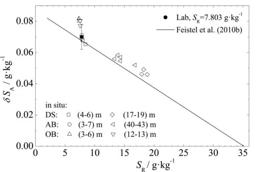
right column). Together with the laboratory estimate and the empirical parameterization (Eq. 1),δSAis shown in Fig. 3. Based on this consistent picture of the salinity anomaly

we evaluated the results from the sound speed sensor in view of the anomalous devi-ations.

In von Rohden et al. (2015) we documented the existence of certain inconsistencies

15

for speed of sound among the pure water calibrated time-of-flight sensors including the unit used here. These variations were an order of magnitude larger than the re-producibility and showed apparent trends with temperature and salinity. That means that an adequate calibration covering the large Baltic salinity range would be neces-sary for the comparison of direct sound speed readings. Such a calibration, however,

20

was not appropriate. Hence, a direct detection ofδw by a simple comparison of the

in situ values with sound speed derived from parallel CTD data using equations of state (assuming standard composition) was not applicable.

Instead, we related the differences of the actual sensor displays to the corresponding EOS-calculated values (w−wEOS)Balticwith the analogous differences (w−wEOS)Atlantic

25

which were calculated on the basis of laboratory records in two samples of diluted North Atlantic seawater (as a “substitute” for Standard Seawater):

(11)

OSD

12, 2565–2589, 2015

Seawater

Title Page

Tables Figures

◭ ◮

Back Close

Full Screen / Esc

Discussion

P

a

per

|

Discussion

P

a

per

|

Discussion

P

a

per

|

Discussion

P

a

per

|

The first of the reference samples is the one used for the laboratory estimate ofδw

withSP=7.765±0.007. The second is another Atlantic sample (NA I) diluted toSP=

16.66±0.03. Using these samples we classified the Baltic in situ measurements into

two groups by means of salinity in the sense that the two Atlantic reference samples can

be seen as representative of the twoSP ranges (7.3 to 8.4, and 13.3 to 18.8) sampled

5

during our Baltic Sea field trip. Tables 3 and 4 are accordingly separated into upper and lower parts. The sound speed differences (w−wEOS)Balticand (w−wEOS)Atlanticare

listed in Table 4 for both TEOS-10 and the Chen and Millero (1977) equation.

In principle, this proceeding is similar to a “local” recalibration of the sensor in sea-water at the two salinities. The approach of relating the Baltic field measurements with

10

the fixed Atlantic reference samples however implies that (w−wEOS) is basically

inde-pendent of salinity, at least within both defined salinity ranges. A possible dependence of the difference on pressure should be negligible due to the comparatively weak sensi-tivity of sound speed to pressure and the rather shallow sampling depths (<43 m). The comparatively strong temperature dependence of the reference differences (w−wEOS)

15

was considered by interpolation to the Baltic sample temperatures (CTD) using

poly-nomials. An example for the sample with SP=7.765 is given in Fig. 4. The data are

also listed in Table S2 in the Supplement. The results for the extracted sound speed anomalyδw are listed in Table 4 and plotted in Fig. 5. The courses of the differences

w−wEOSreflect the inaccuracy of both the sensor with respect to absolute values, and

20

the actual reference equation. However, due to the high sensor stability and resolution,

the uncertainty ofδwis expected to be much smaller than the uncertainties of each of

the two terms.

As a basic outcome we state that at least over the period of the field campaign (∼1

week) the sensor was stable. The data show a smooth course without strong salinity

25

dependence (Fig. 5). Especially theδwatSP≈8 reproduce well and independently of

(12)

OSD

12, 2565–2589, 2015

Seawater

Title Page

Tables Figures

◭ ◮

Back Close

Full Screen / Esc

Discussion

P

a

per

|

Discussion

P

a

per

|

Discussion

P

a

per

|

Discussion

P

a

per

|

Whereas the outputs of the equations apparently differ by≈0.05 m s−1(upper panel

of Fig. 5), the estimated sound speed anomaly δw is basically independent of the

equation used as a reference (lower panel), which was expected within the assump-tions and uncertainties of our approach. Note that the use of the Del Grosso and Mader (1974) equation as a reference would not be reasonable because of its validity limited

5

to oceanic salinities which do not include the brackish Baltic waters. Although a bit

lower, theδw atSP≈8 match the more accurate laboratory findings within the range

of uncertainties (Fig. 1) (discussion below). The high reproducibility of the measure-ments atSP≈8 also implies the validity of the results at higherSP (13.3 to 18.8), for

which no comparative experimental values are available, even though there are

some-10

what larger uncertainties due to the larger salinity error of our SP=16.66 reference

sample (NA I).

Contributions to the uncertainty of δw comprise the general stability of the sensor

(0.019 m s−1), represented by the reproducibility of calibration measurements in pure water, and the effect of conductivity (salinity), temperature, and pressure uncertainties

15

on EOS calculated sound speed (<0.04 m s−1). We assigned an additional contribution of 0.02 m s−1to the difference (w−wEOS)Atlantic (sensor display minus EOS calculated

sound speed), which accounts for the interpolation to the in situ measured tempera-tures (Fig. 4), and for the assumption of an insignificant salinity and pressure sensitivity of this difference. The limited validity of a vanishing salinity sensitivity might be indicated

20

by the somewhat suspiciousδw at theSP≈13.3 and SP≈18.8 with the largest

devi-ations to the reference salinity ofSP=16.66. The resulting overall uncertainty of the

sound speed anomalyu(δw) is given in Table 4.

3 Discussion

The results of the laboratory investigations represent the first experimental estimate of

25

the speed-of-sound anomaly caused by the anomalous salt composition in Baltic

(13)

OSD

12, 2565–2589, 2015

Seawater

Title Page

Tables Figures

◭ ◮

Back Close

Full Screen / Esc

Discussion

P

a

per

|

Discussion

P

a

per

|

Discussion

P

a

per

|

Discussion

P

a

per

|

the validity of the extractedδwwas supported by the consistency of the data measured

with three time-of-flight sensors from two manufacturers simultaneously, also at tem-peratures exceeding the natural range. The results show that with the high resolution and reproducibility of modern time-of-flight sensors, the anomaly effect can be resolved with comparison measurements.

5

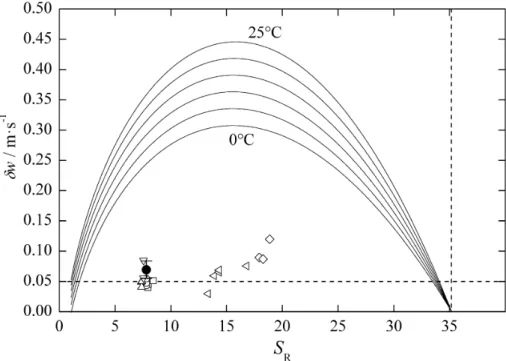
Feistel et al. (2010a) derived a Gibbs function for Baltic Seawater from Pitzer equa-tions using a numerical model (FREZCHEM) which simulates chemical and physical properties of seawater with variable solute composition. With this, the speed-of-sound deviation in Baltic water and seawater with the same electrical conductivity was pre-dicted under the presumption that the salt anomaly can be represented by additional

10

calcium carbonate coming from river water discharge. The results are shown in Fig. 25 in Feistel et al. (2010a). We reproduced the figure and added our measurement results to the model curves in Fig. 6. Obviously, within the uncertainty our results as a whole do not conform to the predictions. The good representation of our measurements by the line in Fig. 1 rather indicates comparability with the prediction following Millero’s

15

rule (see also Fig. 13 in Feistel et al., 2010a). From the field measurements in the Baltic Sea and from our separate study (von Rohden et al., 2015) we conclude that modern time-of-flight sensors are not (yet) applicable as a tool for the in situ detection of the salinity anomaly when calibrated in pure water only. To solve this, an extensive calibration in Standard Seawater covering the temperature and the large salinity range

20

of the Baltic Sea or significant improvements of the absolute sensor uncertainty are required.

With the in situ sensor application we showed that in the face of the above restrictions it is possible to give a reliable estimate of δw in a non-routine demonstration. In this

way we yielded adequate results for the salinity range ofSP≈7 to 19 and reproduced

25

well the laboratory results atSP=7.766 within the uncertainties.

(14)

OSD

12, 2565–2589, 2015

Seawater

Title Page

Tables Figures

◭ ◮

Back Close

Full Screen / Esc

Discussion

P

a

per

|

Discussion

P

a

per

|

Discussion

P

a

per

|

Discussion

P

a

per

|

is geographically, as well as temporally, and with respect to the solute composition, not homogeneous. That means that the anomalous salt component might be variable with

respective effects on the magnitude of sound speed deviations, dependent on the time

scales of the horizontal and the rather strongly salinity controlled diapycnal exchange processes. This might also be significant for the results of our in situ measurements.

5

Data availability

All relevant data are provided with Tables 2–4 in the manuscript and with two tables in the Supplement.

The Supplement related to this article is available online at doi:10.5194/osd-12-2565-2015-supplement.

10

Author contributions. C. von Rohden designed and carried out the laboratory experiments, supervised the offshore speed-of-sound measurements, evaluated the data, and wrote the manuscript. S. Weinreben prepared the field activities and carried out the on-board density and CTD measurements. F. Fehres contributed to the data evaluation and manuscript preparation.

Acknowledgement. This research was undertaken within the project EMRP ENV05. The 15

EMRP is jointly funded by the EMRP participating countries within EURAMET and the European Union.

Disclaimer. Any mention of commercial products within this study does not imply recom-mendation or endorsement by PTB.

20

References

(15)

OSD

12, 2565–2589, 2015

Seawater

Title Page

Tables Figures

◭ ◮

Back Close

Full Screen / Esc

Discussion

P

a

per

|

Discussion

P

a

per

|

Discussion

P

a

per

|

Discussion

P

a

per

|

Del Grosso, V. A.: New equation for the speed of sound in natural waters (with comparisons to other equations), J. Acoust. Soc. Am., 56, 1084–1091, doi:10.1121/1.1903388, 1974. Feistel, R., Marion, G. M., Pawlowicz, R., and Wright, D. G.: Thermophysical property

anoma-lies of Baltic seawater, Ocean Sci., 6, 949–981, doi:10.5194/os-6-949-2010, 2010a.

Feistel, R., Weinreben, S., Wolf, H., Seitz, S., Spitzer, P., Adel, B., Nausch, G., Schneider, B., 5

and Wright, D. G.: Density and Absolute Salinity of the Baltic Sea 2006–2009, Ocean Sci., 6, 3–24, doi:10.5194/os-6-3-2010, 2010b.

IOC, SCOR and IAPSO: The international thermodynamic equation of seawater-2010: Calcula-tion and use of thermodynamic properties, Intergovernmental Oceanographic Commission, Manuals and Guides No. 56, UNESCO (English), 196 pp., available at: http://www.teos-10. 10

org (last access: 21 October 2015), 2010.

McDougall, T. J., Jackett, D. R., Millero, F. J., Pawlowicz, R., and Barker, P. M.: A global al-gorithm for estimating Absolute Salinity, Ocean Sci., 8, 1123–1134, doi:10.5194/os-8-1123-2012, 2012.

Millero, F. J. and Kremling, K.: The densities of Baltic Sea waters, Deep-Sea Res., 23, 1129– 15

1138, 1976.

Millero, F. J., Waters, J., Woosley, R., Huang, F., and Chanson, M.: The effect of com-position on the density of Indian Ocean waters, Deep-Sea Res. Pt. I, 55, 460–470, doi:10.1016/j.dsr.2008.01.006, 2008.

Perkin, R. G. and Lewis, E.: The Practical Salinity Scale 1978: Fitting the data, IEEE Journal of 20

Ocean. Engin., Deep-Sea Res. Pt. I, 5, 9–16, doi:10.1016/0198-0149(81)90002-9, 1980. Von Rohden, C., Fehres, F., and S. Rudtsch, S.: Capability of pure water calibrated time-of-flight

(16)

OSD

12, 2565–2589, 2015

Seawater

Title Page

Tables Figures

◭ ◮

Back Close

Full Screen / Esc

Discussion

P

a

per

|

Discussion

P

a

per

|

Discussion

P

a

per

|

Discussion

P

a

per

|

Table 1.Sensor specifications. The response times basically reflect the time of flight of sound pulses. The reproducibility corresponds to the standard uncertainty for measurements in pure water in our experimental setup over a period of one (AML) and two years (VP), respectively (von Rohden et al., 2015).

AML SVX VP, VP OEM

acoustic pathlength /mm 68 200

response time /µs _∼47 _∼140

time resolution /ns _∼0.02 0.01

practical resolutionw/m s−1 0.001 0.001 reproducibility /m s−1

(17)

OSD

12, 2565–2589, 2015

Seawater

Title Page

Tables Figures

◭ ◮

Back Close

Full Screen / Esc

Discussion

P

a

per

|

Discussion

P

a

per

|

Discussion

P

a

per

|

Discussion

P

a

per

|

Table 2.Salinity estimates for the samples used, and salinity differences related to the compo-sition anomaly for the Baltic seawater sample, including standard uncertainties.

Salinity (g kg−1

) Baltic North Atlantic

diluted original

S_P/PSU 7.766±0.007 7.765±0.007 36.208±0.01

S_A,cond(assum. standard comp.) 7.803_±0.007 7.801_±0.007 36.379_±0.01 S_A,dens(from measured density) 7.870_±0.006 36.381_±0.006 Meas. diff.δS_A,m=S_A,dens–S_A,cond 0.067_±0.009

(18)

OSD

12, 2565–2589, 2015

Seawater

Title Page

Tables Figures

◭ ◮

Back Close

Full Screen / Esc

Discussion

P

a

per

|

Discussion

P

a

per

|

Discussion

P

a

per

|

Discussion

P

a

per

|

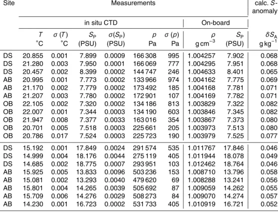
Table 3.CTD data (averages of 2 min recordings at constant depths) at three sites in the Baltic Sea (see Fig. 2) in August 2014 including standard deviations;p=hydrostatic plus air pressure. Three right columns: on-board density and salinity measurements as averages of two samples taken in parallel to the CTD measurements; calculated salinity anomalyδS_Abased on on-board measurements.

Site Measurements calc.S

-anomaly

in situ CTD On-board

T σ(T) SP σ(SP) p σ(p) ρ SP δSA

◦_C ◦_C _(PSU) _(PSU) _Pa _Pa _{g cm}−3

(PSU) g kg−1

DS 20.855 0.001 7.899 0.0009 166 308 995 1.004257 7.902 0.068 DS 21.280 0.003 7.950 0.0001 166 069 777 1.004295 7.951 0.068 DS 20.457 0.002 8.399 0.0002 144 747 246 1.004633 8.401 0.065 AB 20.995 0.001 7.773 0.0002 133 966 974 1.004162 7.775 0.069 AB 21.170 0.002 7.779 0.0002 173 492 185 1.004168 7.781 0.071 AB 21.207 0.003 7.780 0.0002 172 901 107 1.004169 7.782 0.071 OB 22.105 0.002 7.320 0.0002 134 186 813 1.003829 7.322 0.082 OB 22.007 0.001 7.344 0.0003 134 190 603 1.003846 7.345 0.082 OB 21.947 0.008 7.377 0.0033 163 016 354 1.003867 7.373 0.080 OB 20.701 0.005 7.518 0.0003 225 661 205 1.003973 7.513 0.080 OB 20.786 0.017 7.524 0.0003 225 723 190 1.003979 7.525 0.077

(19)

OSD

12, 2565–2589, 2015

Seawater

Title Page

Tables Figures

◭ ◮

Back Close

Full Screen / Esc

Discussion

P

a

per

|

Discussion

P

a

per

|

Discussion

P

a

per

|

Discussion

P

a

per

|

Table 4.Speed of sound measured with the time-of-flight sensor in the Baltic Sea (in m s−1);w -differences (measured minus calculated) using TEOS-10 and Chen and Millero (1977) for the Baltic in-situ measurements, and for the laboratory measurements in samples of natural Atlantic seawater withS_P=7.765 (upper part of table) andS_P=16.66 (lower part). The di_fferences in the Atlantic samples were previously interpolated to the Baltic in situ temperatures. δw are the respective estimates of the sound speed anomaly according to Eq. (2). The uncertainty estimateu(δw) (right column) is virtually the same for both reference equations. The data are in the same order as in Table 3.

Site measured sound speed rel. to TEOS-10 rel. to Chen and Millero (1977)

Baltic Atlantic Baltic Atlantic

w σ(w) w−wTEOS w−wTEOS δω w−wCM77 w−wCM77 δω u(δω)

DS 1493.982 0.004 0.073 0.033 0.040 0.026 −0.013 0.039 0.033

DS 1495.284 0.005 0.081 0.036 0.045 0.032 −0.012 0.044 0.034

DS 1493.338 0.005 0.081 0.030 0.051 0.034 −0.014 0.048 0.033

AB 1494.203 0.005 0.077 0.034 0.043 0.030 −0.013 0.043 0.033

AB 1494.792 0.005 0.082 0.036 0.047 0.034 −0.012 0.047 0.033

AB 1494.907 0.009 0.090 0.036 0.055 0.042 −0.012 0.054 0.035

OB 1496.914 0.006 0.090 0.042 0.049 0.041 −0.010 0.051 0.033

OB 1496.653 0.005 0.082 0.041 0.041 0.033 −0.010 0.043 0.033

OB 1496.573 0.009 0.090 0.041 0.050 0.041 −0.010 0.052 0.041

OB 1493.218 0.010 0.088 0.032 0.056 0.041 −0.014 0.055 0.037

OB 1493.506 0.017 0.118 0.033 0.085 0.071 −0.013 0.084 0.063

DS 1487.770 0.005 0.074 −0.015 0.089 0.031 −0.053 0.084 0.048

DS 1487.476 0.007 0.070 −0.017 0.087 0.026 −0.054 0.081 0.050

DS 1487.180 0.010 0.099 −0.021 0.120 0.056 −0.057 0.113 0.049

AB 1485.888 0.013 0.053 −0.006 0.059 0.011 −0.047 0.059 0.053

AB 1482.389 0.008 0.013 −0.016 0.030 −0.021 −0.054 0.033 0.049

AB 1485.985 0.005 0.057 ₋0.007 0.065 0.015 ₋0.048 0.064 0.050

AB 1485.703 0.015 0.060 −0.009 0.069 0.018 −0.049 0.067 0.053

(20)

OSD

12, 2565–2589, 2015

Seawater

Title Page

Tables Figures

◭ ◮

Back Close

Full Screen / Esc

Discussion

P

a

per

|

Discussion

P

a

per

|

Discussion

P

a

per

|

Discussion

P

a

per

|

Figure 1.Speed-of-sound differences associated with the salinity anomaly for Baltic seawater atS_P=7.766. Symbols: measured differences from the Baltic and the diluted Atlantic sample (NA II) with virtually the same S_P. Uncertainty bars are exemplary given at 4◦_{C. Line:} _δw

(21)

OSD

12, 2565–2589, 2015

Seawater

Title Page

Tables Figures

◭ ◮

Back Close

Full Screen / Esc

Discussion

P

a

per

|

Discussion

P

a

per

|

Discussion

P

a

per

|

Discussion

P

a

per

|

(22)

OSD

12, 2565–2589, 2015

Seawater

Title Page

Tables Figures

◭ ◮

Back Close

Full Screen / Esc

Discussion

P

a

per

|

Discussion

P

a

per

|

Discussion

P

a

per

|

Discussion

P

a

per

|

(23)

OSD

12, 2565–2589, 2015

Seawater

Title Page

Tables Figures

◭ ◮

Back Close

Full Screen / Esc

Discussion

P

a

per

|

Discussion

P

a

per

|

Discussion

P

a

per

|

Discussion

P

a

per

|

(24)

OSD

12, 2565–2589, 2015

Seawater

Title Page

Tables Figures

◭ ◮

Back Close

Full Screen / Esc

Discussion

P

a

per

|

Discussion

P

a

per

|

Discussion

P

a

per

|

Discussion

P

a

per

|

(25)

OSD

12, 2565–2589, 2015

Seawater

Title Page

Tables Figures

◭ ◮

Back Close

Full Screen / Esc

Discussion

P

a

per

|

Discussion

P

a

per

|

Discussion

P

a

per

|

Discussion

P

a

per

|

Figure 6. Experimental data for sound speed anomaly δw in Baltic seawater (symbols) in comparison to model results (lines, reproduced from Fig. 25 in Feistel et al., 2010a) at at-mospheric pressure. Filled symbol: average of laboratory measurements in a sample with SR=7.803 g kg−

1