MODELING AND FORECASTING THE
GROSS ENROLLMENT RATIO IN ROMANIAN PRIMARY SCHOOL
MARINOIU CRISTIAN
ASSOC. PROF.PH.D., PETROLEUM-
GAS UNIVERSITY OF PLOIEŞTI, ROMANIA
e-mail:[email protected]
Abstract
The gross enrollment ratio in primary school is one of the basic indicators used in order to evaluate the proposed objectives of the educational system. Knowing its evolution allows a more rigorous substantiation of the strategies and of the human resources politicsnot only from the educational field but also from the economic one. In this paper we propose an econometric model in order to describe the gross enrollment ratio in Romanian primary school and we achieve its prediction for the next years, having as a guide the Box -Jenkins’s methodology. The obtained results indicate the continuousdecrease of this rate for the next years.
Key-words: time series, forecast, ARIMA, gross enrollment ratio
Classification JEL: C50, I21
1.
Introduction
The evaluation of the working condition of an educational system is achieved on the basis of a set of indicators which reflect the fundamental aspects of such a system: the educational context, the educational resources, the access and the participation in education and the results of education. The access and the participation in education are quantified through specific indicators: the gross scholar enrollment ratio, the net scholar enrollment ratio, the school life expectancy and so on.
The primary scholar gross enrollment ratio (GER) represents the percentage of pupils included in primary education, regardless of their age, relative to the total population from the official age-group which corresponds to the primary educational system [1]. This percentage can exceed 100% because we can include into the primary school pupils who are outside the official limits of age (either because they were too early or too late registred in school, or because of dropping school).
GER is an important indicator in the process of evaluating the conditions in the educational system from a country or from a region. Predicting its evolution can be useful in order to implement the medium and long term policies and strategies from the human resources field and, specially, from the educational system.
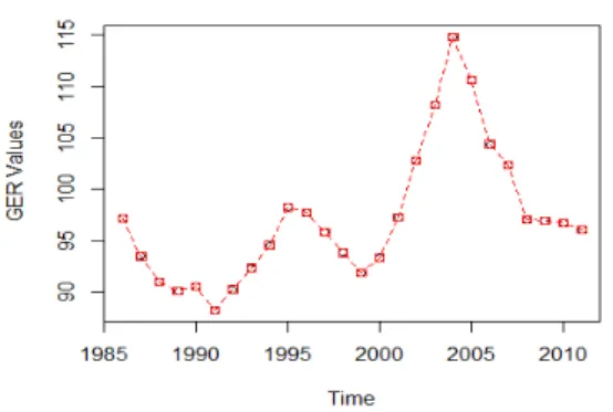
The study presented in this paper is based on the annual values of GER for Romania, which correspond to the period 1986-2011, presented in [2]. The objective is to build an econometricmodel starting from these data, to validate it and to make predictions about the GER evolution for the next years.
2.
The GER time series
The GER values observed annually form a time series and may be considered as realizations of a random process
y
t.
The time series is graphically represented in figure 1 and it has the mean equal to 97.16584 and theSource: made by the author in R using data from [2]
The graph does not present clues that suggest an unstable variance. At the same time some increases and decreases are obvious for long periods of time (for example the periods 2000-2005 and 2005-2011), which suggest the fact that the series is not stationary. In order to verify this hypothesis we applied the ADF (Augmented –Dickey-Fuller) and KPSS (Kwiatkowski-Philips-Schimdt-Shin) tests [3], used in order to detect the non-stationarity, the level of significance being fixed to 0.05. The p-values of the two tests are represented in table 1.
Table 1.The results of the ADF and KPSS tests
Test p-values
Augmented –Dickey-Fuller(ADF) 0.237
Kwiatkowski-Philips-Schimdt-Sh in(KPSS) 0.02323
Source: made by the author with results obtained in R
The null hypothesis of ADF test is that the series is not stationary, while the null hypothesis o f KPSS test is that the series is stationary. In the case of ADF test we have 0.237>0.05 so we cannot reject the hypothesis that the series is not stationary. In the case of KPSS test we have 0.02323<0.05 so we reject the hypothesis that the series is stationary.
As a consequence, taking into account all these observations, we arrive at the conclusion that the series is not stationary.
3. The selection of the best model
Due to the fact that the GER time seris is not stationary, we will try to transform it into a stationary time series. We may often obtain a stationary time series
z
tfrom a non-stationary time seriesy
t through a transformation suchas:
z
ty
ty
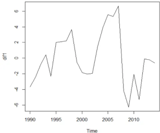
t 1, named the difference of first order [4 ]. The difference of first order of the time series GER, namedFigure 2. The time series difference of first order (dif1) Source: made by the author in R
The aspect of the time series dif1 suggests that the series of the differenced data seems to be stationary. By applying the KPSS test to the time series dif1 we obtain the p-value equal to 0.1. Because 0.1>0.05 we cannot reject the hypothesis that the time series of the differencies of first order (dif1) is stationary.
The choice of the best model for the GER time series can be done automatically by using the special functions of different software packages or „manually” by selecting from many candidate models the model which has the best values for certain indicators (for example the smallest values for the AIC or BIC statistics). In order to select the most suitable model we prefered to use the automatic variant based on the implementation of the function auto.arima()[5] from the library forecast [6] of the software package R .
The selected model on the basis of this function is , in this case, ARIMA(1,1,0) with drift, the results being as it follows:
Coefficients: ar1 drift 0.5213 -0.2103 s.e. 0.1716 1.1560
sigma^2 estimated as 8.253: log likelihood=-59.04 AIC=124.09 AICc=125.23 BIC=127.75
As a consequence, the proposed model is:
y
ty
t 10
.
5213
(
y
t 1y
t 2)
0
.
2103
4.
The validation of the selected model
The validation of the selected model involves checking the following conditions: The residuals of the model are not correlated;
The residuals of the model are normally distributed with mean 0 and constant variance.
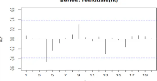
The graphical representation of residuals (fig. 4) suggests that errors are not correlated (we cannot observe a certain pattern of these residuals ).
Figure 5.The correlogram of residuals. The 95% significance bounds aremarked by dashed lines. Source: made by the author using the functions from R.
The Ljung-Box test [7]-[8] is one of the tests through which we can verify the null hypothesis: H0: residuals are not correlated
against
Ha: residuals are correlated.
The results ofusing of this test at the level of significance 0.05 are represented in figure 6. We may observe that all the p-values which correspond to the first 10 lags are superior to 0.05 (value marked in the figure by a dashed line), which signify that we accept the hypothesis that residuals are not correlated.
Consequently, the results of Ljung-Box test confirm the fact that residuals are not correlated.
Figure 6. In this picture, thep-values of the test Ljung- Box for the first 10 lags are marked with circles . The dashed line emphasizes the value 0.05 under which the null hypothesis is rejected.
Source: made by the author in R
In order to verify the normality of residuals, we will analize the hystogram of residuals, the graph qq plot of residuals and the results of the Shapiro-Wilk test [9].
Figure 7 . Left: the histogram of residuals with overlaid normal curve. Right: the graph qqplot of residuals .
Source: made by the author using the functions from R (in order to realize the histogram we used the function built by Avril Coghlan [10])
Using the Shapiro-Wilk test we verify the null hypothesis H0: residuals are normally distributed
against
Ha: residuals are not normally distributed.
The p-value is equal to 0.1807. Because 0.1807>0.05 (level of significance) we cannot reject the null hypothesis H0. Taking into account the histogram of residuals, the graph qqplot of residuals and the results of the test Shapiro-Wilk we conclude that residuals are normally distributed.
Because the residuals of the model obtained ARIMA(1,1,0) are not correlated and normally distributed we conclude that the model obtained is valid.
5. The forecast of the GER time series values
The fact that the model ARIMA (1,1,0) is valid allows us to proceed to the next step, predicting the GER time series values for the next years and building prediction intervals for these forecasts . The results presented in Table 4 are obtained using the function forecast from R.
Table 4. Forecast values and their 80% (Lo 80, Hi 80) and 90% (Lo 95, Hi 95) prediction intervals
Year Forecast Lo 80 Hi 80 Lo 95 Hi 95
2015 95.68132 91.99957 99.36307 90.05057 101.3121 2016 95.35964 88.65700 102.06227 85.10883 105.6104 2017 95.09130 85.68373 104.49887 80.70367 109.4789 2018 94.85077 83.05095 106.65059 76.80450 112.8970 2019 94.62473 80.69938 108.55008 73.32775 115.9217 2020 94.40625 78.57241 110.24009 70.19048 118.6220 2021 94.19171 76.62401 111.75941 67.32422 121.0592 2022 93.97922 74.81870 113.13974 64.67574 123.2827 2023 93.76780 73.12963 114.40597 62.20445 125.3312 2024 93.55694 71.53642 115.57746 59.87947 127.2344
Source: Results obtained by the author using functions from R
Figure 8 . The graphof the GER time series values,the forecasts for the years 2015-2024 (the line included in the shaded area) as well as the 80% (the dark shaded area) and the 95% prediction intervals (the light shaded area).
Source: made by the author using the functions from R
6. Conclusions
This paper introduced an econometric model for the gross enrollment ratio in Romanian primary school (GER), having as a guide the methodology Box-Jenkins. In order to process the data and to analyze the results we used the software package R.The predictions realized on the basis of the model obtained show a continuous decrease of GER values in the next years. The results obtained can be a good starting point for any study which has as a theme the establishement of personnel policies in the educational system and the preparation of the Romanian labour force.
7.
Bibliography
[1] Cezar Bîrzea ş.a, Sistemul naţional de indicatori pentru educaţie-manual de utilizare, Bucharest, 2005- developed by Proiectul pentru învăţamânt rural: http://www.edu.ro/index.php/articles/c148/
[2]***http://data.worldbank.org/country/romania [3]***https://www.otexts.org/fpp/8/1
[4]***http://www.itl.nist.gov/div898/handbook/pmc/section4/pmc442.htm
[5]***http://www.inside-r.org/packages/cran/forecast/docs/auto.arima
[6]***http://www.jstatsoft.org/v27/i03/paper
[7]***http://stat.ethz.ch/R-manual/R-patched/library/stats/html/box.test.html
[8]***http://a-little-book-of-r-for-time-series.readthedocs.org/en/latest/src/timeseries.html
[9]***http://www.answers.com/topic/shapiro-wilk-test
[10]***http://altons.github.io/r/2013/05/12/arima-models-in-a-nutshell/