Apparent oxygen utilization rates calculated from tritium and helium-3 profiles at the Bermuda Atlantic Time-series Study site

(1)

BGD

8, 9977–10015, 2011

Apparent oxygen utilization rates

R. H. R. Stanley et al.

Title Page

Abstract Introduction

Conclusions References

Tables Figures

◭ ◮

Back Close

Full Screen / Esc

Printer-friendly Version Interactive Discussion

Discussion

P

a

per

|

Dis

cussion

P

a

per

|

Discussion

P

a

per

|

Discussio

n

P

a

per

|

Biogeosciences Discuss., 8, 9977–10015, 2011 www.biogeosciences-discuss.net/8/9977/2011/ doi:10.5194/bgd-8-9977-2011

Biogeosciences Discussions

This discussion paper is/has been under review for the journal Biogeosciences (BG). Please refer to the corresponding final paper in BG if available.

Apparent oxygen utilization rates

calculated from tritium and helium-3

profiles at the Bermuda Atlantic

Time-series Study site

R. H. R. Stanley, S. C. Doney, W. J. Jenkins, and D. E. Lott, III

Marine Chemistry and Geochemistry Department, Woods Hole Oceanographic Institution, Woods Hole MA 02543, USA

Received: 14 September 2011 – Accepted: 15 September 2011 – Published: 11 October 2011

Correspondence to: R. H. R. Stanley (rstanley@whoi.edu)

(2)

BGD

8, 9977–10015, 2011

Title Page

Tables Figures

◭ ◮

Back Close

Full Screen / Esc

Discussion

P

a

per

|

Dis

cussion

P

a

per

|

Discussion

P

a

per

|

Discussio

n

P

a

per

|

Abstract

We present three years of Apparent Oxygen Utilization Rates (AOUR) estimated from oxygen and tracer data collected over the ocean thermocline at monthly resolution be-tween 2003 and 2006 at the Bermuda Atlantic Time-series Study (BATS) site. We estimate water ages by calculating a transit time distribution from tritium and helium-3

5

data. The vertically integrated AOUR over the upper 500 m, which is a regional esti-mate of export, during the three years is 3.1±0.5 mol O2m−2yr−1. This is comparable

to previous AOUR-based estimates of export production at the BATS site but is several times larger than export estimates derived from sediment traps or 234Th fluxes. We compare AOUR determined in this study to AOUR measured in the 1980s and show

10

AOUR is significantly greater today than decades earlier because of changes in AOU, rather than changes in ventilation rates. The changes in AOU may be a methodological artefact associated with problems with early oxygen measurements.

1 Introduction

Recently, a number of papers have been published in the scientific literature

suggest-15

ing that the oxygen content in the ocean is decreasing (Keeling et al., 2010; Deutsch et al., 2011). This decrease, both predicted in models (Bopp et al., 2002; Matear and Hirst, 2003; Plattner et al., 2001) and seen in data (Stramma et al., 2008; Whitney et al., 2007; Stramma et al., 2010), is due to the ocean becoming warmer and more stratified. Deoxygenation is likely to a_ffect the elemental cycles of many biogeochemically

rele-20

vant species (C, N, P, Fe) (Codispoti et al., 2001; Wallmann, 2003). Additionally, most organisms are sensitive to oxygen levels, with a nonlinear sensitivity at low oxygen lev-els, suggesting that large-scale negative ecosystem consequences to deoxygenation may occur (Vaquer-Sunyer and Duarte, 2008). Documenting and understanding the nature of the trend in oceanic oxygen is important both from the viewpoint of global

25

(3)

BGD

8, 9977–10015, 2011

Title Page

Tables Figures

◭ ◮

Back Close

Full Screen / Esc

Discussion

P

a

per

|

Dis

cussion

P

a

per

|

Discussion

P

a

per

|

Discussio

n

P

a

per

|

cycling of carbon and other elements. Time-series data of oxygen records are vital for addressing this question. Futhermore, diagnosing the magnitude of oxygen sinks within the water column is key to developing our understanding of the relevant biogeo-chemical dynamics.

One method for quantifying the biological oxygen sinks is to determine Apparent

5

Oxygen Utilization Rates (AOUR), a geochemical tracer-based metric of export pro-duction which integrates over a large geographic area. AOUR are calculated by com-bining oxygen utilization data with a natural “clock“, typically a tracer that yields infor-mation on the age of the water mass. Geochemical clocks for dating water include tritium/helium-3 (T/3He) (e.g. Jenkins, 1977, 1980, 1988, 1998), chlorofluorocarbons

10

(CFC) (e.g. Doney and Bullister, 1992; Smethie and Fine, 2001), and for the upper few hundred meters7Be (Kadko, 2009). Tritium decays with a 12.31 year half-life to3He, a stable, inert isotope (MacMahon, 2006). The primary source of tritium to the contem-porary ocean is from tritium released by the atmospheric thermonuclear bomb tests in the 1960s. Thus, T/3He is most useful for dating water that has been at the surface

15

within the last 50 years. When the water is at the surface, excess3He, i.e. 3He con-centration above the solubility value, is almost completely lost due to gas exchange. As water is sequestered from the atmosphere and ages, excess 3He builds up and tritium decreases. In theory, the radioactive decay equation could be used to estimate ventilation ages. In practice, however, mixing complicates matters and thus simple box

20

models have been used in order to estimate ventilation time scales (Doney and Jenk-ins, 1988; JenkJenk-ins, 1980). Here we apply both the box model approach and a newer, more sophisticated approach, namely using Transit Time Distributions (TTD) (Waugh et al., 2003; Khatiwala et al., 2009) to calculate ventilation ages.

The apparent oxygen utilization (AOU) – the di_fference between equilibrium O₂and

25

(4)

BGD

8, 9977–10015, 2011

Title Page

Tables Figures

◭ ◮

Back Close

Full Screen / Esc

Discussion

P

a

per

|

Dis

cussion

P

a

per

|

Discussion

P

a

per

|

Discussio

n

P

a

per

|

euphotic zone. However, the AOUR of a water parcel represents the time averaged oxygen consumption rate along an isopycnal path from when the water was first sub-ducted to when it arrived at a given site. Thus, the depth-integrated AOUR is not simply a measure of local export but rather is a projection of geographic and horizon-tally distributed processes working on individual isopycnal layers and hence represents

5

a regional view of export flux. This key point is discussed in more detail in Sect. 4.1. In this paper, we present AOUR as determined from T and3He ages, calculated us-ing transit time distributions, at the Bermuda Atlantic Time-series Study (BATS) site, a typical subtropical oligotrophic gyre location. BATS is an ideal location for this work as there is a wealth of geochemical data for comparison. A time-series of many

biogeo-10

chemical parameters has been measured at BATS since 1988 (Michaels and Knap, 1996; Steinberg et al., 2001). Tritium and 3He have been measured at BATS and nearby Station S at various times since the mid-1970s (Jenkins, 1977, 1998, 1980, 1988). Export production has been calculated at BATS, specifically, and in the Sar-gasso Sea in general, from the AOUR method (Garcia et al., 1998; Hansell and

Carl-15

son, 2001; Jenkins, 1980), from sediment traps (Lomas et al., 2010; Stanley et al., 2004; Steinberg et al., 2001), and from 234Th disequilibrium (Buesseler et al., 2008; Maiti et al., 2010).

Here, we present T and 3He data collected at roughly monthly resolution between 2003 and 2006. In Sect. 2, we describe the data collection, the transit time distribution

20

approach, and the method for calculating AOUR. In Sect. 3, we present the the venti-lation ages, AOU, and AOUR at the BATS site as well as the depth-integrated AOUR as a measure of export flux. In Sect. 4, we discuss the implications of local versus regional export approaches, the depth and spatial distribution of AOUR, a comparison to other estimates of export at BATS, and a comparison to AOUR at BATS in the 1970s

25

(5)

BGD

8, 9977–10015, 2011

Title Page

Tables Figures

◭ ◮

Back Close

Full Screen / Esc

Discussion

P

a

per

|

Dis

cussion

P

a

per

|

Discussion

P

a

per

|

Discussio

n

P

a

per

|

2 Methods

2.1 Data collection

Samples were collected at the Bermuda Atlantic Time-series Study (BATS) site (31.7◦_{N, 64.2}◦_{W) on core BATS cruises at approximately monthly resolution between} April 2003 and April 2006. The BATS site is representative of the oligotrophic

subtrop-5

ical North Atlantic and a wealth of biogeochemical data has been collected there as part of the time-series study located there (Steinberg et al., 2001).

Tritium samples were collected from Niskin bottles by gravity feeding into 500 mL or 950 mL argon-filled flint glass bottles – water samples at depths<400 m were typ-ically in 500 mL bottles while the deeper samples were in the 950 mL bottles. The

10

bottles were filled with seawater to the “shoulder”, leaving approximately 50 to 100 mL of Ar “blanket” present in order to minimize exchange with atmospheric water vapour. Samples were collected at the surface, 50 m, 100 m, 140 m, 200 m, 250 m, 300 m, and 400 m every month. Additionally, approximately every 3 months, samples were col-lected at an additional 22 depths between 500 m and 4200 m.

15

The bottles were returned to the Isotope Geochemistry Facility (IGF) at Woods Hole Oceanographic Institution (WHOI) where, on a high-vacuum line, the samples were transferred using negative pressure under an Ar “blanket” to approximately half-fill 200 mL or 500 mL pre-evacuated aluminosilicate glass bulbs. The water was then de-gassed by alternating six 15 min periods of shaking with six 4 min periods of pumping.

20

The bulbs were flame-sealed and stored in the basement of the laboratory building to shield them from cosmogenic production of3He during the decay period. For more details on the degassing procedure, see Lott and Jenkins (1998).

After waiting at least six months for ingrowth of 3He from tritium decay, the sam-ples were analysed on a purposefully constructed, branch tube, statically operated,

25

(6)

BGD

8, 9977–10015, 2011

Title Page

Tables Figures

◭ ◮

Back Close

Full Screen / Esc

Discussion

P

a

per

|

Dis

cussion

P

a

per

|

Discussion

P

a

per

|

Discussio

n

P

a

per

|

equation, the storage time and the amount of3He measured. Tritium results are ex-pressed in Tritium Units (TU), where

TU₌ Tritium atoms Hydrogen atoms×10

18 ₍₁₎

Helium-3 samples were collected from the same Niskin bottles by gravity feeding through tygon tubing into valved 90 mL stainless steel sample cylinders. We extracted

5

gases from the water stored in the cylinders into _∼30 ml aluminosilicate glass bulbs at an on-shore laboratory within 24 h of sampling (Lott and Jenkins, 1998). We then brought the bulbs to the IGF at WHOI, where we attached the samples to a dual mass spectrometric system and analysed them for3He, as well as a suite of noble gases (He, Ne, Ar, Kr, and Xe) according to Stanley et al. (2009). In particular,3He was measured

10

on a purposefully constructed magnetic sector mass spectrometer, similar in design to that used to measure tritium.

Oxygen concentrations were measured on samples from the same Niskin bottles by Winkler titration according to standard BATS procedures (Knap et al., 1997).

2.2 Calculation of age of water

15

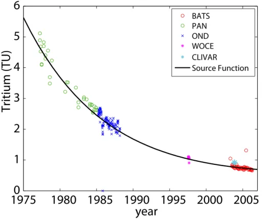
The mean age of the water was calculated from the tritium and3He data using a transit time distribution (TTD) approach (Waugh et al., 2003). In order to do so, we first created an updated surface water tritium source function for BATS. We used the Dreisigacker and Roether (1978) source function in a slightly corrected version until 1969 (Doney and Jenkins, 1988). From 1969 onwards, we determined a source function by fitting

20

an exponential function to surface tritium data collected near the BATS site as part of Panulirus (1975 to 1984) (Jenkins, 1998), OND (1982 to 1986) (Jenkins, 1998), WOCE A22 (1997) (http://cchdo.ucsd.edu/), CLIVAR Repeat Hydrography A22 (2003) (http://cchdo.ucsd.edu/), and this project (2003–2006) (Fig. 1). The best fit function for t >1969 was

25

(7)

BGD

8, 9977–10015, 2011

Title Page

Tables Figures

◭ ◮

Back Close

Full Screen / Esc

Discussion

P

a

per

|

Dis

cussion

P

a

per

|

Discussion

P

a

per

|

Discussio

n

P

a

per

|

where SF is the surface tritium concentration, in TU, for fractional year t. We realize this may be an oversimplification since the water collected at depth at BATS (i.e. our samples) did not necessarily surface at BATS itself. There are latitudinal gradients in source function but the differences are relatively small, as long as the water surfaces within the subtropical North Atlantic (Jenkins, 1988; Doney and Jenkins, 1988). In

5

Sect. 4.4, we examine the sensitivity of the results to variations in the source function. The TTD approach rests on the fact that there is not a single pathway that a wa-ter parcel takes between the surface ocean and a given location and depth. Rather, the di_fferent water molecules in the parcel have come from di_fferent locations, all with different transit times. Thus, instead of assigning a single age to a water parcel, a

prob-10

ability distribution of ages, often of the form of an inverse Gaussian, is used to describe the age of the water parcel. We use the probability distribution and the tritium source function to determine values of T and3He associated with di_fferent possible mean ages for water collected a given depth and time. We then use our data – the actual T and

3

He measured in a given water sample we collected at BATS – to determine which of

15

these possible mean ages is most suitable for that water parcel. Hence, we determine a mean age for each sample and use this mean age, in concert with the oxygen data, to calculate an AOUR for each sample.

Mathematically, the probability distribution, G, we use to describe the continuum of ages,t, is the Greens function (Eq. 16 from Waugh et al., 2003):

20

G₌ s

Γ3

4π_∆2_t3× exp (−Γ×

(t₋_Γ)2

4_∆2_t ) (3)

whereΓ is defined as the first moment of G and reflects the mean age of the water (Eq. 4 from Waugh et al., 2003):

Γ =

Z∞

0

(8)

BGD

8, 9977–10015, 2011

Title Page

Tables Figures

◭ ◮

Back Close

Full Screen / Esc

Discussion

P

a

per

|

Dis

cussion

P

a

per

|

Discussion

P

a

per

|

Discussio

n

P

a

per

|

and∆is defined as the width ofGand represents the width of the distribution, i.e. the spread of ages around the mean (Eq. 5 from Waugh et al., 2003):

∆2=1

2 Z∞

0

(t₋_Γ)2G(t)d t (5)

The ratio of_Γ/_∆is analogous to the Peclet number.

5

First, we calculate the probability distributions, G, as a function of age, t (ranging from 0 to 200 years), according to Eq. 3 for a series of mean age values,_Γfrom 1 to 100 years. For our base case results, we use the common assumption that_Γ/_∆ (Hall et al., 2004; Waugh et al., 2004, 2006). Additionally, we use the3He and T data from this study as well as from previous studies near BATS and Station S to constrain the

10

possible range of_Γ/_∆ to be between 0.8 and 1.2, and we perform a sensitivity study for this range (see Sect. 4.4 for more details).

After we calculate the probability distributionGwith a range of_Γ from 1 to 100 and a given_Γ/_∆, we then convolve G, (Eq. 3), with the source function (Eq. 2), which we have decay corrected to the time of sampling, in order to produce a pair of values of T

15

and3He for each_Γ. This gives us a lookup table of T and3He values that correspond to possible mean ages. Finally, we compare the 3He concentration we measured in the BATS samples to the3He values calculated for the di_fferent possible_Γs in order to determine_Γ_best, the mean age that most appropriately represents that sample. In this manuscript, we refer to this_Γ_best as τ. Hence, τ represents the best estimate of the

20

mean age of the water parcel. In theory, one could use either the3He or the tritium data to determineτ; in practice, we found that the3He data provided a more precise and robust determination, especially on shorter time scales. The errors onτ(grey error bars in Fig. 3) are calculated by determining the range of values on the lookup table corresponding to the measurement uncertainty window of the3He analyses.

25

(9)

BGD

8, 9977–10015, 2011

Title Page

Tables Figures

◭ ◮

Back Close

Full Screen / Esc

Discussion

P

a

per

|

Dis

cussion

P

a

per

|

Discussion

P

a

per

|

Discussio

n

P

a

per

|

2.3 Calculation of apparent oxygen utilization rates

Apparent Oxygen Utilization (AOU) is defined as the di_fference between the equilib-rium, or solubility value, of oxygen and the measured concentration:

AOU₌[O₂]_eq−[O2]meas (6)

where [O₂]_eqis the solubility value for the temperature and salinity of the water sample

5

according to Garcia and Gordon (1992) and [O₂]_measis the measured oxygen concen-tration of the sample. AOU is a measure of how much oxygen has been consumed, assuming that the oxygen concentration was at equilibrium with the atmosphere when the water was at the surface. The surface water probably was not at 100 % saturation because of bubble processes, which increase the degree of saturation, and the e_ffects

10

of atmospheric pressure, which in the water formation regions often decrease the de-gree of saturation. Still, the water was probably within a few percent of saturation (see Sect. 4.4 for a more precise treatment of this uncertainty).

The Apparent Oxygen Utilization Rate (AOUR), the rate at which oxygen is con-sumed, is given by

15

AOUR=AOU_τ (7)

Since the main pathway for oxygen consumption is organic matter respiration, the depth-integrated AOUR is a measure of the export production flux. However, the AOUR-derived export flux is nonlocal, i.e. it averages over the entire trajectory of the water parcels at each depth, and thus, given the shape of the subtropical gyre, is biased

20

(10)

BGD

8, 9977–10015, 2011

Title Page

Tables Figures

◭ ◮

Back Close

Full Screen / Esc

Discussion

P

a

per

|

Dis

cussion

P

a

per

|

Discussion

P

a

per

|

Discussio

n

P

a

per

|

3 Results

3.1 Helium and tritium data

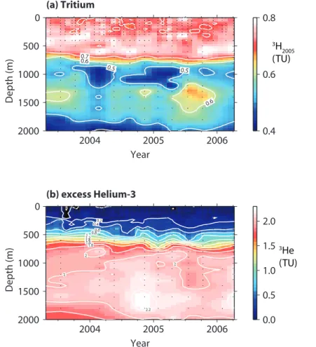
We present the T and excess 3He data from the upper 2000 m in Fig. 2. Although we measured T and 3He throughout the water column (to 4200 m depth), only the thermocline and mid-depth data are relevant for this study. The tritium data have been

5

decay-corrected to a reference date of 1 January 2005, a date in the middle of the time-series. Typical uncertainty on tritium data is 0.008 TU.3He data were first corrected for any3He stemming from ingrowth of tritium during the decay period before analysis, a correction on order of<2 %. Excess3He,3He_ex, in number of atoms, is then calculated according to:

10

3_He

ex=1.384·10−6×(( 3

He

4_He)meas−αHe)×[ 4_He]

×6.023·10

23

22.4_·103 (8)

where 1.384_·10−6_{is the natural isotopic abundance of}3_{He, (}3_He/4_He)

meas is the

mea-sured3He/4He ratio from the samples,α_Heis the temperature dependent isotope e_ffect of3He (Benson and Krause, 1980), [4He] is the measured concentration of4He in the samples, and the constants at the end are the conversions necessary for achieving

15

number of atoms (Avogadro’s number and number of moles of gas in a m3). We then divide the number of 3He_ex atoms by the number of H atoms in the water sample in order to report excess 3He in TU, just as tritium is reported. Typical uncertainty on excess3He is 0.02 to 0.03 TU.

Tritium concentrations are highest in the subtropical mode water of the main

thermo-20

cline. In some profiles, there is a second maximum between 1200 and 1600 m depth. This maximum has been observed previously and has been attributed to a northerly source (Jenkins, 1980). Excess3He exhibits a maximum between 900 and 2000 m. This is the region where there is still measurable tritium but is below the main thermo-cline where3He can be lost upwards due to mixing and then air-sea gas exchange.

(11)

BGD

8, 9977–10015, 2011

Title Page

Tables Figures

◭ ◮

Back Close

Full Screen / Esc

Discussion

P

a

per

|

Dis

cussion

P

a

per

|

Discussion

P

a

per

|

Discussio

n

P

a

per

|

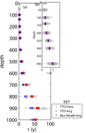
3.2 Mean age of water: τ

Profiles ofτ, the mean age of the water, are shown in Fig. 3. The profile follows an expected pattern of increasing age with depth. The spread in the ages exceeds an-alytical uncertainty. This variability is likely a reflection of heaving of isopycnals: the variation ofτ on an isopycnal surface is relatively small (Fig. 5b) but vertical heave of

5

isopycnal surfaces introduces additional variability when using a depth coordinate sys-tem. The variability does not show any consistent seasonal pattern at depths greater than 140 m. The trend in mean values appears as a smooth function of depth because the variability averages out over many realizations.

The τ determined by the TTD approach is very similar to τ from the box model

10

approach at depths less than or equal to 400 m (blue symbols in Fig. 3). As the depth increases, the two approaches diverge more. The box model approach has an implicit exponential shape to the water mass probability distribution and thus is always skewed towards young ages. In contrast, the TTD model, with_Γ/_{∆ =}1, is mixing waters with a larger age spread and has a non-zero centroid.

15

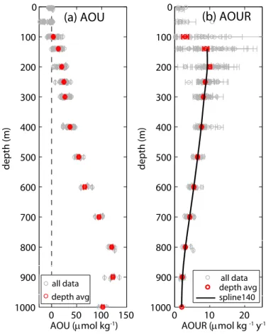
3.3 AOU and AOUR

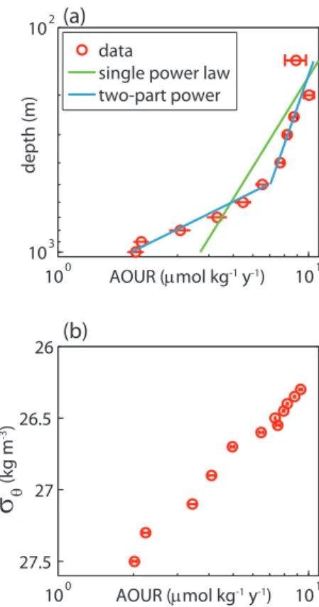
Profiles of AOU and AOUR are shown in Fig. 4. AOU increases with depth since the total amount of organic matter that has been remineralized increases with depth. In contrast, AOUR is largest just below the euphotic zone and then decreases with depth. The depth distribution of AOUR is shown more clearly on a log-log plot (Fig. 5a).

20

The data are not well described by a single power law (i.e. “Martin curve” (Martin et al., 1987)) (reduced chi-squared ₌ 52 for data from 140 m to 1000 m; reduced chi-squared = 31 for data from 200 m to 1000) but rather are better described by two power laws with a break at 500 m (reduced chi-squared ₌ 6 for data from 140 m to 1000 m; reduced chi-squared ₌ 2 for data from 200 m to 1000 m). The exponent of

25

(12)

BGD

8, 9977–10015, 2011

Title Page

Tables Figures

◭ ◮

Back Close

Full Screen / Esc

Discussion

P

a

per

|

Dis

cussion

P

a

per

|

Discussion

P

a

per

|

Discussio

n

P

a

per

|

this break corresponds to waters stemming from different origins – the water shallower than approximately 500 m is primarily mode water which has been directly ventilated from the subtropical North Atlantic recirculation region whereas the deeper water is indirectly ventilated water with a a subpolar and Southern Ocean component (Robbins et al., 2000; Talley, 2003) (see Discussion Sect. 4.1 for more details). The T/3He

5

based method for AOUR is most robust if the water comes from the subtropical North Atlantic since that is the basis for the tritium source function. The Southern Ocean has a very di_fferent tritium source function, making the calculations performed here not quantitative for those deeper waters. Ventilation in the subpolar gyre is less of an issue since the source function di_ffers by only _∼20 %. However, indirect ventilation of the

10

subpolar water may increase the influence of mixing. Therefore, we will concentrate our future discussion on the upper 500 m of data.

We can vertically integrate the AOUR curve in the upper 500 m to achieve a minimum estimate of export flux (minimum because it is only reflective of organic matter reminer-alized in the upper 500 m) of 3.1_±0.1 mol O₂m−2_yr−1_{. Using the revised Redfield ratio}

15

of 1.45 (Anderson and Sarmiento, 1994), this is equivalent to 2.1_±0.08 mol C m−2_yr−1_. The error uncertainty represents the 1σ uncertainty of the standard error of the mean of AOUR at each depth propagated through the integration. It thus takes into account random variations on monthly timescales and thus is likely to include both analytical uncertainty and environmental variability. However, it does not include the systematic

20

uncertainties in the method such as where the water is really coming from, uncertain-ties in the source function, or in the surface solubility value of oxygen. Hence, it is likely an underestimate of the true uncertainty in the AOUR-derived, export flux. When a sensitvity study is performed that takes into account uncertainties in the source func-tion, choice of_Γ/_∆, and surface solubility value of oxygen, the uncertainty in the export

25

flux estimated increases to 0.5 mol O₂m−2_yr−1 _{(see Sect. 4.4). If the box model}

(13)

BGD

8, 9977–10015, 2011

Title Page

Tables Figures

◭ ◮

Back Close

Full Screen / Esc

Discussion

P

a

per

|

Dis

cussion

P

a

per

|

Discussion

P

a

per

|

Discussio

n

P

a

per

|

When the data is binned and plotted as a function of density (Fig. 5b), the error bars are much smaller, suggesting much of the variability seen in the plot vs. depth stems from vertical displacement of isopycnals. Because AOUR of a water parcel averages over multiple trajectories along isopycnal surfaces, as well as over the time since the water has been subducted, it is logical that there will be smaller variability

5

when the data is binned on isopycnal surfaces than when it is binned on constant depth horizons. The data in the upper 500 m corresponds to density surfaces ofσ_θ ₌26.3 to 26.6 kg m−3_{. Thus we also spatially integrated AOUR along those density surfaces} within the recirculation region, i.e. 30◦_{N to 45}◦_{N, 60}◦_{W to 75}◦_{W, to obtain an estimate} of regional export flux of 3.2 Tmol O₂yr−1_{, which is equivalent to 2.2 Tmol C yr}−1 _or

10

approximately 30 Tg C yr−1_.

4 Discussion

4.1 Depth and spatial distribution of AOUR

Export flux is often approximated as a power law distribution with depth based on empirical analyses of sediment trap data (Martin et al., 1987). Since AOUR is equal

15

to the vertical derivative of the export flux, one might expect it to follow a power law as well. If so, then it should plot as a straight line on a log-log plot. The best fit single power law of the AOUR data presented here (Fig. 5a) has an exponent of₋0.55, which is equivalent to a “Martin curve” exponent for export of 0.45 (since AOUR is the derivative of export, the Martin exponent ₌AOUR exponent ₊ 1). A positive Martin

20

exponent would necessitate some initial export flux that does not change with depth in order to avoid the unphysical situation of a negative export flux. In contrast, the Martin et al. (1987) open ocean composite exponent is₋0.858. If one plots sediment trap data from the Sargasso Sea, one can see that the Martin et al curve is not a good fit, with a significant range in flux being apparent at each depth (sediment trap data available at

25

(14)

BGD

8, 9977–10015, 2011

Title Page

Tables Figures

◭ ◮

Back Close

Full Screen / Esc

Discussion

P

a

per

|

Dis

cussion

P

a

per

|

Discussion

P

a

per

|

Discussio

n

P

a

per

|

In spite of the discussion above, one can clearly see that the BATS AOUR data are not described well by a single power law (Fig. 5a) and thus comparing the exponent to Martin et al. (1987) is not particularly fruitful. There are several possible explanations. First, recent work has suggested that a power-law may often not be a good approxima-tion of export flux in the mesopelagic (Lam et al., 2011), and many studies have found

5

large geographic and temporal variability of mesopelagic flux attenuation (Lee et al., 2009; Lomas et al., 2010; Lutz et al., 2007). Second, AOUR may not follow the vertical derivative of a Martin et al. curve, i.e. a single power law originally constructed from sediment trap data as a local estimate of particle sinking, even including the concept that traps sample a spatially larger “statistical funnel” (Siegel et al., 2008; Siegel and

10

Deuser, 1997). In contrast, AOUR reflects the average rate of dissolved and particulate organic matter oxidation along the entire trajectory of a fluid parcel since it left the sur-face, and trajectories can span a range of depths and regional productivities. Because of the shape of the subtropical gyre and the location of BATS near the deepest part of the subtropical bowl, AOUR measured at a given depth includes the influence of higher

15

oxygen consumption rates when water parcels were, at one time, at a much shallower depth.

One can estimate the approximate e_ffect of this bias by comparing the AOUR along an isopycnal path to the local OUR at a fixed depth and location using reasonable es-timates of parcel trajectories. The path-dependent AOUR is simply the OUR averaged

20

in time from the isopycnal outcrop to the sampling location:

AOUR(z_obs,τ)₌1 τ

Zτ

0

OUR(z,t)d t (9)

where z_obs refers to the depth where the AOUR measurement was taken, and z is the time-varying depth trajectory. If one approximates OUR as the derivative of the Martin et al. curve and assumes that the isopycnal trajectory decreases linearly with

25

(15)

BGD

8, 9977–10015, 2011

Title Page

Tables Figures

◭ ◮

Back Close

Full Screen / Esc

Discussion

P

a

per

|

Dis

cussion

P

a

per

|

Discussion

P

a

per

|

Discussio

n

P

a

per

|

approximately a factor of 1.25–1.5 larger than the local OUR at the sampling depth z_obs. A more thorough mathematical treatment of the di_fferences between AOUR and AOU is the subject for a future paper.

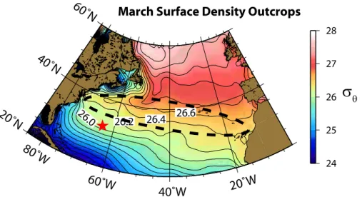
There is a distinct break in the AOUR data at ∼500 m (Fig. 5a), which likely stems from water shallower than 500 m being primarily 18 degree mode water that has formed

5

within the subtropical gyre whereas deeper water has a subpolar and southern ocean component (Robbins et al., 2000; Talley, 2003). The water at BATS shallower than 500 m corresponds to density surfaces of 26.3 to 26.6 kg m−3_{. The March density} out-crops, as calculated from World Ocean Atlas Data (Locarnini et al., 2009; Antonov et al., 2009), are shown in Fig. 6. One can clearly see that the density surfaces of 26.3

10

to 26.6 kg m−3 _{cover a broad area to the north of BATS. Thus, even though we can} re-port an exre-port flux calculated from integrated AOUR at BATS, the flux is representing a much larger geographical area than just BATS. Nonetheless, given the outcrop region, a tritium source function derived for the subtropical North Atlantic is suitable. In con-trast, the water deeper than 500 m, i.e. on density surfaces greater than 26.6 kg m−3_,

15

outcrops further to the north (Fig. 6) as well as sources from the southern ocean. A second way of determining where the water is coming from is to look at maps of the origin of water derived using the transport matrix method (Khatiwala, 2007). Such maps confirm that the water above 500 m at BATS is sourced primarily from the local recirculation region whereas the water below 500 m, however, stems from further afield.

20

In particular, a significant component of the water at depths >800 m stems from the southern ocean. Since the tritium input to the Southern ocean is so di_fferent than that to the North Atlantic, this Southern ocean component makes quantitative interpretation of the deep data di_fficult.

Since AOUR integrates over the entire trajectory of a water parcel along an

isopyc-25

(16)

BGD

8, 9977–10015, 2011

Title Page

Tables Figures

◭ ◮

Back Close

Full Screen / Esc

Discussion

P

a

per

|

Dis

cussion

P

a

per

|

Discussion

P

a

per

|

Discussio

n

P

a

per

|

(related to the age of the water, which ranges from 2 to 5 years in the upper 500 m and much longer below that) is similar to or longer than the time period of our study (3 years). Or it may be because of internal feedbacks that result in ventilation being tied to respiration rates. The water mass formation processes that serve to ventilate/subduct water also tend to bring subsurface nutrients to the euphotic zone by mixing. As

venti-5

lation times increase, fewer nutrients may be replenished in the mixed layer, leading to decreased primary production and possibly decreased remineralization rates. Hence τwould increase but AOU would decrease and thus the AOUR would remain similar.

4.2 Comparison to other estimates of export at BATS

There is a longstanding disagreement over the magnitude of biological production at

10

the BATS site (Michaels et al., 1994). Geochemical tracer based estimates of export production, net community production, and new production suggest biological produc-tion is several times to an order of magnitude higher than estimates based on sediment traps or bottle incubations. This disagreement occurs not only at BATS but also at the Hawaii Ocean Time-series (HOT) and other locations (Burd et al., 2010) and has often

15

been attributed to geochemical estimates averaging over longer spatial and temporal scales than sediment traps or bottle incubations and thus geochemical estimates be-ing more likely to catch episodic high-flux events. AOUR indeed averages over a long spatial and temporal scale – larger scales even than some of the other geochemical techniques such as upper ocean net oxygen and argon balances (Craig and Hayward,

20

1987; Emerson, 1987; Spitzer and Jenkins, 1989) or DIC balances (Keeling et al., 2004; Quay and Stutsman, 2003) for net community production.

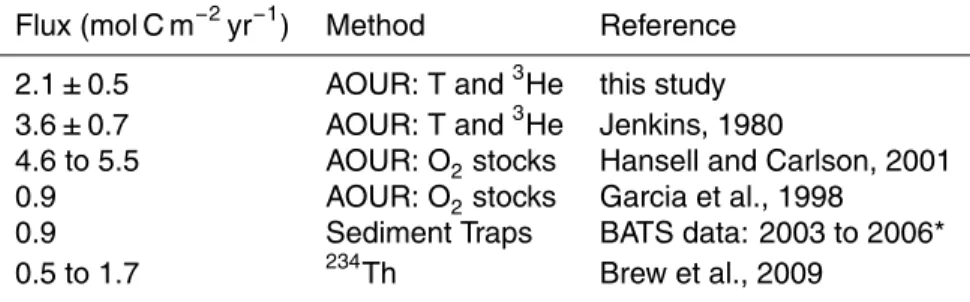
When comparing the estimate of export flux from depth-integrated AOUR reported in this study to other estimates of export flux at BATS (Table 1), one must remember several confounding issues: (1) We calculate export flux by vertically integrating AOUR

25

(17)

BGD

8, 9977–10015, 2011

Title Page

Tables Figures

◭ ◮

Back Close

Full Screen / Esc

Discussion

P

a

per

|

Dis

cussion

P

a

per

|

Discussion

P

a

per

|

Discussio

n

P

a

per

|

et al., 2007). (2) The AOUR method includes the effect of export in dissolved form, i.e. remineralization of DOC, whereas some of the other export techniques (sediment traps and234Th for example) do not. In the subtropical North Atlantic, DOC has been estimated to account 5 % to 28 % of the export flux (Hansell et al., 2004). (3) As de-scribed above, the AOUR estimate is integrating over a large regional area and thus is

5

reflective of a broader region than just the BATS site.

The export flux calculated by vertically integrating the AOUR in the upper 500 m, as reported in this study, is about double the flux calculated from averaging the 150 m sediment trap data from the BATS program (data available at http://bats.bios.edu) over the same 3 year period that the T and 3He data were collected. This difference is

10

too large to likely be accounted for by DOC remineralization and is consistent with the finding that geochemical techniques usually give larger export fluxes than local ones.

Export flux has been measured at BATS through the use of234Th (e.g. (Buesseler et al., 1994). A recent study by Brew et al. (2009), that overlapped in time partially with the AOUR study reported here, quantified carbon export using 234Th to range from

15

1.3_±0.19 to 3.91_±0.52 mmol C m−2_d−1_{. If one scales these numbers up to annual}

numbers, they suggest a range of 0.48 to 1.7 mol C m−2_yr−1_{. The upper end of this} range is approaching our AOUR-derived flux. Since the AOUR-derived flux averages over much longer spatial and temporal scales than234Th (a few years rather than a month), it is reasonable to expect that the AOUR-derived flux would capture more of

20

rare high flux events and thus would be at the upper end of the range or larger than the

234_{Th flux.}

The export flux reported here is somewhat smaller than export calculated from AOUR based on tritium-helium data by previous studies. In large part, this is due to our study reporting a lower bound of export (500 m only) whereas the other studies

25

(18)

BGD

8, 9977–10015, 2011

Title Page

Tables Figures

◭ ◮

Back Close

Full Screen / Esc

Discussion

P

a

per

|

Dis

cussion

P

a

per

|

Discussion

P

a

per

|

Discussio

n

P

a

per

|

the export flux determined in this study (see Sect. 4.3 for an in-depth comparison of changing AOUR through time). The export flux we report is in the middle of two other estimates of export flux based on AOUR, which were both calculated using standing stocks of oxygen (Garcia et al., 1998; Hansell and Carlson, 2001).

4.3 Apparent AOUR changes through time

5

The oxygen content of the ocean has been reported to be decreasing (Stramma et al., 2008, 2010; Whitney et al., 2007). Is this decrease due to physical mechanisms, i.e. changes in ventilation, or to biogeochemical ones, i.e. changes in export flux? AOUR is a tool that can help us answer this question since it allows calculation of the water age (τ) as well as the biological oxygen demand (AOU). Thus we did a detailed

10

comparison between AOUR reported in this paper and AOUR from 20 to 30 years ago. For the older time period, we used tritium and helium data collected in the 1970s and 1980s at the Station S site (32◦₁₀′_{N, 64}◦₃₀′_{W), which is 15 nautical miles from the} BATS site (Jenkins, 1980, 1988, 1998). When Jenkins published the data, he used a box model approach to calculateτ. Here, we applied the same TTD approach that we

15

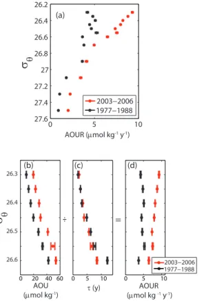
used for the 2003 to 2006 data (described in Sect. 2.2) to ensure that any di_fferences inτ were not the result of calculation methods. We found that AOUR in 2003 to 2006 was significantly greater than AOUR in the 1970s and 1980s (Fig. 7a). This di_fference was most pronounced in the upper 500 m (σ_θ<26.6 kg m−3_{), the area where we have} the most confidence in our approach.

20

What is the cause for this increase in AOUR with time? When we look at the AOUR in terms of its two components – AOU andτ(Fig. 7b and c), we see thatτis the same, within errors, in the two time periods but that AOU was significantly lower in 1977– 1877 than in 2003–2006. Thus the change in AOUR is not due to physical changes in ventilation but rather due to the biogeochemical changes associated with a changing

25

(19)

BGD

8, 9977–10015, 2011

Title Page

Tables Figures

◭ ◮

Back Close

Full Screen / Esc

Discussion

P

a

per

|

Dis

cussion

P

a

per

|

Discussion

P

a

per

|

Discussio

n

P

a

per

|

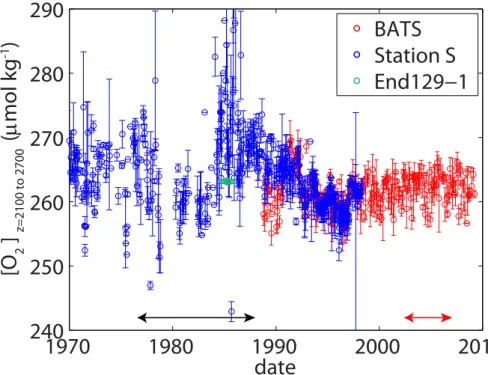
Examination of the deep oxygen record (2100 to 2700 m) from Station S and BATS over the last thirty years supports the conclusion that the di_fference in AOU is likely due to methodological artefacts (Fig. 8). Oxygen in these deep waters should not change much with time given the long residence time of oxygen below the range of most organic matter remineralization. However, when one looks at the oxygen record,

5

one can see that the deep O₂data from Station S in the 1970s and 1980s is much more scattered and significantly greater than the deep BATS data or Station S data from 1992 onwards. In particular, the time period between 1985 and 1987 has particularly large deep O₂ concentrations, which are on average 9.8 µmol kg−1 _{larger than during} 2003–2006. Furthermore, O₂concentrations from a location near Station S (32.332◦N,

10

64 ˙200◦_{W) performed by a di}

fferent lab as part of station 50 on the R/VEndeavor 129– 1 cruise, yield deep O₂concentrations in 1985 of 263.2_±0.2 µmol kg−1_{(Knapp, 1988),} which is very similar to the 2003 to 2006 BATS deep O₂concentrations (262.2_±2) but significantly lower than the 1985 Station SO₂data (274±12).

The fact that the apparent di_fferences in AOUR between 2003 and 2006 and the

15

1980s as reported here is likely due to methodological artefacts suggests that caution should be used when O₂inventories are compared at other locations as well. Old O₂ data from other locations may have methodological artefacts as well and should be examined carefully before conclusions on ocean deoxygenation are made.

4.4 Uncertainties and sensitivity studies

20

There are a number of sources of uncertainty in the AOUR estimates and export flux reported in this paper. Here we perform a sensitivity study of the depth-integrated AOUR to some of the parameters used in the calculations. We then discuss some other sources of errors that are not easily quantifiable.

For water shallower than 500 m, the source of the water is likely the subtropical North

25

(20)

BGD

8, 9977–10015, 2011

Title Page

Tables Figures

◭ ◮

Back Close

Full Screen / Esc

Discussion

P

a

per

|

Dis

cussion

P

a

per

|

Discussion

P

a

per

|

Discussio

n

P

a

per

|

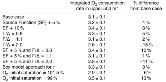
changes in the source function. There is approximately a 10 % increase in tritium for every 10 degrees north of Bermuda (Doney and Jenkins, 1988). If the source func-tion is 10 % larger, than the export flux increases to 3.3_±0.1 mol O₂m−2_yr−1_{, a 8 %} increase (Table 2). This suggests that the error added by source function, in water shallower than 500 m, is less than 10 %. For waters deeper than 500 m, the problem is

5

more severe. Some fraction of the deeper water is sourced from the Southern Ocean where there is likely a very di_fferent tritium source function, given that the tritium load-ing was primarily in the Northern Hemisphere (Doney et al., 1992). We thus do not perform a quantitative interpretation of our deeper data in this paper; that will be the topic of a future paper.

10

A second issue to consider when calculatingτis that the results are sensitive to the choice of_Γ and _∆. Since we have two transient tracers – both T and3He – we use the data shallower than 500 m (density less than 26.6 kg m−3_{) and the TTD equations}

in order to constrain the ratio of_Γ/_∆ (Fig. 9). Specifically, we use a range of _Γ from 0 to 200, apply di_fferent _Γ/_∆ ratios (e.g. 0.8, 0.9, 1, 1.1, 2) to calculate _∆, and then

15

calculateG according to Eq. 3. We next use the source function (Eq. 2), which has been decay corrected, andG in order to calculate 3He and T values. We plot those

3

He and T values (colored curves in Fig. 9) alongside the T and3He data measured (black squares) in order to determine a range of_Γ/_∆that gives a reasonable fit to the data. Using the data from this study, Γ/∆ could range between 0.8 and 2.0. If Γ/∆

20

is 0.8, then the export flux increases by 5 % to 3.3_±0.1 mol O₂m−2_yr−1 _{(Table 2). If}

Γ/_{∆ =}2.0, then the export flux decreases by 15 % to 2.64_±0.1 mol O₂m−2_yr−1_{. Using} data from previous studies (Jenkins, 1980, 1988, 1998) allows a better constraint since T and 3He were higher in the upper thermocline during the 1970s and 1980s. The older data further constrains_Γ/_∆to be between 0.8 and 1.1. If_Γ/_{∆ =} 1.1, the export

25

flux decreases by 3 % to 3.05_±0.1 mol O₂m−2_yr−1_{. Thus a reasonable range of}

(21)

BGD

8, 9977–10015, 2011

Title Page

Tables Figures

◭ ◮

Back Close

Full Screen / Esc

Discussion

P

a

per

|

Dis

cussion

P

a

per

|

Discussion

P

a

per

|

Discussio

n

P

a

per

|

If instead of using the TTD approach we use the box model approach (Jenkins, 1980), which is shown in Fig. 9 to do a good job at fitting the T and3He data, then the depth-integrated AOUR increases by 6 % to 3.3_±0.1 mol O₂m−2_yr−1_.

An added source of uncertainty stems from the assumption implicit in AOU that the oxygen at the surface was in equilibrium. However, in the surface ocean, oxygen is

5

often not at equilibrium. O₂measurements at BATS can give us an idea of the expected the deviation of O₂from equilibrium. Measurements of O₂in the mixed layer at BATS show that O₂ ranges from being undersaturated by approximately 1 % to 2 % in the winter to being supersaturated by 2 % to 3 % in the summer (http://www.bios.bats.edu/). Stommel (1979) argued that a “demon” selectively pumps late winter water into the

10

main thermocline. Modeling experiments confirmed Stommel’s hypothesis finding that the subduction period lasts about one month after the end of winter (Williams et al., 1995). In the late winter/early spring at BATS, the O₂ saturation ranges from 99 % to 101.5 % depending upon the year (http://www.bios.bats.edu/). If we calculate the depth-integrated AOUR assuming surface water is at 99 % of saturation value, then

15

we determine the depth-integrated AOUR from 140 to 500 m to be 2.9 mol O₂m−2_yr−1_,

a decrease of 6 % over our initial calculation. If we use 101.5 % of saturation value, the value is 3.5 mol O₂m−2_yr−1_{, an increase of 12 %. Thus uncertainty in the initial} saturation value of O₂leads to an uncertainty of approximately 12 % in our calculations. If we add in quadrature conservative estimates of the uncertainty from the source

20

function (8 %), choice of_Γ/_∆(8 %, note: we do not include the_Γ/_{∆ =}2 choice since it is shown to be too pessimistic by earlier data), initial oxygen saturation (13 %), and mea-surement uncertainty (3 %), then the total uncertainty on the depth-integrated AOUR number is 0.5 mol O₂m−2_yr−1_{, a 16 % uncertainty.}

A limitation in the calculation of the export flux presented here is that we are only

25

(22)

BGD

8, 9977–10015, 2011

Title Page

Tables Figures

◭ ◮

Back Close

Full Screen / Esc

Discussion

P

a

per

|

Dis

cussion

P

a

per

|

Discussion

P

a

per

|

Discussio

n

P

a

per

|

at 140 m is a minimum estimate. Indeed, one can see the effect of this mixing when one looks at the seasonal cycle of AOUR at 140 m, where there is a dramatic decline in AOUR each January.

We did not calculate export production above 140 m using this approach and yet we know that oxygen consumption is occurring at shallower depths. Export is often

5

defined as organic matter remineralized below the euphotic zone, which would be ap-proximately 100 m at BATS. A recent study used7Be to estimate oxygen consumption rates in the upper 200 m of the ocean at BATS and found a depth-integrated oxygen consumption rate of 4.5_±0.4 mol O₂m−2_yr−1_{between 100 and 200 m (Kadko, 2009) –} this is comparable to our entire estimate of oxygen consumption from 140 m to 500 m.

10

It is not possible from the Kadko study to know what proportion of the estimated oxygen consumption occurred between 100 and 140 m (missed in our study) and which was between 140 and 200 m (included in our study). Nonetheless, the point remains that there is significant export in the upper 200 m that we may not be properly accounting for.

15

5 Conclusions

We have presented AOUR for a three year time period at the BATS site as determined by tritium and 3He data. We find that the depth integrated oxygen consumption be-tween 140 m and 500 m is 3.1 mol_±0.5 mol O₂m−2_yr−1_{. This estimate is a minimum}

estimate of export at BATS since substantial oxygen consumption may be occurring

20

above 140 m and below 500 m. This estimate of export is reflective of large spatial and temporal scales – the spatial scale is approximately that of the recirculation region and the temporal scale is that of several years. We sampled at monthly resolution and find very little variation of AOUR when the data is binned on isopycnal surfaces, likely a re-flection of the long spatial and temporal scales of the measurement but also suggestive

25

(23)

BGD

8, 9977–10015, 2011

Title Page

Tables Figures

◭ ◮

Back Close

Full Screen / Esc

Discussion

P

a

per

|

Dis

cussion

P

a

per

|

Discussion

P

a

per

|

Discussio

n

P

a

per

|

We compared AOUR presented in this study to AOUR calculated based on earlier tritium and3He data and found a large increase in AOUR over the past thirty years. This increase is due to an increase in AOU and is more likely associated with methodological artefacts in the oxygen data from the 1980s rather than due to any climatic-associated change in production or remineralization.

5

Acknowledgements. We are grateful to Mike Lomas, Rod Johnson, the BATS technicians and the captain and crew of the R/VWeatherbird IIand R/V Atlantic Explorerfor their support in col-lecting data for this study. Support from this work came from the National Science Foundation (OCE-0221247and OCE-0623034) and from the WHOI Penzance Endowed Fund in Support of Assistant Scientists.

10

References

Anderson, L. A. and Sarmiento, J. L.: Redfield ratios of remineralization determined by nutrient data-analysis, Global Biogeochem. Cy., 8, 65–80, 1994.

Antonov, J. I., Seidov, D., Boyer, T. P., Locarnini, R. A., Mishonov, A. V., Garcia, H. E., Baranova, O. K., Zweng, M. M., and Johnson, D. R.: World Ocean Atlas 2009, Volume 2: Salinity, edited

15

by: Levitus, S., US Government Printing Office, Washington D.C., 184 pp., 2009.

Benson, B. B. and Krause, D., Jr.: Isotopic fractionation of helium during solution: a probe for the liquid state, J. Solution Chem., 9, 895–909, 1980.

Bopp, L., Le Quere, C., Heimann, M., Manning, A. C., and Monfray, P.: Climate-induced oceanic oxygen fluxes: Implications for the contemporary carbon budget, Global Biogeochem. Cy.,

20

16, 1022, doi:10.1029/2001gb001445, 2002.

Brew, H. S., Moran, S. B., Lomas, M. W., and Burd, A. B.: Plankton community composition, or-ganic carbon and thorium-234 particle size distributions, and particle export in the Sargasso Sea, J. Mar. Res., 67, 845–868, 2009.

Buesseler, K. O., Michaels, A. F., Siegel, D. A., and Knap, A. H.: A three dimensional

time-25

dependent approach to calibrating sediment trap fluxes, Global Biogeochem. Cy., 12, 297– 310, 1994.

(24)

BGD

8, 9977–10015, 2011

Title Page

Tables Figures

◭ ◮

Back Close

Full Screen / Esc

Discussion

P

a

per

|

Dis

cussion

P

a

per

|

Discussion

P

a

per

|

Discussio

n

P

a

per

|

M. W., Steinberg, D. K., Valdes, J., Van Mooy, B., and Wilson, S.: Revisiting carbon flux through the ocean’s twilight zone, Science, 316, 567–570, 2007.

Buesseler, K. O., Lamborg, C., Cai, P., Escoube, R., Johnson, R., Pike, S., Masque, P., McGillicuddy, D., and Verdeny, E.: Particle fluxes associated with mesoscale eddies in the Sargasso Sea, Deep-Sea Res. Pt. II, 55, 1426–1444, doi:10.1016/j.dsr2.2008.02.007, 2008.

5

Burd, A. B., Hansell, D. A., Steinberg, D. K., Anderson, T. R., Aristegui, J., Baltar, F., Beaupre, S. R., Buesseler, K. O., DeHairs, F., Jackson, G. A., Kadko, D. C., Koppelmann, R., Lampitt, R. S., Nagata, T., Reinthaler, T., Robinson, C., Robison, B. H., Tamburini, C., and Tanaka, T.: Assessing the apparent imbalance between geochemical and biochemical indicators of meso- and bathypelagic biological activity: What the @$#! is wrong with present calculations

10

of carbon budgets?, Deep-Sea Res. Pt. II, 57, 1557–1571, doi:10.1016/j.dsr2.2010.02.022, 2010.

Codispoti, L. A., Brandes, J. A., Christensen, J. P., Devol, A. H., Naqvi, S. W. A., Paerl, H. W., and Yoshinari, T.: The oceanic fixed nitrogen and nitrous oxide budgets: Moving targets as we enter the anthropocene?, Sci. Mar., 65, 85–105, 2001.

15

Craig, H. and Hayward, T.: Oxygen supersaturation in the ocean: biological versus physical contributions, Science, 235, 199–202, 1987.

Deutsch, C., Brix, H., Ito, T., Frenzel, H., and Thompson, L.: Climate-Forced Variability of Ocean Hypoxia, Science, 333, 336-339, 10.1126/science.1202422, 2011.

Doney, S. C. and Jenkins, W. J.: The effect of boundary conditions on tracer estimates of

20

thermocline ventilation rates, J. Mar. Res., 46, 947–965, 1988.

Doney, S. C. and Bullister, J. L.: A chlorofluorocarbon section in the eastern North Atlantic, Deep-Sea Res., 39, 1857–1883, doi:10.1016/0198-0149(92)90003-c, 1992.

Doney, S. C., Glover, D. M., and Jenkins, W. J.: A Model Function of the Global Bomb Tri-tium Distribution in Precipitation 1960-1986, J. Geophys. Res.-Oceans, 97, 5481–5492,

25

doi:10.1029/92jc00015, 1992.

Dreisigacker, E. and Roether, W.: Tritium and90Sr in North Atlantic surface water, Earth Planet. Sc. Lett., 38, 301–312, 1978.

Emerson, S.: Seasonal Oxygen Cycles and Biological New Production in Surface Waters of the Sub-Arctic Pacific-Ocean, J. Geophys. Res.-Oceans, 92, 6535–6544, 1987.

30

(25)

BGD

8, 9977–10015, 2011

Title Page

Tables Figures

◭ ◮

Back Close

Full Screen / Esc

Discussion

P

a

per

|

Dis

cussion

P

a

per

|

Discussion

P

a

per

|

Discussio

n

P

a

per

|

Garcia, H. E. and Gordon, L. I.: Oxygen solubility in water: better fitting equations, Limnol. Oceanogr., 37, 1307–1312, 1992.

Hall, T. M., Waugh, D. W., Haine, T. W. N., Robbins, P. E., and Khatiwala, S.: Estimates of anthropogenic carbon in the Indian Ocean with allowance for mixing and time-varying air-sea CO2 disequilibrium, Global Biogeochem. Cy., 18, Gb1031, doi:10.1029/2003gb002120,

5

2004.

Hansell, D. A. and Carlson, C. A.: Biogeochemistry of total organic carbon and nitrogen in the Sargasso Sea: control by convective overturn, Deep-Sea Res. Pt. II, 48, 1649–1667, 2001. Hansell, D. A., Bates, N. R., and Olson, D. B.: Excess nitrate and nitrogen fixation in the North

Atlantic Ocean, Mar. Chem., 84, 243–265, 2004.

10

Jenkins, W. J.: Tritium-Helium dating in Sargasso Sea – measurement of oxygen utilization rates, Science, 196, 291–292, 1977.

Jenkins, W. J.: Tritium and He-3 in the Sargasso Sea, J. Mar. Res., 38, 533–569, 1980. Jenkins, W. J.: The use of anthropogenic tritium and He-3 to study sub-tropical gyre ventilation

and circulation, Philos. Trans. R. Soc. Lond. Ser. A-Math. Phys. Eng. Sci., 325, 43–61, 1988.

15

Jenkins, W. J.: Studying subtropical thermocline ventilation and circulation using tritium and He-3, J. Geophys. Res.-Oceans, 103, 15817–15831, 1998.

Kadko, D.: Rapid oxygen utilization in the ocean twilight zone assessed with the cos-mogenic isotope (7)Be (vol 23, GB4010, 2009), Global Biogeochem. Cy., 23, Gb4099, doi:10.1029/2009gb003706, 2009.

20

Keeling, C. D., Brix, H., and Gruber, N.: Seasonal and long-term dynamics of the upper ocean carbon cycle at Station ALOHA near Hawaii, Global Biogeochem. Cy., 18, GB4006, doi:10.1029/2004GB002227, 2004.

Keeling, R. F., Kortzinger, A., and Gruber, N.: Ocean Deoxygenation in a Warming World, Annu. Rev. Mar. Sci., 2, 199–229, doi:10.1146/annurev.marine.010908.163855, 2010.

25

Khatiwala, S.: A computational framework for simulation of biogeochemical tracers in the ocean, Global Biogeochem. Cy., 21, Gb3001, doi:10.1029/2007gb002923, 2007.

Khatiwala, S., Primeau, F., and Hall, T.: Reconstruction of the history of anthropogenic CO(2) concentrations in the ocean, Nature, 462, 346–350, doi:10.1038/nature08526, 2009. Knap, A. J., Michaels, A. F., Steinberg, D. K., and et al.: BATS methods manual, Version 4, US

30

JGOFS Planning Office, Woods Hole, MA, 1997.

(26)

BGD

8, 9977–10015, 2011

Title Page

Tables Figures

◭ ◮

Back Close

Full Screen / Esc

Discussion

P

a

per

|

Dis

cussion

P

a

per

|

Discussion

P

a

per

|

Discussio

n

P

a

per

|

Lam, P. J., Doney, S. C., and Bishop, J. K. B.: The dyanmic ocean biological pump: Insights from a global compilation of particulate organic carbon, CaCO3, and opal concentration profiles

from the mesopelagic, Global Biogeochem. Cy., 25, GB3009, doi:10.1029/2010GB003868, 2011.

Lee, C., Peterson, M. L., Wakeham, S. G., Armstrong, R. A., Cochran, J. K., Miquel, J. C.,

5

Fowler, S. W., Hirschberg, D., Beck, A., and Xue, J. H.: Particulate organic matter and ballast fluxes measured using time-series and settling velocity sediment traps in the northwestern Mediterranean Sea, Deep-Sea Res. Pt. II, 56, 1420–1436, doi:10.1016/j.dsr2.2008.11.029, 2009.

Locarnini, R. A., Mishonov, A. V., Antonov, J. I., Boyer, T. P., Garcia, H. E., Baranova, O. K.,

10

Zweng, M. M., and Johnson, D. R.: World Ocean Atlas 2009, Volume 1: Temperature, edited by: Levitus, S., U.S. Government Printing Office, Washington D.C., 184 pp., 2009.

Lomas, M. W., Steinberg, D. K., Dickey, T., Carlson, C. A., Nelson, N. B., Condon, R. H., and Bates, N. R.: Increased ocean carbon export in the Sargasso Sea linked to climate variability is countered by its enhanced mesopelagic attenuation, Biogeosciences, 7, 57–70,

15

doi:10.5194/bg-7-57-2010, 2010.

Lott, D. E. and Jenkins, W. J.: Advances in analysis and shipboard processing of tritium and helium samples, International WOCE Newsletter, 30, 27–30, 1998.

Lutz, M. J., Caldeira, K., Dunbar, R. B., and Behrenfeld, M. J.: Seasonal rhythms of net primary production and particulate organic carbon flux to depth describe the effi

-20

ciency of biological pump in the global ocean, J. Geophys. Res.-Oceans, 112, C10011, doi:10.1029/2006jc003706, 2007.

MacMahon, D.: Half-life evaluations for H-3, Sr-90, and Y-90, Appl. Radiat. Isotopes, 64, 1417– 1419, 2006.

Maiti, K., Benitez-Nelson, C. R., and Buesseler, K. O.: Insights into particle formation and

25

remineralization using the short-lived radionuclide, Thoruim-234, Geophys. Res. Lett., 37, L15608, doi:10.1029/2010gl044063, 2010.

Martin, J. H., Knauer, G. A., Karl, D. M., and Broenkow, W. W.: VERTEX: carbon cycling in the northeast Pacific, Deep-Sea Res., 34, 267–285, 1987.

Matear, R. J. and Hirst, A. C.: Long-term changes in dissolved oxygen concentrations

30

in the ocean caused by protracted global warming, Global Biogeochem. Cy., 17, 1125, doi:10.1029/2002gb001997, 2003.

(27)

BGD

8, 9977–10015, 2011

Title Page

Tables Figures

◭ ◮

Back Close

Full Screen / Esc

Discussion

P

a

per

|

Dis

cussion

P

a

per

|

Discussion

P

a

per

|

Discussio

n

P

a

per

|

Study and the Hydrostation S program, Deep-Sea Res. Pt. II, 43, 157–198, 1996.

Michaels, A. F., Bates, N. R., Buesseler, K. O., Carlson, C. A., and Knap, A. H.: Carbon system imbalances in the Sargasso Sea, Nature, 372, 537–540, 1994.

Plattner, G. K., Joos, F., Stocker, T. F., and Marchal, O.: Feedback mechanisms and sensitivities of ocean carbon uptake under global warming, Tellus B, 53, 564–592,

doi:10.1034/j.1600-5

0889.2001.530504.x, 2001.

Quay, P. and Stutsman, J.: Surface layer carbon budget for the subtropical N. Pacific: delta C-13 constraints at station ALOHA, Deep-Sea Res. Pt. I, 50, 1045–1061, 2003.

Robbins, P. E., Price, J. F., Owens, W. B., and Jenkins, W. J.: The importance of lateral dif-fusion for the ventilation of the lower thermocline in the subtropical North Atlantic, J. Phys.

10

Oceanogr., 30, 67–89, 2000.

Siegel, D. A. and Deuser, W. G.: Trajectories of sinking particles in the Sargasso Sea: modeling of statistical funnels above deep-ocean sediment traps, Deep-Sea Res. Pt. I, 44, 1519–1541, doi:10.1016/s0967-0637(97)00028-9, 1997.

Siegel, D. A., Fields, E., and Buesseler, K. O.: A bottom-up view of the biological pump:

15

Modeling source funnels above ocean sediment traps, Deep-Sea Res. Pt. I, 55, 108–127, doi:10.1016/j.dsr.2007.10.006, 2008.

Smethie, W. M. and Fine, R. A.: Rates of North Atlantic Deep Water formation calculated from chlorofluorocarbon inventories, Deep-Sea Res. Pt. I, 48, 189–215, doi:10.1016/s0967-0637(00)00048-0, 2001.

20

Spitzer, W. S. and Jenkins, W. J.: Rates of vertical mixing, gas-exchange and new production - estimates from seasonal gas cycles in the upper ocean near Bermuda, J. Mar. Res., 47, 169–196, 1989.

Stanley, R. H. R., Buesseler, K. O., Manganini, S. J., Steinberg, D. K., and Valdes, J. R.: A comparison of major and minor elemental fluxes collected in neutrally buoyant and

surface-25

tethered sediment traps, Deep-Sea Res. Pt. I, 51, 1387–1395, 2004.

Stanley, R. H. R., Baschek, B., Lott, D. E., and Jenkins, W. J.: A new automated method for measuring noble gases and their isotopic ratios in water samples, Geochem. Geophys. Geosy., 10, doi:10.1029/2009GC002429, 2009.

Steinberg, D. K., Carlson, C. A., Bates, N. R., Johnson, R. J., Michaels, A. F., and Knap, A.

30