Patterning and Incorporating MicroRNA Regulation
Jerry S. Chen1,2, Abygail M. Gumbayan2, Robert W. Zeller1,2, Joseph M. Mahaffy1,3*
1Computational Science Research Center, San Diego State University, San Diego, California, United States of America,2Department of Biology, San Diego State University, San Diego, California, United States of America,3Department of Mathematics and Statistics, San Diego State University, San Diego, California, United States of America
Abstract
Notch-Delta signaling is a fundamental cell-cell communication mechanism that governs the differentiation of many cell types. Most existing mathematical models of Notch-Delta signaling are based on a feedback loop between Notch and Delta leading to lateral inhibition of neighboring cells. These models result in a checkerboard spatial pattern whereby adjacent cells express opposing levels of Notch and Delta, leading to alternate cell fates. However, a growing body of biological evidence suggests that Notch-Delta signaling produces other patterns that are not checkerboard, and therefore a new model is needed. Here, we present an expanded Notch-Delta model that builds upon previous models, adding a local Notch activity gradient, which affects long-range patterning, and the activity of a regulatory microRNA. This model is motivated by our experiments in the ascidianCiona intestinalisshowing that the peripheral sensory neurons, whose specification is in part regulated by the coordinate activity of Notch-Delta signaling and the microRNA miR-124, exhibit a sparse spatial pattern whereby consecutive neurons may be spaced over a dozen cells apart. We perform rigorous stability and bifurcation analyses, and demonstrate that our model is able to accurately explain and reproduce the neuronal pattern inCiona. Using Monte Carlo simulations of our model along with miR-124 transgene over-expression assays, we demonstrate that the activity of miR-124 can be incorporated into the Notch decay rate parameter of our model. Finally, we motivate the general applicability of our model to Delta signaling in other animals by providing evidence that microRNAs regulate Notch-Delta signaling in analogous cell types in other organisms, and by discussing evidence in other organisms of sparse spatial patterns in tissues where Notch-Delta signaling is active.
Citation:Chen JS, Gumbayan AM, Zeller RW, Mahaffy JM (2014) An Expanded Notch-Delta Model Exhibiting Long-Range Patterning and Incorporating MicroRNA Regulation. PLoS Comput Biol 10(6): e1003655. doi:10.1371/journal.pcbi.1003655
Editor:Qing Nie, University of California, Irvine, United States of America
ReceivedDecember 12, 2013;AcceptedApril 23, 2014;PublishedJune 19, 2014
Copyright:ß2014 Chen et al. This is an open-access article distributed under the terms of the Creative Commons Attribution License, which permits unrestricted use, distribution, and reproduction in any medium, provided the original author and source are credited.
Funding:Funding provided by NSF Grant IOS-0951347 to RWZ (www.nsf.gov). The funders had no role in study design, data collection and analysis, decision to publish, or preparation of the manuscript.
Competing Interests:The authors have declared that no competing interests exist. * Email: [email protected]
Introduction
Differentiation of tissues during early animal development as well as tissue homeostasis during adulthood requires constant communication between cells. One of the most common ways by which cells communicate with each other is through the Notch-Delta signaling pathway [1–4]. Notch-Notch-Delta signaling is a fundamental cell-to-cell communication mechanism whereby a bound Delta ligand in one cell binds to a membrane-bound Notch receptor in a neighboring cell, generating a particular downstream response that depends on cellular context [1,5]. Studies in several animals have shown that Notch expression is both temporally and spatially widespread [2–4,6,7]. It is not surprising, then, that Notch-Delta signaling is involved in the development and homeostasis of many tissues, most notably those of the nervous system [7], but also within the heart, kidney, liver, pancreas, breast, inner ear, prostate, thyroid, respiratory system, immune system, and many other cell types (reviewed in [1]).
Although the specific molecular factors and interactions are remarkably complex and vary among different organisms and cell types, the core Notch signaling pathway is relatively simple and is conserved across all bilaterian animals [1,3]. The core pathway consists of five main components: a Notch receptor, a CSL family
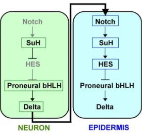
transcription factor (TF), the Hairy and Enhancer-of-split (Hes) family of TFs, the basic helix-loop-helix (bHLH) proneural TFs, and a Delta ligand (Figure 1). In most animals there are multiple genes that encode each component. For example, mammals have four Notch receptor genes and at least seven genes for Hes family members that mediate Notch-Delta signaling in different tissues [8,9].
[15–17]. Finally, the transcription factor CSL functions as a repressor of Hes family members in the signal-sending cell but becomes an activator of Hes genes in the signal-receiving cell [18,19]. This functional switch of CSL from repressor to activator occurs when the intracellular domain (ICD) of Notch translocates to the nucleus where it displaces a co-repressor complexed with CSL [2].
With this biological background in hand, several mathematical and computational models have been developed over the years to try and quantitatively explain the dynamics of Notch-Delta signaling [12,20–24]. These Notch-Delta models usually fall into one of two categories: comprehensive models and minimal models. In comprehensive models, all of the experimentally validated (and sometimes solely computationally predicted) molecular compo-nents are represented as separate variables, and all of the known or predicted interactions are represented as separate equations in the model [23,24]. Although complex, these models have led to some key insights into the specific dynamics of particular Notch-Delta pathway genes. For example, one model that incorporated extensive feedback between Notch, CSL, and Hes resolved the long-standing issue that Hes can act both as a bistable switch and as an oscillator by showing that the transition between these two states can occur by tuning a single parameter, the Hes1 repression constant [23]. Another model incorporating Goodwin-modified biochemical kinetic equations for transcription, nuclear export, translation, and DNA-binding and dimerization of each factor showed the importance of the decay rate of Hes1 [24]. However, one drawback of comprehensive models is that they are usually based on experimental data from one particular cell type and, therefore, are not generalizable to other systems.
By contrast, in minimal models only the core molecular components and interactions, which capture the overall, essential Notch-Delta signaling dynamics, are represented in the differential equations. Unlike comprehensive models, minimal models have the advantage of being applicable to many biological contexts and are also more amenable to parameter sensitivity and stability analyses, which can shed important insight into the dynamics of the system. The first minimal Notch-Delta model was published by Monk and colleagues [20], which at its core is a simple two-cell model with a feedback loop involving just two variables: Notch and Delta. Because the core cascade is essentially linear, they postulated that the Notch variable could represent the quantity of
activated Notch protein (i.e., Notch ICD) in the cell or the quantity of downstream Hes TF [20]. The production functions represent-ing Notch-Delta interactions could be modeled usrepresent-ing Hill functions, which are commonly used to model protein-protein as well as protein-DNA interactions [12,20,25] and for which we now have extensive experimental confirmation through biochemical studies [12,26]. Through their model, Monk and colleagues demonstrated that such a feedback model results in a checker-board spatial expression pattern of Notch and Delta, which mimics the Notch-Delta pattern found in several biological contexts for which lateral inhibition occurs [20,21,27]. With lower coopera-tivity (i.e., a lower Hill coefficient), occasionally a spacing of two or three cells can occur [20]. Subsequent models over the next several years were for the most part variations of the original Monk model (e.g., [21,22]). Eventually, growing experimental evidence of cis-inhibition of Notch by Delta led to an updated model by Elowitz and colleagues that incorporated this interaction [12]. Such cis-inhibition was thought to facilitate Notch-Delta lateral cis-inhibition, and indeed the expanded model resulted in faster dynamics, sharper checkerboard patterning and greater robustness to noise [12].
While the Monk and Elowitz models can explain the patterning in some biological systems such as ciliated cells in the early Xenopus ectoderm [21], there are cases in both invertebrates [28– 34] and vertebrates [7,35–37], where Notch-Delta signaling is clearly active but the pattern is not checkerboard. In many cases, the pattern is much more random and sparse, where the spacing between signal-sending cells can range from a single cell to dozens of cells in between [30,31,33]. For example, studies in zebrafish and chick neuroepithelial tissues have demonstrated a gradient of expression for Notch and/or Delta [7,36,37]. Also, the sensory organ precursor (SOP) cells of theDrosophilathorax that give rise to microchaetes are spaced about five cells apart when fully developed [5,28–30,38]. A pair of studies demonstrated that SOPs in wild-type Drosophila extend dynamic projections called filopodia, and that these filopodia express graded amounts of Delta along the filopoidia and allow the SOPs to reach out and activate Notch signaling in non-neighboring cells [30,31]. Another form of extended communcation in Notch signaling can occur through a process called lateral induction, in which a Delta-bound Notch receptor in the signal-receiving cell can induce the expression of other ligands, which signal Notch in downstream cells [39–41]. Several authors analyzed more generalized models[42–44] with nearest neighbor or juxtacrine inhibition and induction and found these systems could generate Turing solutions[45] from a homogeneous steady-state with various wavelengths. Thus, a model for a juxtacrine system can produce stable periodic patterns with larger spacing between peaks of Delta activity. Hence, in addition to neighboring-cell lateral inhibition, a form of commu-nication leading to long-range patterning can also operate in the context of Notch-Delta signaling. Since these filopodia are wide at the base but gradually thin out towards the tip, this suggests a concentration gradient where cells touching near the base of filopodia receive stronger Notch activation compared to cells in contact with the tips.
In this report, we present a minimal Notch-Delta model, which expands upon the previous Monk and Elowitz models [12,20] by adding a simple nearest-neighbor Notch gradient term that makes it possible for the system to exhibit long-range effects on cell morphogenesis. We show that incorporation of a Notch activity gradient term is able to produce a sparse pattern of Delta expression whereby Delta-expressing cells can be spaced many cells apart. In our studies, we focus on the patterning of larval tail epidermal sensory neurons (ESNs) within the peripheral nervous Author Summary
system (PNS) of the ascidian Ciona intestinalis. We quantify the number and spacing of ESNs in wild-type larvae, and show that our expanded Notch-Delta model accurately reproduces the experimentally observed ESN pattern [33,34,46]. Ascidians are invertebrate chordates and are the closest invertebrate relatives of vertebrates [47]. As such, they occupy an important phylogenetic position for understanding how molecular developmental path-ways evolved when invertebrates and vertebrates diverged from their last common ancestor [34,48]. Sensory neurons, like those in the Ciona intestinalis PNS, the mechanosensory bristles found in Drosophila, and the hair cells of the mammalian inner ear, are thought to have evolved from a common ciliated sensory-neuron precursor [34,49]. Since Notch-Delta regulated tissues in flies, ascidians, zebrafish, chick and mice have all been shown to exhibit sparse spatial patterning [7,30,31,36,37], our model suggests that Notch-Delta-mediated long-range inhibition may be broadly conserved in bilaterians.
We also demonstrate that regulation of Notch-Delta signaling by microRNAs (miRNAs) is conserved across bilaterians. The miRNAs are a class of conserved small RNAs that regulate expression of target genes through transcript destabilization, deanylation and/or translational inhibition, leading to downreg-ulation of the protein product [33,50]. Previously we demonstrated that inCionathe miRNA miR-124 downregulates Notch and all three Hes factors, and that these operate in a negative feedback loop [33]. Here, we show that miRNA-mediated regulation of Notch signaling can be incorporated into the parameter repre-senting the decay rate of the Notch variable, and that modulation of the Notch decay rate in the model accurately mimics the ESN pattern observed in wild type larva and in miR-124 overexpressing transgenic larvae that have altered ESN spacing patterns. Finally, through a bioinformatics analysis we demonstrate that the majority of miRNAs expressed in sensory cell types of other animals are predicted to target Notch pathway genes in their representative systems, suggesting that miRNA interactions with the Notch signaling pathway may be functionally conserved.
Results
Sensory neuron patterning inCiona intestinalisis sparse and irregular
InCiona intestinalis, the tail epidermal sensory neurons (ESNs) differentiate from epidermal precursor cells within the dorsal and
ventral midlines. Previous work in our lab and others [33,34,46,51] has qualitatively shown that the midline ESN pattern is very irregular, although a quantitative investigation of the number, spacing and distribution of ESNs has not been done. Thus, we began by quantifying ESN numbers and ESN spacings in wild-type embryos by immunohistochemically-labeling the associated cilia with an anti-acetylated tubulin antibody. We focused on an older developmental stage (22 hours post-fertilization at180C), when the larvae have extended their tails
and when the final midline ESN pattern has emerged [32–34]. To identify the midlines, we generated transgenic embryos expressing either an Acete-Scute homolog(ASH) RFP reporter or a Delta RFP reporter (see Materials and Methods) [34]. To identify the ESNs, we used fluorescent microscopy to image cilia in embryos immunohistochemically detected with an antibody against acety-lated-tubulin. ESN cell nuclei are smaller than those found in the surrounding epidermal cells, and could be visualized with DAPI staining [32].
Figure 2 shows a representative embryo used for quantitation. In agreement with previous qualitative observations [33,34,51], we found that the number, distribution, and spacing of ESNs varied considerably from embryo to embryo (n~32embryos quantitated across three independent biological replicates). Overall, we found no obvious differences between the number of midline cells, number of ESNs or the spacing between ESNs along the dorsal versus ventral midline at 22 hours post-fertilization (see Figure S1). Therefore, we only considered statistical averages per midline without distinction between dorsal and ventral counts. No larvae had fewer than six ESNs per midline, consistent with previous observations that six dorsal midline precursor cells express Delta early in embryogenesis prior to midline formation [32]. We observed as many as eleven ESNs along a single midline in 22 hr larvae. We never observed more than eight or nine ESNs in earlier embryos (*12hours post-fertilization) [34], suggesting that ESNs continue to be specified as the larval midline develops. We observed a variable pattern in ESN spacing with as few as one and as many as thirteen epidermal (non-ESN) cells separating consecutive ESNs. We never observed two ESNs next to each other, consistent with the hypothesis that Notch-Delta-mediated
Figure 2. Wild-type sensory neuron pattern in theCionalarval PNS. A representative transgenic embryo expressing an ASH::RFP reporter in midline cells. Cilia (green) have been detected with an anti-acetylated tubulin antibody; ESN cilia (arrows). Coupled with DAPI staining (blue), these markers facilitated counting the number of ESNs and the number of midline cells between ESNs.
doi:10.1371/journal.pcbi.1003655.g002
Figure 1. Core Notch-Delta signaling pathway.
lateral inhibition is active between neighboring ESN-epider-mal cells [32,33]. These results are summarized in Figure 3A– B. Regarding the distribution of ESNs, we found no apparent bias of ESN position along the anterior/posterior axis.
However, we did observe that consecutive ESNs spaced at least ten cells apart were almost invariably flanked on at least one side by two or three ESNs spaced very closely (Figure S2).
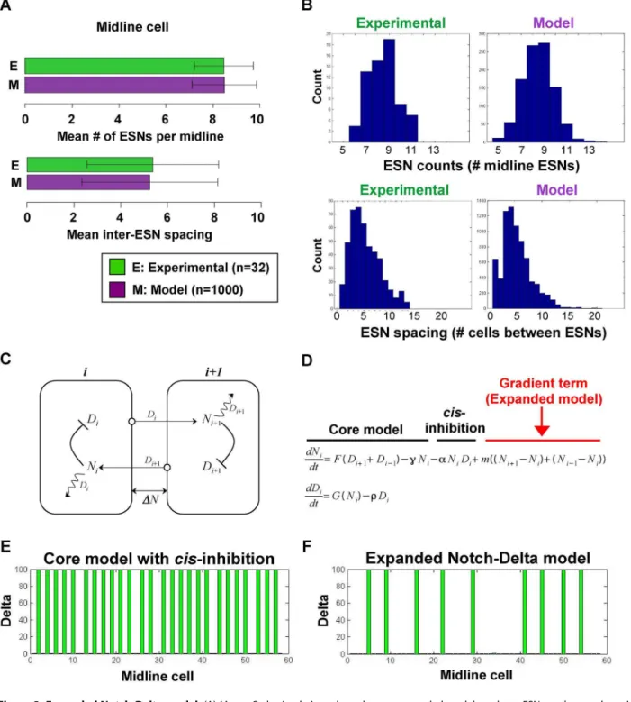
Figure 3. Expanded Notch-Delta model.(A) Monte Carlo simulations show that our expanded model produces ESN numbers and spacings that match with experimentally determined values. (B) The distributions for the number and spacing of ESNs, including the minimum/maximum and variances of the distributions, are all very similar between model and experiment. For the top graphs, the y-axis shows the number of midlines with the given number of ESNs. For the bottom graphs, the y-axis shows the number of times a given ESN spacing occurs. (C) Schematic showing the intra- and inter-cellular interactions between Notch and Delta. The squiggle arrow representscis-inhibition of Notch by Delta. Note that for clarity only two cells are shown, but the interactions extend over a linear array of cells. (D) The general form of the ordinary differential equations of our expanded model for Celli, with addition of a Notch activity gradient term indicated in red. (E–F) Shown are the equilibrium values of Delta after a typical run of our expanded model in comparison with the original core model [12,20].
An expanded Notch-Delta model exhibiting long-range ESN patterning
With this quantitative experimental data in hand, we began drafting a Notch-Delta mathematical model that could adequately explain the patterning of midline ESNs inCiona. We began with a linear array ofCcells representing a single midline at a fixed time point. As mentioned, we did not notice any obvious differences between the dorsal and ventral midlines at the larval stage (see Figure S1), so our model is appropriate for modeling either midline. Future models will modify this static array into a dynamic array that includes cell division. This 1-D model could also be easily expanded to a 2-D array for modeling planar systems such as the proneural clusters inDrosophila[5,12,20,30].
Consistent with previous minimal models, each cell tracks the activity of just two biochemical species, Delta (D) and Notch (N) or some closely affiliated biochemical species, such as a transcription factor directly linked to these primary proteins. Note that because our model can be applied to other biochemical and physical systems, when we present the differential equations of our model below, we will denote the Delta and Notch species more generally asxandy, respectively. As discussed in the original Monk model [20],ycould be taken to represent the quantity of activated Notch (i.e., Notch ICD) in the cell; or it could be taken to stand for the quantity of downstream Hes TF in the cell. In addition, since the Notch-SuH-Hes cascade is linear and exhibits bistability (i.e., there are only one of two stable states for each node - either all "ON’’ or all "OFF’’), we can regard the states of Notch, SuH and Hes as equivalent, and can therefore consider any of these or all of these lumped together as the variable y [52]. Analogously, since we know that the bHLH proneural genes are expressed in a linear cascade and are upstream of Delta [34], x could represent the quantity of membrane-bound Delta in the cell or could incorporate the activity of the upstream proneural TFs [52].
Figure 3C shows a schematic of our model for the interaction between neighboring cells. All the cells in the linear array interact with their nearest neighbors with the exception of the end cells. The model localizes x inside the cell or expressed on the cell surface to signal only the neighboring cells. It is repressed internally by y and activates neighboring cells to stimulate production ofy. The speciesxalso catalyzes thecis-inhibition of yinside the same cell. The production ofydepends on the activity ofxin the neighboring cells. Both species have linear decay terms based on the half-lives of Notch, y, and Delta, x. Finally, we include a communication term foryto neighboring cells based on the gradient in activity of active Notch or a related biochemical species between the cells. The addition of this gradient term is the primary distinction of our model from previous Notch-Delta models. In earlier models, interactions are exclusively with neighboring cells, which restricts the patterning to primarily alternating on and off states, while our model by including a Notch activity gradient can simulate larger cell spacings, which match that found inCionaand in other analogous Notch-Delta systems [7,30,37]. Although the exact mechanism of long-range commu-nication is currently unknown in Ciona, we favor a nearest-neighbor Notch gradient term versus other possibilities based on our current biological knowledge of Notch-Delta signaling in the CionaPNS (see Discussion).
All of the above interactions represent the core conserved interactions of Notch-Delta signaling and are supported by extensive experimental evidence [4,5,10,53]. Let xi and yi be the activity levels of Delta and Notch in celli, respectively, then the dynamics for the model described above is given by the following system of differential equations:
dxi dt ~
a
1zk1y n1 i
{bxi, ð1Þ
dyi
dt~{axiyiz
b(xi{1zxiz1)n2 1zk2(xi{1zxiz1)n2
{cyi
zm(yi{1zyiz1{2yi), i~1,:::,C:
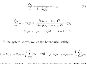
In the system above, we let the boundaries satisfy:
x0~xCz1~xave~ 1
C
XC
i~1
xi and y0~yCz1~yave~ 1
C
XC
i~1 yi,
wherexave andyave are the average activity levels of Delta and Notch over the entire array of cells. Clearly alternate boundary conditions could be considered, although other common boundary conditions such as zero or periodic boundary conditions are not appropriate for modeling theCionamidline.
The functions and the parameters in the model are common in biochemical control models [12,20,25,54]. The essential form of each function is the same as those found for earlier minimal Notch-Delta models [12,20] (Figure 3D). A full explanation of each of these functions and parameters can be found in Materials and Methods, but here we briefly mention the functions and parameters that are immediately relevant for our analysis. The first term on the RHS of theyequation representscis-inhibition byx. The parametersband care the linear decay rates of Delta and Notch or a related biochemical species, respectively. Because our biochemical species do not distinguish between mRNA and protein levels, we may take them as representing mRNA and/or protein decay rates. The last term in theyequation is the linear gradient term representing long-range communication. This cell-to-cell gradient term could result from bound Notch molecules self-signaling to create a gradient-like pattern of activity. It could be the result of another signaling biochemical closely aligned with Notch, but not necessarily bound so strongly to the membrane. From a modeling perspective this gradient form of nearest neighbor communication is the simplest mechanism of long-range patterning and makes a good first order approximation to the kinetic interactions of this signaling pathway. For the remainder of the article, we will refer toxiasDiandyiasNito associate the model state variables with the Delta (D) and Notch (N) pathways.
Monte Carlo simulation of expanded model reproduces sensory neuron pattern inCiona
When there was sufficient spacing between cells with high levels ofD, then we observed later development of cells with high levels ofDin the intervening area of cells. These later developing cells arose from two distinct dynamical behaviors. In one case there were sufficiently low levels ofN far from the ones with high levels ofD, resulting in the smooth development of an intervening cell with a high level ofD. This case was most common early in the simulation. In the second case, the levels ofDandNoscillated in the regions between stable areas of highD, with the amplitude of the oscillations appearing to increase with increased ESN spacing. With enough spacing, the oscillations increased until a threshold was crossed, allowing the development of another cell with a high level ofD.
Because of the random initial conditions, different patterns of cells with high D levels arose. The spacings in these patterns depended strongly on the parameter values; however, after sufficient time a stable pattern emerged. A representative example is shown in Figure 3F. Note that spacings of more than two cells cannot be achieved with either the original Monk model [20] nor the model incorporatingcis-inhibition [12] (Figure 3E).
To determine if our model could explain the ESN pattern along the Ciona midline, we ran a Monte Carlo simulation with M= 1000 runs over t= 4000 time steps for each run, and compared the number, spacing, and distribution of high Delta-expressing cells with that of the ESNs from wild-type embryos. Our simulations used the parameter values listed in Table 1.
The parameters were chosen for the following properties. The value forC, the number of cells, was chosen to match the average number of midline cells from our experiments. The parametersa, k1,k2,a, andbwere fairly arbitrary, although they were chosen based on our knowledge of similar biochemical control models from previous work [12,20,25,54]. As off-diagonal elements, these parameters should not be as significant to the behavior of the system as the other parameters (though theD-mediated decaya could be an important parameter when considering the effect of modulatingcis-inhibition, as in a previous study [12]). The most significant parameters for the switching behavior are the parametersn1 andn2, the Hill coefficients. These are chosen be be greater than one, but not too large to be biologically relevant. The decay ratesbandcalong with the gradient parametermare very significant as we will see in the bifurcation analysis. In particular, c will be important when we consider the effect of microRNA-mediated regulation of Notch signaling. For these simulations,cwas adjusted so that the average number of high-Delta cells over the 1000 runs closely matched the number of ESNs from wild-type experiments. Since Delta is an epidermal sensory neuron marker [34], throughout the text we will refer to high-Delta cells and ESNs interchangeably.
Figure 3F shows the end results of a typical run, with Movies S1 and S2 showing the dynamics of two separate runs starting with random low initial conditions for both Delta and Notch. Both movies show the appearance of new ESNs in regions where the spacing between existing ESNs is large. In movie S1, the levels of Notch and Delta settle into a very stable equilibrium; while in movie S2, the levels of Notch in the cells between the ESNs at Cells 27 and 39 show distinct stable oscillations. Figure 3A–B
shows the statistics for the number and distribution of ESNs and inter-ESN spacing from 1000 runs. While agreement between the average number of ESNs predicted by the model and experimen-tally observed in larvae is expected, surprisingly the distribution of ESNs and the average ESN spacing matched very well with experimental observations. The majority of runs in our Monte Carlo simulations produced between 6 and 11 ESNs, with a peak of 9 ESNs, matching experimental observations. There were some instances of outliers on either side in our simulations, although if we were able to quantify an equivalent number of embryos (M~1000), we might expect some experimental outliers as well. Similarly, the ESN spacing in our simulations matched experi-mental observations, with the frequency histograms following an identical gamma distribution with a peak at 4 cells and dropping off after 13 cells. There were a few rare outliers where ESN spacing exceeded 13 cells. When we analyzed these outliers more closely, we noticed that these large spacings were flanked on at least one side by two closely ESNs (Figure S2). These closely spaced ESNs likely stabilize the cells within the large-spacing valley. This is in agreement with our experiments showing that cases of high inter-ESN spacing were flanked on at least one side by consecutive ESNs with tight spacing (Figure S2). Finally, we note that our model has a disproportionate number of one-cell spacings compared with experimental observations. This is likely due to the intense stability of the high-Delta cells and the strong effect of lateral inhibition in our model.
We chose our Hill coefficients n1 and n2 based on our knowledge of previous biochemical control models [12,20], which produced the reasonable fits seen in Figure 3A–B. However, we know that changing the coefficients,n1andn2, affects the lateral inhibition and induction of immediately neighboring cells and results in differing distributions of cell spacing. Simulations with n1~3 and n2~3 produced significantly broader distributions (similar means, but a much larger variance), while n1~5 and n2~3produced a much narrower distribution (similar mean with a smaller variance). Our modeling experiments suggest that increases, especially inn1, would produce more two-cell spacings at the expense of one-cell spacings as suggested in the experiments. However, since Figure 3A–B shows our model adequately represents the experiments, we chose to center our studies around the casen1~4andn2~2.
Stability analysis explains midline ESN patterning A stability analysis is used to determine equilibrium states of a system and the change in behavior of a system as the parameter values vary. This analysis is important because it allows us to determine the possible ESN patterns that can be produced from our model, and to rigorously determine if our model can really explain the biology. We therefore designed programs to help numerically find equilibria and allow the stability analysis of the equilibria. The stability analysis uses the Jacobian matrix analytically derived from linearizing the system (1) (see Materials and Methods).
There is a unique homogeneous equilibrium for system (1). Related systems [20,42–44] have been analyzed in terms of the stability of the homogeneous equilibrium, showing the existence of
Table 1.Parameters used for the Monte Carlo simulations.
C~58 a~10 k1~10 n1~4 b~0:1
a~1:2 b~10 k2~2 n2~2 c~0:069 m~0:1
Turing solutions. For system (1) with the parameters in Table 1, there is a homogeneous equilibrium with xe~0:1418 and ye~2:897, which is unstable with multiple positive eigenvalues.
Since the experimental studies do not suggest a periodic pattern, we did not explore Turing solutions. Our primary interest was the behavior of the many inhomogeneous equilibria.
The Monte Carlo simulations showed the variety and large number of possible stable equilibria for model (1). This model can easily reproduce the stable alternating pattern of the previous Monk [20] and Elowitz [12] models. These models are very similar to (1) withm= 0 anda= 0, respectively; however, non-zero values ofm and aallow the richer stable patterns shown in the Monte Carlo simulations. From the many equilibria for this system we chose to systematically explore the stability of the system with different spacings of high D levels. The numerical observations showed decreased stability of the cells some distance from the cells with high D levels, so we wanted to explore the nature of any bifurcations leading to limits on the spacing of the cells. Below we present the stability analysis for different ESN spacings, giving information about the dominant eigenvalues and commenting more about the observed eigenvalue structure. The parameters we use in this analysis come from Table 1. In biological terms, the eigenvalues and eigenvectors tell us the differentiation state of each of the midline cells. Roughly speaking, if a cell aligns with an eigenvector associated with the most negative eigenvalues, then it is stable and has fully differentiated into an ESN. The cells that align with the largest components of the eigenvectors associated with eigenvalues with positive real part are unstable and remain bipotent.
To help minimize the effects of the boundary, we varied the number of cells in our simulations to be as close as possible to C~58(which is the average number of midline cells found in all of our experiments), while maintaining symmetry at the bound-aries. Suppose two consecutive ESNs are Celliand Cellj, then defineP~j{i(1 ESN andP{1epidermal cells). We numerically find the equilibrium of (1) for each value ofP. From the linearized form computed in Materials and Methods, we can readily find the eigenvalues and eigenvectors for this system. Table 2 summarizes the results of different spacings using the parameters from Table 1 and shows the dominant eigenvalues of the system.
The linear stability analysis of (1) with the parameters from Table 1 and the spacings and numbers of cells from Table 2 gives a better understanding of this system. The overall stability of system (1) is determined by the real part of the dominant eigenvalue, lmax, with this system being asymptotically stable if
and only if Re(lmax)v0. However, this is a high-dimensional system, and different components of the model behave differently near an equilibrium based on its structure. The time-series local behavior of different components vary more or less depending on their location, and their fate can be understood by careful examination of the eigenvector associated with specific eigenval-ues.
With MatLab we computed all eigenvalues and eigenvectors for each of the cases in Table 2. In every case we had the smallest eigenvaluelmin&{120with a multiplicity matching the number of cells with high levels ofD. By examining the corresponding eigenvectors, we found the largest components centered on the highestD(lowestN) values. (Note that because of the scaling, the Dcomponents of the eigenvectors are much smaller than theN components, so we compared only relative size withinD or N components.) Each of the eigenvectors associated with one of the eigenvalues, lmin, had a large D component and a large N component at one of the ESN positions with all other components at least four magnitudes of order smaller. This agrees with our observation that the model produces extremely stable regions near cells with high levels ofD,i.e., differentiated ESNs.
The real part of the dominant eigenvalue,lmax, becomes larger as the spacing, P, increases. This correlates to the decreasing stability of the levels of Dand N as the spacing increases. The multiplicity oflmaxmatches the number of interspacings between cells with highD. When examining the particular components of the corresponding eigenvectors, the patterns were more complex, spreading across several interspacings. However, the maximumD -component occurred near the center of the interspacings with the maximumN-components flanking either side of the maximumD. This is in line with the observation that the next highest D -component always occurs near the middle of our cells with high levels ofD, while the flanking cells show the highestNresponses in agreement with Notch being highest in cells neighboring a cell with high Delta.
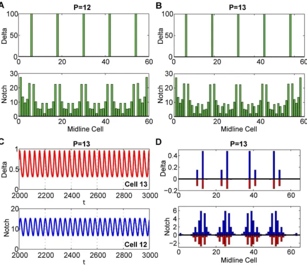
As P increases, the real part of lmax changes signs between P~12andP~13, giving a Hopf bifurcation. Figure 4A–B shows the equilibrium state of the system at P~12 and 13, and the simulations show distinct oscillations. From Table 2, any simulation withP~12would show damped oscillations with the solution settling to the equilibrium. The eigenvalue forP~13has a frequency of 0.1877, which implies a period, T&33:5.
Figure 4C–D shows the oscillatory solutions from a simulation withP~13, and the period of oscillation agrees with the frequency of lmax. The eigenvectors of lmax withP~13 show a structure
Table 2.Different spacings of highDgiven byP.
P C lmax nl Stability
5 58 {0:0933 11 Stable
6 59 {0:0775 9 Stable
7 54 {0:0472 7 Stable
8 55 {0:0189+0:1258i 12 Stable
9 61 {0:0118+0:1608i 12 Stable
10 59 {0:0069+0:1777i 10 Stable
11 53 {0:0068+0:1820i 8 Stable
12 59 {0:0057+0:1837i 8 Stable
13 63 0:0014+0:1877i 8 Unstable
Cgives the number of cells in the array.lmaxgives the dominant eigenvalue, andnlgives the multiplicity of the dominant eigenvalue.
very similar to the graph in Figure 4D, where variation for each cell from its equilibrium is displayed. The variation inD is very small (about 1%) compared to the size of the high Delta cells, while the oscillations in N are quite substantial relative to the equilibrium Notch levels, especially in the cells flanking the cell, which has the greatest variation in D near the middle of the interspacing region. This example with P~13 has an unstable equilibrium, but its oscillations are insufficient in magnitude to cross a threshold and pass to a different equilibrium with high Delta cells between the ones shown in Figure 4B. We note that slightly different initial conditions away from the equilibrium will cause new ESNs to arise, indicating that the basin of attraction for theP~13equilibrium shown is quite small.
Once P§14, our numerical algorithms cannot find an equilibrium solution to linearize around and any simulation results in new ESNs appearing, indicating the P§14 spacings are too unstable when evenly spaced. Thus, our model suggests that when the number of cells between ESNs becomes too large, then new ESNs appear in between. Importantly, in agreement with this bifurcation analysis on P, our wild type experiments show a maximum spacing of 13 cells between ESNs. This suggests that if the midline cells divide and the spacing becomes greater than 13, the instability of such a state will cause a new ESN to appear. Also
recall that with our parameter values the spacing mean and distribution matched the wild type experiments. Thus, our experimental results are in harmony with our numerical analysis of the spacing,P.
The analysis above examines discrete changes in the spacing,P. We next chose to explore continuous changes with the gradient parameterm. For these studies we setP~10,C~59, and all other parameters from Table 1 except form. From the analysis above we know that instabilities should cause an ESN to appear midway between and create aP~5pattern. Our interest is to determine something about the dynamics of change from a larger spacing, P~10, to a smaller spacing,P~5.
Decreasingmin essence shortens the effective distance of Notch signaling. As noted before, when m~0, the Monk model only produces an alternating pattern of highDandNwith no spacings larger than two and most being one. Thus, we expect the stability of theP~10 pattern to be lost as m decreases. We studied the linear stability of the P~10 pattern as m ranged from 0.2 to 0.08845. At the ESNs, where xi is high, i~5,15,:::,45,55, the
smallest eigenvalue is lmin&{120, making this region of the cellular array extremely stable. The maximum eigenvalue, lmax has its eigenvector centered between the cells with high D. Figure 5A shows the variation in the real part oflmaxasmvaries.
Figure 4. Stability analysis of the ESN spacing,P. (A–B) The top graphs show the equilibrium values for the Delta and Notch levels. (C–D) The bottom graphs examine the unstable caseP~13and show the time varying oscillations (left) of Cell 13 forDand Cell 12 forNand the variation from the equilibrium for all cells (right).
When we decreasemtom&0:08985, there is a Hopf bifurcation
(verified with Auto in XPPAUT), introducing oscillations in cellular activity levels, xi and yi. The maximal oscillations in xi
occur in the middle cells, i~10,20,:::,50, while the maximal
oscillations inyioccur in the adjacent cells, e.g., Cells 9 and 11. Figure 5B–C shows the equilibrium levels forx10 andy9, and the maximum and minimum of the oscillating levels after the Hopf bifurcation. As is typical of a Hopf bifurcation, these oscillations increase in amplitude away from the Hopf point.
Asmdecreases further to approximately 0.0885, the instabilities are sufficient that the solution leaves the basin of attraction for the P~10equilibrium. The result is that the solution converges to the very stable pattern where xi is high at i~5,10,15,:::,50,55,
resembling theP~5equilibrium. The maximum eigenvalue for this solution islmax~{0:09, producing a very stable equilibrium.
We note that the basin of attraction for this solution is significantly larger than the basin of attraction for theP~10case. Figure 5B–C shows the increase of bothDandN asmdecreases. It appears as though some threshold is reached, which results inx10 approach-ing 100 andy10 going to very low levels quickly. It is not clear if this transition is smooth and very rapid or if some saddle node bifurcation is occurring. At this time the specific type of bifurcation moving from the P~10 to the P~5 spacing has not been determined and needs further analysis.
Finally, we analyzed the change in behavior of the system as we increased the Notch decay rate parameter, c. We began with a constant spacing of P~10 cells and the corresponding value of C~59 from Table 2, with all other parameters from Table 1. Starting with a low value ofc~0:04, we increased the value ofc
with a step size initially of 0.01. As we stepped fromc~0:11 to c~0:12, a significant change in the system occurred whereby new
ESNs appeared halfway between existing ESNs, similar to what occurs when we decrease m. Through repeating this stepping process with decreasing step sizes, we determined the exact value of this critical value of c to be ccritical~0:112607. With every
iteration of this process, we kept track of the minimum and maximum eigenvalues and associated eigenvectors (Figure 6A), as well as the equilibrium values ofDandN (Figure 6B).
As in the case ofm, analysis of the min/max eigenvalues and associated eigenvectors revealed that the existing ESNs (e.g., Cell 5) are highly stable, while the middle intervening cells (e.g. Cell 10) are in regions of lower stability. However, unlike withm, the levels ofy9andx10do not exhibit oscillations as we approach the critical value ccritical~0:112607 (Figure 6B). The real part of the
maximum eigenvalue lmax remains negative as we vary c, indicating that there is no Hopf bifurcation (Figure 6A). At ccritical, the system moves out of the basin of attraction forP~10 and converges to a new stable pattern with smaller spacings resembling theP~5equilibrium (Figure 6C–D). The behavior in Figure 6B is similar to a saddle node bifurcation, but a more detailed analysis is required. As we decreasecback toc~0:04, the
system remains in the new equilibrium, indicating that this equilibrium is very stable and has a very large basin of attraction. In biological terms, we may interpret this hysteresis effect as the newly formed neurons have committed to their new state and will not easily revert back to being bipotent.
Significantly, our analysis shows that increasing c beyond a critical value can produce new cells with high levels ofD, which demonstrates that, based on our model, increasing the Notch decay rate can produce new ESNs. This directly relates to our consideration of the influence of microRNAs on Notch decay rates and ectopic ESN formation in the last two sections.
Parameter sensitivity analysis
In the study of any model, it is important to determine which parameters have the greatest effects on the system. Our model is a high dimensional, nonlinear model with a large number of
equilibria, so one would expect that the sensitivity of the model depends on the region of parameter space where the analysis is performed. Some equilibria will have large basins of attraction and will therefore be very robust to parameter changes, while other equilibria will have smaller basins of attractions and will be more sensitive. For this parameter sensitivity analysis, we examine variations of+10% in each of the parameters for our case where C~59andP~10, using the other parameter values from Table 1. This equilibrium is associated with a pattern of six neurons with 9 cells between each neuron, and we chose to focus on this equilibrium since this was the mean spacing and neuron count found experimentally and therefore should give us a general idea as to which parameters have a greater effect on our system. We established that the equilibrium for this system was stable and found the eigenvalues.
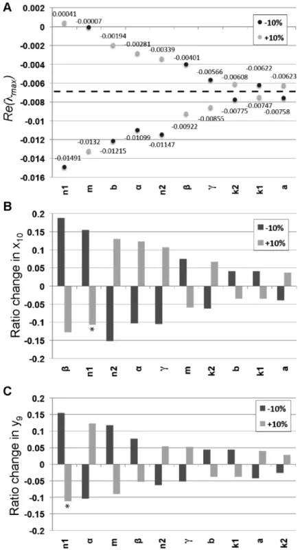
One measure for the sensitivity is the change in the value of the real part of the maximum eigenvalue. With the base parameters, we foundRe(lmax)~{0:00688. Figure 7A shows that increasing
the coefficient of the negative feedback function, n1, has the greatest effect, and even results in the system going through a Hopf bifurcation. Decreasing the parameter m has the next largest effect, which is not too surprising given that its parameter value is
close to the Hopf bifurcation for that parameter. As we would expect, the parameters,a,k1 andk2 have minimal effect on the eigenvalues, while the other parameters have more varied effects increasing or decreasing the stability. Figure 7A shows the effects of variations of+10% for all the parameters on the real part of the largest eigenvalue,lmax.
Our study shows that in the case whereC~59andP~10, the greatest instability lies in the center between two ESNs. This can be visualized by examining the eigenvector for Re(lmax). The largest level ofxaway from the ESNs occurs atx10,x20,…x50(see Figure 6C). The least stable levels ofyoccur in the neighboring cells, such asy9 and y11 (see Figure 6C). Figure 7B–C provide information on how much a variation of +10% in a given parameter shifts the equilibrium values at x10 and y9, where changes in amplitude are observed to be the largest. When a shift becomes sufficiently large atx10and a threshold is crossed, a new ESN forms in this location, completely changing the equilibrium values forxandy. Figure 7 shows that a description of parameter sensitivity for this system depends on the measure that is employed. Clearly, this system is most sensitive to the negative feedback coefficient,n1. However, the Hill coefficients relate to the degree of cooperativity for binding between Notch and Delta,
Figure 6. Stability analysis of the parameterª. (A)Re(lmax)forP~10(blue) andP~5(red) ascvaries. (B) Equilibrium levels of Delta (top) and Notch (bottom) for our casesP~10(blue) andP~5(red) ascvaries. Note that Delta is shown as a semilog-y plot to show the change in Delta. (C–D) Equilibrium levels for Delta and Notch across all midline cells as we crossccritical~0:112607.
Figure 7. Parameter sensitivity analysis.(A) The values ofRe(lmax)are shown for all the parameters of the model with variations of+10% in each of the parameters. The ordering of the parameters shows which parameters had the largest increase in the eigenvalues for either a+10% change with the largest on the left. The dotted line indicates the value ofRe(lmax)for the original set of parameters used in Table 1. (B) The change in equilibrium value forx10after+10% change in parameter values. The y-axis shows the ratio change of the equilibrium with the new parameter value
divided by the original equilibrium valuex10~0:4405. The ordering of the parameters shows which parameters had the largest increase in the
magnitude ofx10for either a+10% change with the largest increase on the left. Since the equilibrium is unstable forn1~4:4,x10 oscillates 17%
above and 14% below the equilibrium marked with a. (C) The change in equilibrium value fory
9after+10% change in parameter values. The y-axis
shows the ratio change of the equilibrium with the new parameter value divided by the original equilibrium valuey9~8:695. The ordering of the parameters shows which parameters had the largest increase in the magnitude ofy9for either a+10% change with the largest increase on the left.
Since the equilibrium is unstable forn1~4:4,y9oscillates 13% above and 10% below the equilibrium marked with a.
which are intrinsic properties of the proteins not likely to change over development. As we alluded to before though, decreasingn1 broadens the ESN count and spacing distributions, while increasing n1 narrows the distributions (Figure S3). We found that a 10% change in m caused a *20–25% shift in the ESN spacing and count distributions, suggesting that the system is indeed sensitive to this parameter (Figure S3). The least significant parameters are the kinetic constants, a, k1, and k2. A 10% variation in k1 results in a *10% change in ESN count and spacing distributions (Figure S3). The robustness of this model to variations in most of the parameters allows reasonable stability for patterning of ESNs, while providing flexibility to produce novel patterns when new adaptations are necessary, such as a need for more or less dense ESNs.
Incorporation of miR-124 regulation of Notch signaling into the expanded model
We previously showed that the microRNA miR-124 is expressed in the larval midline ESNs of Ciona intestinalis[33,46]. We demonstrated that miR-124 is activated by proneural bHLH genes and negatively regulates Notch signaling by downregulating Notch and all three Hes genes [33,34] through binding to canonical target sites in the corresponding transcript30UTRs[33]. Mis-expression of miR-124 along the entire epidermal midline increases the number of midline ESNs presumably because of ectopic suppression of Notch signaling [33], although a detailed quantitative analysis was not performed.
Here we generated transgenic embryos using this same miR-124 construct from our previous studies (Epi::miR-124) [33,46]. We electroporated increasing amounts of the transgene into Ciona embryos (10mg,20mg, or30mg; which we denote as Epi::miR-124+
10, Epi::miR-124+20, or Epi::miR-124+30, respectively). In each case, we quantified the number and spacing of ESNs at 22 hours post-fertilization, and compared these results to control wild-type 22 hr embryos. We used immunohistochemistry to detect ESN cilia with an anti-acetylated tubulin antibody, and visualized the midlines with either an Ash or Delta fluorescent transgene reporter. We performed each experiment with independent biological replicates, and quantified a total of 17, 19 and 20 embryos for the miR-124+10, miR-124+20 and miR-124+30 experiments, respectively. We only quantified embryos for which we could clearly perform cell counts for both the dorsal and ventral midlines; since miR-124 overexpression produces kinked or twirled phenotypes that make counting difficult, we were not able to quantitate as many embryos as in the wild-type experiment.
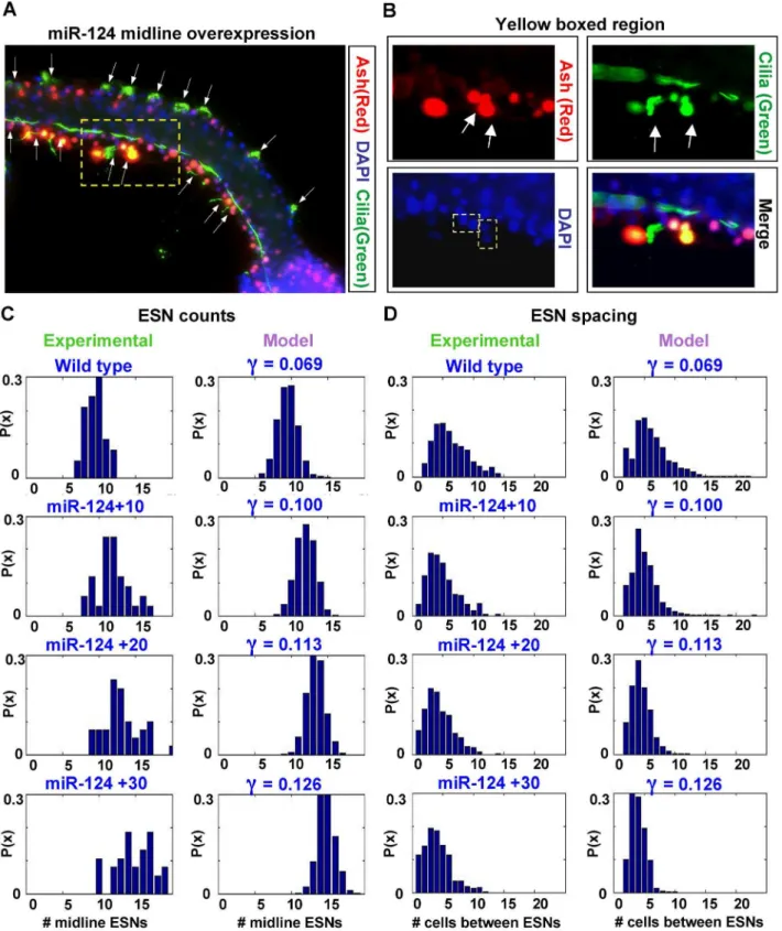
Figure 8A–B shows a representative embryo, and the results of our Epi::miR-124 titration experiments are shown in Figure 8C– D. As we increased the amount of the miR-124 transgene electroporated into embryos, the mean number of ESNs per midline increased with a corresponding decrease in the mean ESN spacing. Note that the mean number of midline cells was very similar between the experiments (mean = 57.7, 57.0, 57.3, 58.9 in wild-type, +10,+20 and +30, respectively), indicating that miR-124 overexpression did not affect the number of midline cell divisions during development (see Figure S1). The largest difference occurred between wild-type and miR-124+10 embryos (difference in mean ESN counts = 2.44; difference in mean ESN spacing =22.44); subsequent increases in miR-124 concentration had a linear effect on the number and spacing of ESNs (average difference in mean ESN counts = 1.45; average difference in mean ESN spacing =21.43). Comparison of ESN count and spacing distributions and the associated minimum/maximum values among the different miR-124 concentrations also showed a shift
towards an increasing number of ESNs per midline and decreasing inter-ESN spacing. In particular, the number of zero-spacing cases (i.e., adjacent ESNs) increased as the concentration of miR-124 was increased. A magnified region of the embryo in Figure 8A shows one such case of adjacent ESNs (Figure 8B), which we did not observe in wild-type embryos. This suggests that when expressed at high levels, miR-124 is able to mitigate the effect of lateral inhibition.
Since miR-124 downregulates Notch and Hes by base pairing to their transcript30UTRsand likely mediating decay at the post-transcriptional level [33,55–58], we proposed that miR-124 regulation of Notch/Hes could be modeled into the Notch decay rate, c. An increase in miR-124 concentration would thus be reflected in our model by an increase in the value forc. To test this hypothesis, we began with the c value from our wild-type simulations (c~0:069) and ran Monte Carlo simulations
(M = 1000) continuously increasing the value of c to see if we could match the average number and spacing of high-Delta cells with the number of ESNs in our miR-124 titrations. In agreement with our experiments, we showed in the previous section that continuously increasingceventually resulted in the formation of new neurons, suggesting that production of extra midline ESNs could be explained by an increase in the Notch decay rate. Indeed, as we continued to increase c, the average number of ESNs continually increased. Eventually, we found values for which both the mean ESN counts and inter-ESN spacing closely matched the observed values in each of the miR-124 titration experiments (c~0:100for miR-124+10;c~0:113for+20;c~0:126for+30,
Figure 8C–D). The marginal increase incis greatest from wild-type to miR-124+10 embryos, correlating with the high marginal increase of ESN counts between these two samples. Importantly, the distributions of ESN counts and spacings closely fit the experiments, with the model also showing corresponding shifts in the distributions upon increasing gamma values (Figure 8C–D). The variance of the model is smaller than the corresponding miR-124 experiments, even though in the wild-type case the variances were similar between model and experiment. However, overall the model agrees very well with the miR-124 experiments, even more surprising given the fact that we can mimic the experimental ESN patterns with the tuning of just a single parameter. Coupled with extensive biological support [33,55–58], we conclude that our model can accurately incorporate the experimental effect of miR-124 into the Notch decay rate term.
Evidence that expanded model explains regulation and patterning in sensory cell types across bilaterians
Notch signaling regulates the specification and patterning of sensory cell types not just in Ciona, but throughout metazoans (reviewed by [5,10,26,53]). Examples of processes regulated by Notch-Delta signaling include the mechanosensory bristles (macrochaetes and microchaetes) of D. melanogaster [30,31]; the inear ear hair cells of zebrafish [59–61], chick [41,62], and mouse [41,63,64]; and the multiciliated cells derived from the respiratory airway epithelium in humans [65,66]. Interestingly, the sparse patterning in Ciona appears also to be found in other animals [7,30,31,35,37], suggesting that long-range Notch-Delta signaling is also conserved.
Figure 8. The microRNA miR-124 modulates the Notch decay rate. (A) Representative embryo for miR-124 titration experiments. (B) Magnified region of the embryo in (A) shows adjacent ESNs; DAPI staining shows pairs of small nuclei belonging to the ESN pairs. (C–D) Comparison of the distribution of ESN counts and spacing between miR-124 titration experiments and our model. Based on this data and our previous results [33,34], we propose that the Notch decay rate,c, is modulated by miR-124.
that miR-124 rarely targets Notch pathway genes in other organisms [33]. Interestingly though, miR-9 inDrosophilaappears to regulate Notch signaling in a somewhat analogous fashion [70], suggesting that different organisms deploy different miRNAs to
regulate Notch signaling [33]. This would suggest that incorporation of miRNA function into the Notch decay term of our expanded model may be relevant for other systems.
Figure 9. Canonical target sites for miRNAs expressed in sensory cell types throughout bilaterians.Notch signaling regulates the differentiation and patterning of each of the sensory cell types shown. Sensory cell expression for each of the miRNAs listed was shown previously (see text for references). miRNA canonical target sites in the30UTRs of Notch and Hes homologs were found using our previously described target prediction algorithm [33]. Some of these targets have been experimentally verified (V) (human: [65]; sea squirt: [33]; fruit fly: [9]). InDrosophila, miR-2, miR-6 and miR-7 overexpression (O) have all been previously shown to cause a phenotype indicative of suppressed Notch signaling activity and loss of lateral inhibition, such as increased density or clustering of microchaetes [9]. In human airway epithelial tissue, knockdown (K) of miR-449 has been shown to cause a decreased rate of ciliated cells indicative of Notch signaling gain-of-function [65].
To determine if this might be the case, we first examined the literature to identify sensory neuron-expressed miRNAs in Drosophila, zebrafish, mouse, and human. For miR-124, we only found one study in mice where weak miR-124 expression was reported in the vertebrate inner ear [67]. However, many other miRNAs are highly expressed during mouse inner ear develop-ment [67,71,72]. In other bilaterians, different miRNAs are expressed in these sensory cells, with no obvious conservation of particular miRNA expression (Drosophila: [9,73,74], zebrafish: [71], human [65,66]).
We then bioinformatically searched for canonical target sites of these sensory miRNAs in the30UTRsof Notch pathway genes in these animals using a target prediction program we developed previously [33]. Through this, we discovered the presence of predicted target sites in the primary Notch receptor (Notch1) among vertebrates, as well as target sites for other Notch homologs in zebrafish and mouse (Figure 9). In agreement with our hypothesis, we found Notch1 target sites for different sensory miRNAs in each of the different organisms (miR-124 in Ciona, miR-15a in zebrafish, miR-30b,2100,2125b,2133a,2182 and 183 in mouse; and miR-34 and miR-449 in human airway epithelium). Among these, miR-34 and miR-449 targeting of Notch in human airway epithelial tissue has been experimentally verified [65]. We did not find any target sites for Notch in Drosophila, suggesting that such sensory miRNA regulation of the Notch receptor did not evolve until at least after ecdysozoans.
In agreement with previous reports, we also observed sensory miRNA target sites within many Hes homologs in Drosophila [9,75]. However, whereas inDrosophilaandCionaalmost all of the Hes homologs have target sites, we observed that in vertebrates predicted targeting of Hes is much more restricted (Figure 9). This may be explained by the fact that predicted targeting of the Notch receptor appears to be much more extensive in chordates (Figure 9). Since the Notch receptor is the initial effector of Notch signaling, miRNA-mediated suppression of Notch would relieve the need to target all of the downstream Hes factors. Another possible explanation is that the other Hes factors are not expressed in the sensory cells of vertebrates, and therefore their targeting by sensory miRNAs is not needed. Indeed, among the many Hes homologs in mice, only Hes1 and Hes5 are expressed in inner ear cells, of which Hes1 is the more highly expressed factor [27,76].
Finally, we note that although inC. elegansthere is no published evidence of Notch signaling regulating sensory neuron formation, the Notch homolog LIN-12 regulates the formation of some of the adjacent interneurons that relay signals from the sensory neurons [77]. Recent evidence suggests that the miR-51-56 family is ubiquitously expressed among neurons inC. elegans[78], and we bioinformatically found a canonical target site for this family of miRNAs in the LIN-1230UTR. Although in this work we focused on sensory cell types in other organisms, since they are most analogous to the epidermal sensory neurons ofCiona, but it would be interesting to explore miRNA regulation of Notch signaling in other cell types.
Discussion
Our experimental results inCiona and previous related studies motivate an expanded Notch-Delta model
Previous Notch-Delta models [12,20–24] were based on early Notch signaling studies in Drosophila, Xenopus, and mouse [2], which suggested a checkerboard expression pattern whereby neighboring cells adopted alternate cell fates. This was supported by evidence in Drosophila that cells selected to become neurons activate Notch signaling in neighboring cells thereby preventing
these cells from likewise adopting a neuronal fate [5]. This led to the classic Monk model [20], which provided the foundation for later models [12,21–24].
However, more careful analysis has shown that the pattern produced by Notch-Delta signaling in some cases is not checkerboard. For example, the sensory microchaetes of the Drosophila thorax are initially formed at every other cell and prevent immediately neighboring cells from adopting a sensory fate via lateral inhibition. However, once the thorax has fully developed, these microchaetes become spaced about 4–5 cells apart. Meanwhile, the larger macrochaetes can be spaced dozens of cells apart [29,30,38]. In these cases, it has been suggested that dynamic filopodia extensions may provide a mechanism whereby the Delta ligand can activate Notch signaling in non-neighboring cells [28,30]. Other examples of experimentally observed non-checkerboard patterning include sparse patterning of bristle cells in other fly species [38]; opposing gradients of Notch versus Delta expression along the apical-basal axis in the developing retina of both mouse and zebrafish [7,37]; and gradient expression of Notch in the mouse inner ear [41]. These examples suggest the need for updated Notch-Delta models that can reproduce these non-checkerboard patterns. One such model has recently been developed for describing the sensory bristle patterning inDrosophila incorporating filopodia extensions [31]. This model requires dynamic lengthening and shortening of filopodia and incorporates data on several variables such as length of filopodia, lifetime of filopodia and sensitivity of Notch signaling to the Delta ligand specific to their experiments. More general models of juxtacrine systems have explored periodic patterning with longer wave-lengths, producing sparser patterns also [42–44].
Here, we developed an expanded Notch-Delta model that builds upon the minimal equations established first by Monk and later Elowitz and colleagues [12,20]. Our model incorporates a simple activity gradient that allows for long-range cell communi-cation through juxtacrine (cell-cell) signaling. This is actually a long-range inhibition, mediated by local juxtacrine signaling, using a linear gradient term similar to Fickian diffusive flux. As mentioned earlier, specific examples of Notch-Delta patterning inDrosophila[28–30] and other fly species [38], as well as in the mouse inner ear [41], mouse retina [37] and zebrafish retina [37] all demonstrate that sparse or gradient neuronal patterns can arise from a field of neurocompetent cells. Unlike the model for Drosophila neuronal patterning [31], our model does not require the existence of dynamic filopodia extensions, and actually makes very few assumptions regarding the exact pattern of neurons and the underlying mechanisms responsible for neuronal patterning. Our model can produce a large number of possible equilibrium states and, although here designed for a linear array of cells, is easily adaptable to a planar field of cells. Therefore, we suggest that our model is adaptable and able to reproduce a variety of both sparse and dense spatial patterns, and should be useful for modeling other Notch-Delta systems.
This is the motivation for updating the previous Monk and Elowitz models with the addition of a Notch gradient term. For this study, we represent this long-range term as a simple activity gradient, and demonstrate that this is sufficient for explaining the patterning of ESNs inCiona. We note that this is not necessarily a diffusion term, since Notch and Delta are membrane-bound and in most cases do not produce diffusible species. We chose a linear gradient over other possibilities, such as Hill function interactions [44], because it is the simplest and most generic form, and can be applied to a wide variety of biological and physical systems without assuming anything about the underlying mechanisms of long-range com-munication. One possible mechanism of long-range communica-tion via Notch signaling inCionamay be through the proteinCi -fibrinogen, which is secreted from the tail notochord and is known to interact with Notch in theCionacentral nervous system [79].Ci -fibrinogen is similar to the -fibrinogen-like protein Scabrous, which is involved in producing large-cell bristle spacings in Drosophila [28]. We will explore this and other possibilities in future studies and will update our model accordingly.
Finally, we provide a strong mathematical foundation for our model by performing rigorous stability analyses and bifurcation analyses of the key model parameters: the neuron spacing (P), the Notch decay rate (c), and the slope of the linear gradient (m). The sensory neurons inCionaderive from bipotent precursor cells along the tail midline, which adopt either an epidermal or neuronal fate [32–34]. Our eigenvector/eigenvalue analysis for different spac-ings between neurons demonstrates that the cells committed to becoming neurons occupy regions of high stability, while epidermal precursor cells more centrally located between consec-utive neurons occupy regions of instability. These centrally located cells thus maintain their bipotent character. These cells may have very small basins of attraction for maintaining low levels of Delta and thus, are sensitive to perturbations and small changes in the parameters of the system. As we varied the parametersP,m, and c, we discovered a threshold phenomenon whereby the system increasingly loses stability to a point where it jumps to a new equilibrium with these central cells becoming neurons. Formand c, these cells exhibit a hysteresis effect and remain committed to a neuronal fate (i.e., express high levels of Delta), even if the parameters are adjusted back to their original values.
Motivation for a Notch gradient term
An early study using bothin situ hybridization and immuno-staining demonstrated an apical-to-basal gradient of Notch expression within neuroepithelial precursor cells in the dienceph-alon, telencephdienceph-alon, retina and spinal cord during chick develop-ment [36]. More recently, apical-to-basal expression gradients of Notch were also found within neuroepithelial cells in the zebrafish retina, where Notch-Delta signaling is active [37,80]. The nuclei within these neuroepithelial cells are able to migrate along the basal-apical axis, and depending on where these nuclei are within the Notch gradient, after mitosis the daughter cells either remain in their precursor state or differentiate into neurons. Although these studies were examining intra-cellular gradients, this moti-vated us to consider the possibility that Notch gradients exist between cells along the midline. Intercellular gradients induced by cell-cell signaling relays have been well-established for TGF-b family signaling [44,81], and although not yet definitely shown to cause gradient patterns, signaling relays also exist in the context of Notch-Delta signaling through Notch activation of secondary relay ligands such as Jagged/Serrate [2,41].
We found here (Figure S4) and also in previous studies [32–34] that Delta expression is restricted to the presumptive ESNs and is not expressed in the other midline cells, therefore a
Delta-mediated gradient is not appropriate. Studies of the morphology of Ciona sensory neurons found no evidence for dynamic filopodia extensions in the PNS [51], and so the Cohen model is also not appropriate [31]. Conversely, Notch is expressed in all midline cells and, therefore, could mediate long-range communication [6]. Also, from our previous experiments [33,34], we know that blocking midline Notch signaling using a dominant-negative form of the dowstream effector gene Suppressor-of-Hairless results in ectopic neuron formation along the entire midline. On the other hand, ectopic activation of Notch signaling along the entire midline through mis-expression of Delta causes a reduction in midline neuron formation and large regions without ESNs [34]. Thus, given our experimental knowledge inCionaand knowledge of long-range patterning in other systems, our current hypothesis is that the Notch signal is somehow relayed from ESN-neighboring cells to more distant cells. Therefore, the most reasonable term to add to the original Collier model, given our experimental observations, would be a Notch activity gradient. From a dynamical systems perspective, this is also the simplest form in our model that can produce distal spacing patterns. This Notch gradient may be produced through lateral induction of secondary Notch ligands as in other animals [2,41]. InCiona, it is known that Ci-fibrinogen interacts with Notch to regulate neuronal patterning in the central nervous system [79]. Given that a similar Notch ligand, Scabrous, is involved in producing long spacings in the Drosophila PNS [28], it is possible that Ci -fibrinogen may also act as a Notch ligand in the PNS as well. We will be exploring these and other possibilities in the future. Overall, the linear Notch gradient term provides a simple initial model, which explains the Notch-Delta-mediated patterning of sensory neurons inCionabased on our current biological knowledge of the CionaPNS, and motivates future experiments and updated models.
Future work and refining our model