❊♥s❛✐♦s ❊❝♦♥ô♠✐❝♦s
❊s❝♦❧❛ ❞❡
Pós✲●r❛❞✉❛çã♦
❡♠ ❊❝♦♥♦♠✐❛
❞❛ ❋✉♥❞❛çã♦
●❡t✉❧✐♦ ❱❛r❣❛s
◆◦ ✸✼✹ ■❙❙◆ ✵✶✵✹✲✽✾✶✵
❆ss❡ts✱ ▼❛r❦❡ts ❆♥❞ P♦✈❡rt② ■♥ ❇r❛③✐❧
▼❛❜❡❧ ◆❛s❝✐♠❡♥t♦✱ ▼❛r❝❡❧♦ ❈♦rt❡s ◆❡r✐✱ ❆❧❡①❛♥❞r❡ P✐♥t♦ ❞❡ ❈❛r✈❛❧❤♦✱ ❊❞✲ ✇❛r❞ ❏♦❛q✉✐♠ ❆♠❛❞❡♦
▼❛rç♦ ❞❡ ✷✵✵✵
❖s ❛rt✐❣♦s ♣✉❜❧✐❝❛❞♦s sã♦ ❞❡ ✐♥t❡✐r❛ r❡s♣♦♥s❛❜✐❧✐❞❛❞❡ ❞❡ s❡✉s ❛✉t♦r❡s✳ ❆s
♦♣✐♥✐õ❡s ♥❡❧❡s ❡♠✐t✐❞❛s ♥ã♦ ❡①♣r✐♠❡♠✱ ♥❡❝❡ss❛r✐❛♠❡♥t❡✱ ♦ ♣♦♥t♦ ❞❡ ✈✐st❛ ❞❛
❋✉♥❞❛çã♦ ●❡t✉❧✐♦ ❱❛r❣❛s✳
❊❙❈❖▲❆ ❉❊ PÓ❙✲●❘❆❉❯❆➬➹❖ ❊▼ ❊❈❖◆❖▼■❆ ❉✐r❡t♦r ●❡r❛❧✿ ❘❡♥❛t♦ ❋r❛❣❡❧❧✐ ❈❛r❞♦s♦
❉✐r❡t♦r ❞❡ ❊♥s✐♥♦✿ ▲✉✐s ❍❡♥r✐q✉❡ ❇❡rt♦❧✐♥♦ ❇r❛✐❞♦ ❉✐r❡t♦r ❞❡ P❡sq✉✐s❛✿ ❏♦ã♦ ❱✐❝t♦r ■ss❧❡r
❉✐r❡t♦r ❞❡ P✉❜❧✐❝❛çõ❡s ❈✐❡♥tí✜❝❛s✿ ❘✐❝❛r❞♦ ❞❡ ❖❧✐✈❡✐r❛ ❈❛✈❛❧❝❛♥t✐
◆❛s❝✐♠❡♥t♦✱ ▼❛❜❡❧
❆ss❡ts✱ ▼❛r❦❡ts ❆♥❞ P♦✈❡rt② ■♥ ❇r❛③✐❧✴ ▼❛❜❡❧ ◆❛s❝✐♠❡♥t♦✱ ▼❛r❝❡❧♦ ❈♦rt❡s ◆❡r✐✱ ❆❧❡①❛♥❞r❡ P✐♥t♦ ❞❡ ❈❛r✈❛❧❤♦✱
❊❞✇❛r❞ ❏♦❛q✉✐♠ ❆♠❛❞❡♦ ✕ ❘✐♦ ❞❡ ❏❛♥❡✐r♦ ✿ ❋●❱✱❊P●❊✱ ✷✵✶✵ ✭❊♥s❛✐♦s ❊❝♦♥ô♠✐❝♦s❀ ✸✼✹✮
■♥❝❧✉✐ ❜✐❜❧✐♦❣r❛❢✐❛✳
$66(760$5.(76$1'329(57<,1%5$=,/
Marcelo Côrtes Neri**
Edward Joaquim Amadeo***
Alexandre Pinto Carvalho****
Mabel Cristina Nascimento****
* We would like to thank the excellent support provided by Flávio Datrino and Flávia Dias Rangel. This
paper is a condensed version of the IADB project “Los Activos de la Población Pobre en América Latina”. We would like to thank the participants of the seminars held in Buenos Aires, Lima, Rio de Janeiro, San José, and Santiago for valuable comments on earlier versions of this work. The authors are responsible for possible remaining errors.
** From Fundação Getúlio Vargas (IBRE e EPGE).
*** From Pontifícia Universidade Católica do Rio de Janeiro (PUC/Rio) ****
Ë1',&(
RESUMOABSTRACT
1 - OVERVIEW ...
2 - DATA ISSUES...
PART 1 - POVERTY AND DIRECT EFFECTS OF ASSETS POSSESSION ON WELFARE
3 - POVERTY ASSESSMENT ...
3.1 - Poverty Levels and Changes ... . 3.2 - Poverty Changes ... . 3.2 - Poverty Changes Decomposition ... . 3.3 - Poverty Profile ... .
4 - ASSETS DISTRIBUTION ...
4.1 - Physical Capital ... . 4.2 - Human Capital ... . 4.3 - Social Capital... .
PART 2 - POVERTY AND THE INCOME GENERATING IMPACT OF ASSETS
5 - THE IMPACT OF ASSETS OWNERSHIP ON INCOME-BASED POVERTY ...
5.1 - Physical Capital, Human Capital and Poverty ... . 5.2 - Social Capital and Poverty. ... .
PART 3 - DYNAMIC ASPECTS OF POVERTY AND ASSET HOLDINGS
6 - THE LIFE-CYCLE...
Ë1',&(
7 - SHORT-RUN EARNINGS DYNAMICS AND THE WELFARE OF THE POOR ...
7.1 - Poor and Non-Poor Per Capita Earnings Volatility ... . 7.2 - Poverty Dynamics ... . 7.3 - Temporal Aggregation ... .
8 - SHORT-RUN FINANCIAL BEHAVIOR OF THE POOR ...
9 - CONCLUSIONS ...
ANNEXE
5(6802
Esse artigo estabelece uma base para pesquisas que tratam da relação entre pobreza, distribuição de recursos e operação do mercado de capitais no Brasil. O principal objetivo é auxiliar a implementação de políticas de reforço de capital dos pobres. A disponibilidade de novas fontes de dados abriu condições inéditaspara implementar uma análise de posse de ativos e pobreza nas áreas metropolitanas brasileiras. A avaliação de distribuição de recursos foi estruturada sobre três itens: Capital físico, capital humano e capital social.
A estratégia empírica seguida é de analisar três diferentes tipos de impactos que o aumento dos ativos dos pobres podem exercer no nível de bem estar social. A primeira parte do artigo avalia a posse de diferentes tipos de capitais através da distribuição de renda. Esse exercício pode ser encarado como uma ampliação de medidas de pobreza baseadas em renda pela incorporação de efeitos diretos exercidos pela posse de ativos no bem estar social.
A segunda parte do artigo descreve o impacto de geração de renda que a posse de ativos pode ter sobre os pobres. Estudamos como a acumulação de diferentes tipos de capital impactam os índices de pobreza baseados na renda usando regressões logísticas.
$%675$&7
This paper establishes a basis of research on the relationship between poverty, resources distribution and assets markets operation. The main objective is to help the implementation of capital enhancing policies towards the poor. The strategy followed is to analyze three different types of impacts that increasing the assets of the poor may have on social welfare. The first part of the paper evaluates the possession of different types of capital along the income distribution. This exercise can be perceived as an augmentation of income based poverty measures by incorporating the direct effect exerted by asset holdings on social welfare.
The second part of the paper describes the income generating impact that asset holdings may have on poverty. It studies how the accumulation of different types of capital impact income-based poverty outcomes using logistic regressions.
±29(59,(:
Brazil is a relevant case to study poverty not only because it holds a large part of the Latin American poor population but it also presents a large potential to eradicate poverty. Its relatively high per capita GDP combined with its very high degree of income inequality generates favorable conditions for the design of redistributive policies. This potential is exemplified by the high sensitivity of inequality and poverty indices to changes in certain policy instruments (for example, to changes in the minimum wage and to inflation rates). On the other hand, maybe due to previous instabilities, Brazil has not advanced much in implementing more structural poverty alleviation policies such as enhancing the poor asset portfolio.
Increasing asset holdings of the poor can have three types of effects on social welfare: first, individuals extract directly higher utility from owning higher asset levels. This implies, in practice, expanding the measures of social welfare used to include the possession of different kinds of assets. This point is specially relevant in Latin America given its long established tradition of using income based poverty measures.
The second effect is that higher asset levels can increase the poor income generating potential leading to a reduction in standard poverty measures. In terms of poverty alleviating policies, one should separate compensatory income transfer schemes (e.g., negative income tax programs and unemployment insurance) from those that attempt to increase individuals permanent per capita income by transferring productive capital (e.g., public provision of education, micro-credit policies, agrarian reform). The assessment of the rates of return and utilization of different assets can help the design of capital enhancing policies to alleviate poverty.
The last effect of increasing asset holdings is to improve poor individuals ability in dealing with adverse income shocks. The role played by the consumption smoothing property of assets depends on how important are these shocks and how developed are capital markets (i.e., asset, credit and insurance segments). Therefore, the assessment of this last effect requires an analysis of dynamic properties of poor individuals income processes and an evaluation of institutions that constraint their financial behavior.
0$5.(76$1'329(57<,1%5$=,/
along the income distribution. As a point of departure, this part assesses standard poverty measures, their temporal evolution and their cross-sectional composition. The main purpose of this part corresponds to augmenting standard poverty measures by incorporating the direct effect of asset holdings on social welfare. The idea is that the lack of certain assets may imply in unsatisfied basic needs in the same sense that an income level below the poverty line implies.
The second part of the paper describes the income generating impact that asset holdings may have on poverty. It attempts to study how the accumulation of different types of capital impact income-based poverty outcomes using logistic regressions.
The third part attempts to study dynamic aspects of poverty taking into consideration different time horizons. Long-run issues are related to the study of low frequency income fluctuations and life-cycle assets. Short-run issues are related to assessing the poor behavior and welfare losses in dealing with high frequency gaps between income and desired consumption.
'$7$,668(6
This section aims to give a brief overview of the main sources of data used in this paper. We use three basic data sources:
• Pesquisa Nacional de Amostras a Domicilio - PNAD (an annual national household survey) - 76, 81, 85, 90, 93, 95 and 96.
• Pesquisa Mensal do Emprego - PME (a monthly employment survey with a rotating panel characteristic) - 1980-97.
• Pesquisa de Comportamentos Financeiros da Associação Brasileira de Crédito e Poupança - ABECIP. (a survey on consumer finances - secondary source) - 1987.
3$57329(57<$1'',5(&7())(&762)$66(763266(66,2121 :(/)$5(
329(57<$66(660(17
This section assesses how many poor are in Brazil, describes the temporal evolution of poverty and its close determinants and finally, traces a poverty profile according to household and household heads characteristics. These poverty profiles will provide initial hints of which are the important assets to look after (e.g., human capital).
3RYHUW\/HYHOVDQG&KDQJHV
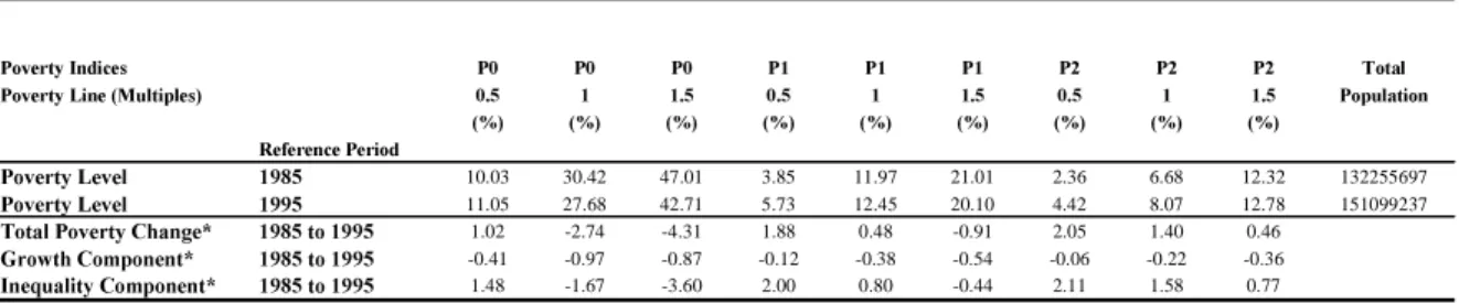
We start analyzing poverty at a National level using PNAD data. We constructed three poverty indices used (P0, P1 and P2). Each of these three poverty indices were calculated according to three poverty lines corresponding to 0.5, 1 and 1.5 of the values of the basic poverty line used adjusted for cost of living differences between Brazilian regions using Rocha´s (1993) estimates. The analysis of these 9 poverty measures performed will be centered on the proportion of poor according to the basic poverty line (i.e., the second column of Table 1). According to Table 1 in 1995 the head-count ratio was 27.7% which combined with the population of 151 million implied in the existence of 41.8 million individuals living below the poverty line.
7DEOH
3RYHUW\&KDQJHV
Table 1 also presents the percentile differences between the 1985 and 1995 poverty profiles adjusted for a rather small rate of per capita GDP growth of 2.09% observed during the period: it shows that using the basic poverty line the proportion of poor fell by 2.74 percentage points which is equivalent to 9% in relative terms. Given the observed shift in income distribution occurred in the period, when higher weights are given to societies poorest segment poverty indices actually rise in the last decade. For the basic poverty line, the poverty gap (P1)
3RYHUW\LQ%UD]LO/HYHODQG&KDQJHV
3RYHUW\,QGLFHV 3 3 3 3 3 3 3 3 3 7RWDO
3RYHUW\/LQH0XOWLSOHV 3RSXODWLRQ
5HIHUHQFH3HULRG
3RYHUW\/HYHO 10.03 30.42 47.01 3.85 11.97 21.01 2.36 6.68 12.32 132255697
3RYHUW\/HYHO 11.05 27.68 42.71 5.73 12.45 20.10 4.42 8.07 12.78 151099237
7RWDO3RYHUW\&KDQJH WR 1.02 -2.74 -4.31 1.88 0.48 -0.91 2.05 1.40 0.46
*URZWK&RPSRQHQW WR -0.41 -0.97 -0.87 -0.12 -0.38 -0.54 -0.06 -0.22 -0.36
,QHTXDOLW\&RPSRQHQW WR 1.48 -1.67 -3.60 2.00 0.80 -0.44 2.11 1.58 0.77
0$5.(76$1'329(57<,1%5$=,/
rose 0.48% percentage points while the average squared poverty gap (P2) rose 1.4 percentage points.
Similarly, all poverty indices present either greater falls or smaller increases when higher poverty lines are used. For the low poverty line the head-count ratio rose 1.02 percentage points and fell 4.31 percentage points when the highest poverty line were used. This respective statistics are 1.88 and -0.91 for the average poverty gap (P1) and 2.05 and 0.46 for the average squared poverty gap (P2). These results altogether implied that the pattern of unbalanced growth across different segments of the Brazilian economy generated different results depending on the binomial poverty measure-poverty line used. This lack of robustness of poverty changes is also influenced by the low per capita GDP growth rate observed in the period (average 0.2% per year).
3RYHUW\&KDQJHV'HFRPSRVLWLRQ
We apply now Datt and Ravallion (1992) decomposition of poverty changes for the 1985-95 period. This decomposition throws light in what is driving the poverty change process discussed above.
The idea is that poverty changes can be better understood in terms of three close determinants: changes in mean per capita income, changes in the degree of inequality of per capita income and changes in a residual term that captures the interaction between these two terms (not presented here). This simple decomposition between a balanced growth component that affects all agents and a redistributive component allows quite general comparisons of poverty changes across different societies and time periods.
The growth-inequality decomposition when applied to the 1985 and 1995 PNADS reveals that growth explains a small part of the changes of the different poverty measures calculated (Table 1). For the head-count ratio, using the basic poverty line, the growth component explains less than one percentile point fall of poverty. The inequality component of poverty change responds to twice the effect of growth for our basic poverty measure. Nevertheless, this is not a robust result. The poverty alleviation effect of the inequality component tends to increase poverty the lower is the poverty line used and the more weight is attributed to the very poor (i.e., P1 and specially P2).
3RYHUW\3URILOH
level. Table 2 presents the three FGT poverty indexes for the basic poverty line proposed. Once again, the analysis will be centered around the head-count ratio for the basic poverty line used.
The overall proportion of poor (P0) during 1995 was 27.7%. As expected, the groups with higher head-counts ratios were headed by: females (33%), young families (15 to 25 years old - 43%), illiterate (43%), non-whites (indigenous (53%) and black (38%)), inhabitants of rural areas (34%), inhabitants of the Northern part of Brazil (North (44%) and North-east region (43%)), working in agriculture (40%) and construction (27%), unemployed (74%) and informal employees (40%).
0$5.(76$1'329(57<,1%5$=,/
7DEOH
$66(76',675,%87,21
The assessment of resources possession will be structured under three headings: 'HFRPSRVLWLRQRI3RYHUW\,QGLFHVDFFRUGLQJWR&KDUDFWHULVWLFVRIWKH+RXVHKROGV
6DPSOH$OO+RXVHKROGV
+HDGRIWKH 7RWDO &RQWULEXWLRQWR7RWDO3RYHUW\
+RXVHKROG 3 3 3 3RSXODWLRQ 3 3 3
7RWDO 27.68 12.45 8.07 100 - -
-*HQGHU
0DOH 26.53 11.40 7.09 82.79 79.35 75.84 72.69
)HPDOH 33.22 17.47 12.81 17.21 20.65 24.16 27.32
$JH
/HVVWKDQ\HDUV 36.99 31.40 29.63 0.02 0.03 0.06 0.09
WR\HDUV 42.95 24.71 19.49 5.73 8.89 11.38 13.84
WR\HDUV 31.71 14.49 9.38 51.24 58.70 59.66 59.55
WR\HDUV 23.88 10.02 6.08 27.87 24.04 22.43 21.00
PRUHWKDQ\HDUV 15.25 5.32 2.95 15.13 8.33 6.47 5.53
<HDUVRI6FKRROLQJ
\HDUV 43.06 19.18 11.84 21.04 32.74 32.43 30.86
WR\HDUV 36.16 16.19 10.20 21.56 28.17 28.05 27.25
WR\HDUV 25.09 10.96 7.23 31.13 28.21 27.40 27.88
WR\HDUV 14.10 6.71 4.86 19.51 9.94 10.52 11.75
PRUHWKDQ\HDUV 3.85 2.94 2.72 6.76 0.94 1.60 2.27
5DFH
,QGLJHQRXV 53.17 27.64 18.23 0.11 0.22 0.25 0.26
:KLWH 18.07 7.89 5.26 53.03 34.62 33.63 34.58
%ODFN 38.82 17.68 11.29 46.31 64.94 65.80 64.76
<HOORZ 10.86 7.24 5.99 0.54 0.21 0.31 0.40
6HFWRURI$FWLYLW\
$JULFXOWXUH 39.81 17.99 11.20 24.69 35.51 35.68 34.27
,QGXVWU\ 21.25 7.83 4.26 15.89 12.20 10.00 8.39
&RQVWUXFWLRQ 27.36 9.75 5.17 9.96 9.85 7.81 6.38
3XEOLF6HFWRU 15.80 5.85 3.09 10.18 5.81 4.79 3.90
6HUYLFH 21.38 8.17 4.49 39.28 30.33 25.80 21.86
:RUNLQJ&ODVV
8QHPSOR\HG 74.02 53.43 46.14 3.18 8.50 13.64 18.16
,QDFWLYH 28.42 15.45 11.90 17.17 17.64 21.32 25.32
(PSOR\HHVZFDUG 19.74 6.36 3.11 27.16 19.37 13.87 10.46
(PSOR\HHVQRFDUG 40.09 15.57 8.30 15.43 22.35 19.30 15.87
6HOI(PSOR\HG 30.75 13.40 8.05 31.12 34.57 33.50 31.02
(PSOR\HU 5.37 2.73 2.03 5.95 1.15 1.30 1.49
3XEOLF6HUYDQW 15.44 5.81 3.10 10.04 5.60 4.68 3.86
8QSDLG 38.20 25.61 21.60 2.27 3.13 4.66 6.07
3RSXODWLRQ'HQVLW\
5XUDO 33.70 15.61 10.23 21.10 25.70 26.47 26.74
8UEDQ 25.36 11.36 7.26 49.25 45.12 44.94 44.32
0HWURSROLWDQ 27.24 12.00 7.88 29.65 29.18 28.59 28.94
5HJLRQ
1RUWK 44.23 20.67 12.96 4.47 7.14 7.42 7.18
1RUWK(DVW 43.12 20.32 13.01 29.56 46.06 48.26 47.66
6RXWK(DVW 20.94 8.94 5.87 43.39 32.82 31.18 31.53
6RXWK 13.49 5.80 3.92 15.16 7.39 7.07 7.37
&HQWHU:HVW 24.61 10.19 6.82 7.41 6.59 6.07 6.27
• Physical capital (financial assets, durable goods, housing, land, public services and transportation)
• Human capital (schooling, technical education, age, experience and learn by doing)
• Social capital (employment, trade unions and associations membership, political participation and family structure).
The availability of new sources of data opens previously unmatched conditions in the Brazilian case to trace an asset profile of the poor. The conjunction of different household surveys opens the possibility of taking a broad picture of assets possession during 1996. Our strategy is to compare the access to different assets in the poor population with the non-poor population.
3K\VLFDOFDSLWDO
The literature on the access of the poor to different types of physical capital is nearly absent in Brazil. We will attempt here to assess the relationship between per capita income and access rates to public services, durable goods and housing.
7DEOH$
$VVHW3RVVHVVLRQ3URILOH3RRU$QG1RQ3RRU3RSXODWLRQ
Access to Housing 3RRU 1RQ3RRU
$FFHVVWR5HQWHGRU&HGHG+RXVLQJ 21.72 0.01% 23.74 0.01%
$FFHVVWR5HQWHG+RXVLQJ 9.91 0.01% 17.21 0.01%
$FHVVWRRZQ+RXVH$OUHDG\3DLG 71.07 0.02% 67.71 0.01%
$FFHVVWR2ZQ+RXVH6WLOO3DLG 5.23 0.01% 7.79 0.00%
Housing Quality 3RRU 1RQ3RRU
$FFHVVWR&RQVWUXFWLRQ 95.62 0.01% 99.19 0.00%
$FFHVVWR%DWKURRP 92.14 0.01% 97.98 0.00%
1RPEHURI,QGLYLGXDOVLQ'ZHOOLQJ 4.05 0.01% 3.03 0.00%
'HQVLW\'RUPLWRU\ 0.58 0.00% 0.37 0.00%
'HQVLW\'ZHOOLQJ 1.43 0.00% 1.04 0.00%
Access to Durables Goods 3RRU 1RQ3RRU
6WRYH 99.65 0.00% 99.91 0.00%
)LOWHU 57.42 0.02% 71.44 0.01%
5HIULJHUDWRU 84.97 0.01% 97.56 0.00%
7HOHSKRQH 13.04 0.01% 39.08 0.01%
5DGLR 92.80 0.01% 97.71 0.00%
&RORU79 72.88 0.02% 93.96 0.00%
79 92.17 0.01% 98.19 0.00%
)UHH]HU 9.12 0.01% 26.93 0.01%
:DVKLQJ0DFKLQH 22.71 0.01% 56.69 0.01%
Access to Public Services 3RRU 1RQ3RRU
:DWHU 90.24 0.01% 97.76 0.00%
6HZDJH 73.65 0.02% 89.33 0.01%
(OHFWULFLW\ 99.49 0.00% 99.89 0.00%
*DUEDJH 80.20 0.01% 94.12 0.00%
- Commuting Time (in minutes) 3RRU 1RQ3RRU
+HDGV$YJ7LPH 38.60 0.02% 42.07 0.01% 6SRXVHV$YJ7LPH 35.89 0.02% 32.79 0.01% +HDGV0RUH7KDQ0LQ 50.70 0.02% 50.95 0.01% 6SRXVHV0RUH7KDQ0LQ 41.13 0.02% 38.79 0.01%
Human Capital 3RRU 1RQ3RRU
$YJ<HDUVRI6FKRROLQJ+HDG 4.70 0.01% 7.16 0.00%
$YJ<HDUVRI6FKRROLQJ6SRXVH 4.59 0.01% 7.05 0.00%
$JH$YHUDJH+HDG 41.47 0.02% 44.91 0.01%
$JH$YHUDJH6SRXVH 37.87 0.02% 40.52 0.01%
7DEOH%
• +RXVLQJDQGODQG
PNAD 96 indicate that dwellings occupation financing of the income poor population is divided approximately as following: 71% live in already paid own housing, 5% live in still paying own housing, 10% live in rented places and 22% live in ceded housing. The
$VVHW3RVVHVVLRQ3URILOH3RRU$QG1RQ3RRU3RSXODWLRQ
Human Capital
Schooling Strictly Greater than 3RRU 1RQ3RRU
+HDG )DWKHU 36.03 0.23% 42.19 0.22%
0RWKHU 38.10 0.24% 45.50 0.23%
6SRXVH )DWKHU 34.84 0.23% 43.88 0.23%
0RWKHU 37.84 0.24% 46.26 0.23%
Specific Human Capital 3RRU 1RQ3RRU
'LG7HFKQLFDO&RXUVH(TXLYDOHQWWR+LJK6FKRRO 8.26 0.13% 17.23 0.17%
%HOLHYHWKDWWR:RUNLQWKH6DPH2FFXSDWLRQLQWKH1H[W<HDUV
57.61 0.24% 67.29 0.21%
78.45 0.20% 83.44 0.17%
)LQG'LIILFXOWWR$GDSWWR1HZ(TXLSDPHQW
17.12 0.18% 16.59 0.17%
17.13 0.18% 16.70 0.17%
Trade Unions and Non
Communitarian Associations Membership 3RRU 1RQ3RRU
7UDGH8QLRQVDQG$VVRFLDWLRQV0HPEHUVKLS
7RWDO 18.17 0.19% 32.62 0.21%
2FFXSLHG 23.63 0.21% 38.26 0.22%
$WWHQGVDW/HDVWRQH0HHWLQJSHU<HDU 2.85 0.08% 6.51 0.11%
$WWHQGVDW/HDVWIRXU0HHWLQJVSHU<HDU 1.94 0.07% 4.57 0.09%
,V1RWD0HPEHUWRGD\EXWZDVLQWKHODVW\HDUV 14.92 0.17% 16.51 0.17%
Communitarian Associations 3RRU 1RQ3RRU
0HPEHUVKLS 11.61 0.16% 14.64 0.16%
$WWHQGVDW/HDVWRQH0HHWLQJSHU<HDU 9.32 0.14% 11.28 0.14%
RI7KRVHWKDWDUH0HPEHUVDUH1HLJKERUKRRG$VVRFLDWLRQV 39.49 0.24% 25.86 0.20%
5HOLJLRXV$VVRFLDWLRQV 36.62 0.24% 34.10 0.22%
$WKHLVW 5.83 0.11% 6.54 0.11%
Political Activities 3RRU 1RQ3RRU
0HPEHUVRI3ROLWLFDO3DUWLHV 3.33 0.09% 5.55 0.10%
3DUWLFLSDQWVLQ3ROLWLFDO3DUWLHV$FWLYLWLHV 43.54 0.24% 37.20 0.22%
KDV/LQNLQJ:LWK3ROLWLFDO3DUWLHV 19.10 0.19% 24.76 0.20%
'RHVQRW8VHDQ\6RXUFHRI,QIRUPDWLRQWR'HFLGH9RWLQJ 41.46 0.24% 33.37 0.21%
2I7KRVHWKDW8VH6RXUFHRI,QIRUPDWLRQ
7KDW8VH79WR'HFLGH9RWLQJ 61.72 0.24% 66.58 0.21%
.QRZVWKH&RUUHFW1DPHRI3UHVLGHQW 76.59 0.21% 89.61 0.14%
.QRZVWKH&RUUHFW1DPHRI0D\RU*RYHQRUDQG3UHVLGHQW 62.15 0.24% 78.50 0.19%
same statistics for non-poor population are: 68% live in already paid own housing, 8% live in
0$5.(76$1'329(57<,1%5$=,/
still paying own housing, 17% live in rented places and 24% live in ceded housing. The comparison between the poor and the non-poor population indicates that the former live more often in already paid own housing and ceded places than the later group1. These statistics show that the renting or still payment of own housing can be perceived are luxury forms of housing financing.
A complementary line of inquiry compares housing quality in both segments: 95 % of the poor (99% of the non-poor population) have access to construction of solid walls, 92% of the poor (98% of the non-poor population) have access to bathrooms inside their houses, the average density per dormitory is 0.58 among the poor (0.37 in the non-poor population) and the average density of family members per dwelling room is 1.43 among the poor (1.04 in the non-poor population). The difference of these last two statistics can be explained by the fact that the poor have larger families than the non-poor population, 4.1 and 3 members respectively. That is, the density of dormitory and dwellings is approximately proportional to the number of individuals in the house. In other words, the house size in number of rooms or dormitories are approximately similar but the poor have larger households.
• 'XUDEOH*RRGV
According to PNAD 96, in Metropolitan Brazil income poor families access rates to durable goods are the following: a) basic goods: stove (99.6 %), water filter (57%), refrigerator (85%), radio (93%), TV (92%). b) luxury goods: telephone (13%), color TV (73%), freezer (9%) and washing machine (23%). These access rates are, in general, higher when we use the sample of non poor individuals: a) basic goods: stove (99.9%), water filter (71%), refrigerator (98%), radio (98%), TV (98%) and Color TV (94%), c) luxury goods: telephone (39%), freezer (27%) and washing machine (57%).
• 3XEOLFVHUYLFHV
The access to basic public goods and services like water, sewage, electricity, communications, public transportation are straight-forward to measure using standard household surveys. According to PNAD 96, the access to public services is more pronounced among the non-poor population: 98% to canalized water, 89% to sewage, 100% to electricity and 94%, garbage collection. The poor population access rates are: 90% to canalized water, 74% to sewage, 99% to electricity and
1
80% garbage collection. There is monotone increase of all these indexes of access to public services analyzed here as me move from the first to the last tenth of per capita income distribution. The increase from the first to the tenth decile for each of these public services non access rates are: 73% to 99% to canalized water, 73% to 98% for sewage, 99.5% to 100% to electricity and 80% to 99% for garbage collection.
• 7UDQVSRUWDWLRQLQIUDVWUXFWXUH
The question used here to capture the quality of transportation in PNAD is: “how long do you take to go to work?”2. One can use this information to assess the transportation cost evaluated at the individual hourly wage rate. Nevertheless, it is not possible to know the exact combination between public and private transportation infrastructure that has led to that outcome. The differences observed between the poor and the non-poor population are not significant: 50% of poor and non poor heads take less than 30 minutes commuting.
+XPDQFDSLWDO
• &RPSOHWHG\HDUVRIVFKRROLQJ
The relation between completed numbers of schooling and poverty is clear from the evidence presented in the previous sections. The average number of completed years of schooling of the head for the poor and the non-poor population: corresponds to 4.7 and 7.2 years respectively. Similarly, the spouses of poor families present also on average two years less schooling than the spouses in the non-poor population, 4.6 and 7 years respectively. This point is noteworthy since completed years of schooling is probably the best approximation to permanent earnings found in Brazilian household surveys.
• $JHDQGH[SHULHQFH
The common approximation to experience used in household surveys is age. The effects of age on poverty plays a central role in this project. We are basically trying to capture what is the life-cycle pattern (if there is any!) of poverty. According to PNAD-96, the average age of the head and spouse in poor families are 41 and 38 years, respectively. While the same variables in the non-poor population are 45 and 41 years, respectively. This two to three years difference may indicate a slight downward trend of poverty incidence measured by the head-count ratio across the life-cycle. That is, as family heads acquire more experience, or accumulate other sorts of capital, the probability of escaping poverty increases .
2
0$5.(76$1'329(57<,1%5$=,/
6RFLDOFDSLWDO
Social capital can be understood in a broad sense by a variety of types of coordination mechanisms (or institutions) that affect the social and private returns of public and private assets. The complementarily between this type of capital and the other types of capital is essential to the understanding of the concept of social capital. For example, the organization of production factors will be a key determinant of the returns obtained from a given amount of physical and human capital accumulated.
• $VVRFLDWLRQVDQG7UDGH8QLRQ0HPEHUVKLS
A first set of social capital indicators are related to enrollment rates in trade unions and non community associations activities. There is an inverse relation between membership rates in such organizations and poverty (18% for poor heads and 33% for non-poor heads).Consistent with this result is the fact that heads with higher level of formal education have higher probabilities of being a members of those organizations. The analysis of the universe of those that are not members of trade unions or non community associations today but were members in the last five years is much closer (15% for poor heads and 16% for non-poor heads) The rates of effective current participation on these activities is much smaller in both groups only 2.9% of poor heads attend at least one meeting per year The same statistic correspond to 6.5 % in the case of non-poor heads.
The membership rate in community associations are much lower (12% for poor heads and 15% for non-poor heads) and more uniformly distributed along the income distribution than the ones found for trade unions and non community associations mentioned above. Nevertheless, the proportion of individuals that attend to at least one meeting per year is higher for community associations than the other types of relationships with associations analyzed. Note that the discrepancy between poor and non poor heads memberships rates (specially controlled for intensity) is also smaller in the case of community associations.
Analysis of community associations composition revealed a greater importance of neighborhood associations (39% for poor heads and 26% for non-poor heads) and religious associations (37% for poor heads and 34% for non-poor heads) among the poor associates.
• 3ROLWLFDO$FWLYLWLHV
heads). The low affiliation rates can be a result of high requirements to political affiliation in terms of active participation.
Given the low rate of formal affiliation to political parties we will use the less stringent concept of having sympathy for political parties (19% for poor heads and 25% for non-poor heads). The qualitative results yield by the two concepts are similar, including its
0$5.(76$1'329(57<,1%5$=,/
relative constancy along the income distribution. One final set of questions on political literacy shows that 77% of poor heads (90% of non-poor heads) knew the correct name of the Brazilian President (Fernando Henrique Cardoso). When one imposes the more stringent condition that the head knew the name of the president, and respective governor and mayors these statistics fell to 62% and 79%, respectively.
3$57329(57<$1'7+(,1&20(*(1(5$7,1*,03$&72)$66(76
The second part of the paper studies how the accumulation of different types of capital impact income-based poverty outcomes.
7+(,03$&72)$66(762:1(56+,321,1&20(%$6('329(57<
A harder and more fundamental question pursued in this part is the role played by capital accumulation on the income generating potential of the poor. A decisive step in this direction is to study the relationship between the possession of different assets and poverty outcomes. In the previous section, we analyzed access rates to different types of capital among the poor and the total population. Now, we start to study possible impacts on poverty of these assets considered jointly and controling for demographics. This exercise aims helping to direct the type of capital enhancing policies to implement.
We analyze here the impacts of human capital, physical assets and social capital on poverty. Human capital and physical assets effects will be studied together using PNAD/96 at a National level. The study of the effects of the social capital items on poverty will be done separately using the special supplement of PME implemented in 1996.
3K\VLFDO&DSLWDO+XPDQ&DSLWDODQG3RYHUW\
This subsection summarizes the relationship between the probability of being poor with demographic variables, various sorts of physical capital and human capital items. Table 4 presents the basic logistic regression estimated.
logistic regression may throw some light on the existing relation (no causality implied in this case) between the possession of each type of asset and poverty outcomes.
Almost all physical capital parameters estimates in the final model were statistically significant at 95% confidence levels and present expected signs, in the sense that having access to a given asset, in general, implies in lower probabilities of being poor. The exceptions are access to electricity with a negative sign. The higher coefficients are found for luxury durable goods and public services such as urban garbage collection (-0.39), telephone (-0.67) and washing machine (-0.65).
0$5.(76$1'329(57<,1%5$=,/
7DEOH
The relationship between poverty and human capital accumulation is less likely to be affected by simultaneity problems, since the former variable is largely accumulated before individuals entered the labor market. This means that one can interpret the relation between poverty and school attainment in a casual manner3. Heads and spouse years of schooling coefficients were around 0.1 and precisely estimated.
3
For example, families with literate heads and spouses have 56% and 36%, respectively, less chances of being poor when compare with being illiterate.
/2*,67,&02'(/2)329(57<+80$1&$3,7$/$1'3+<6,&$/&$3,7$/ $1$/<6,62)3$5$0(7(5(67,0$7(6
9DULDEOHV 2EVHUYDWLRQV (VWLPDWH W6WDWLVWLF 'HYLDQFH
+($'&2/25 :KLWH -0.4298 ** -14.9756 48142.33
+($'(;3(5,(1&( $JH 0.1055 ** 18.1897 48064.62
+($'(;3(5,(1&( $JH6TXDUH -0.0014 ** -14.0000 48053.14
+($'6&+22/,1* &RPSOHWHG<HDUVRI6FKRROLQJ -0.1046 ** -19.3704 39801.87
63286(6&+22/,1* &RPSOHWHG<HDUVRI6FKRROLQJ -0.0948 ** -17.8868 38234.22
+($')$7+(56&+22/,1* &RPSOHWHG<HDUVRI6FKRROLQJ -0.0269 ** -3.4935 38130.38
63286()$7+(56&+22/,1* &RPSOHWHG<HDUVRI6FKRROLQJ -0.0354 ** -4.5974 38026.76
+($'2&&83,(' <HV -1.4012 ** -32.0641 37283.03
63286(2&&83,(' <HV -0.7315 ** -25.2241 36954.01
+($'0,*5$17 <HV -0.1645 ** -5.6336 36710.34
0(75232/,7$1&25( 0.1660 ** 3.3468 36645.68
/$5*(85%$1 %HWZHHQDQG0HWURSROLWDQ -0.0163 -0.3247 36483.95
0(',8085%$1 %HWZHHQDQG -0.0684 -1.3333 36323.87
60$//85%$1 /HVVWKDQLQKDELWDQWV 0.1033 ** 1.9981 36304.32
585$/ 0.1424 ** 2.6273 35902.12
(/(75,&,7< +DV$FFHVV7R 0.2471 ** 3.5351 35742.54
:$7(56833/< +DV$FFHVV7R -0.2979 ** -6.3518 35347.83
85%$16(:$*( +DV$FFHVV7R -0.2342 ** -6.9086 35125.55
85%$1*$5%$*(&2//(&7,21 +DV$FFHVV7R -0.3916 ** -10.9081 34879.08
7(/(3+21( +DV$FFHVV7R -0.6713 ** -15.0854 34347.90
5()5,*(5$725 +DV$FFHVV7R -0.6343 ** -14.0022 33892.99
:$6+,1*0$&+,1( +DV$FFHVV7R -0.6470 ** -17.3458 33512.85
&2/2579 +DV$FFHVV7R -0.6015 ** -16.7083 33224.13
5$',2 +DV$FFHVV7R -0.1490 ** -2.9681 33214.95
$3$570(17 +DV$FFHVV7R -0.4506 ** -5.3643 33183.20
62/,':$//6 +DV$FFHVV7R -0.0724 * -1.9462 33179.42
Value DF Value/DF
Number of Observations : 38698 ; Log Likelihood : -16680.8932 ; Pearson Chi-Square : 42416.600 39000 1.097
$WFRQILGHQFHOHYHO$WFRQILGHQFHOHYHO 7KH2PLWHG&DWHJRU\LV0HWURSROLWDQ3HULSKHU\
educational background were also included in the model. The coefficient of these variables were between one third to one fourth the coefficients found for hea` ` ds and spouses actual educational attainment. This points out the relative importance of the intergeneration transmission of human capital.
Experience is a type of human capital proxied by age present a poverty reduction effect. Age squared was positive and significant indicating the occurrence of decreasing returns to experience. Finally, dummies for the occupied status of heads and spouses presented a negative sign. These dummies can be interpreted as a measure of the rate of utilization of accumulated human capital. The analysis of the life-cycle profile of mean earnings and occupation rates will be implemented in section 6.1.
0$5.(76$1'329(57<,1%5$=,/
6RFLDO&DSLWDODQG3RYHUW\
This subsection summarizes the relationship between the probability of being poor with various sorts of social capital together with demographic variables and human capital variables similar to those used in the previous subsection. The difference is that the present exercise uses PME 96 supplement as data source to take advantage of the social capital variables included in the questionnaire. We should point out that PME income concept and geographic dimensions are more restricted than the ones present in PNAD data used in the logistic regressions presented before. PME income data includes only labor earning in the six main metropolitan regions. On the other hand, we use here a broader sample that also includes single parents households. The idea here is to assess the influences of the presence of spouses on poverty outcomes. In order not to crowd to much the analysis. we did not use spouses characteristics as explanatory variables. Table 5 presents the logistic model estimated.
All variables were statistically significant and presented the expected sign. We implement an analysis of the likelihood ratio of the two states assumed by each dummy variable use. In other words, instead of analyzing the estimated coefficients we look directly at the impact of the different variables on the chances of being poor. The analysis shows that human capital variables of the head and of their parents present the expected signs. Male headed households present a 20% less chances of being poor than female-headed households. The presence of a spouse in the household reduces poverty probability by 23%. This result indicates the importance of marriage as a basic cell of the social capital tissue (see section 6.2.1.). Dependency ratio and heads race present the expected signs as in the previous sub-section exercise. Working class status of the head turn out to have important effects in reducing the probability of being poor: The universe of employees with card has 73% smaller chances of being poor than its complement. The same statistics for other working classes are: public servant 69%, self-employed 45% and employer 78%.
0$5.(76$1'329(57<,1%5$=,/
The analysis of other variables related to the so-called social capital reveals that trade union membership reduces 37% the chances of being poor while the linking to political parties reduces it by less than 9%. Finally, political literacy questions shows that the knowledge of the president name is associated with a 21% on the chances of being in the poverty state.
3$57'<1$0,&$63(&762)329(57<$1'$66(7+2/',1*6
The last effect of increasing asset holdings is to improve poor individuals ability in dealing with adverse income changes. The role played by the consumption smoothing property of assets depends on how important are these changes and how developed are
/2*,67,&02'(/329(57<$1'62&,$/$1'+80$1&$3,7$/ $1$/,6(2)3$5$0(7(5(67,0$7(6
(VWLPDWH W6WDWLVWLF 'HYLDQFH
+HDG6FKRROLQJ ,OOLWHUDWH 0.6183 ** 14.8273 21228.03
+HDG6FKRROLQJ $ERYH&RPSOHWH<HDUV -0.6881 ** -16.9483 19965.82
+HDG)DWKHU6FKRROLQJ ,OOLWHUDWH 0.1853 ** 2.5314 18312.36
+HDG)DWKHU6FKRROLQJ $ERYH&RPSOHWH<HDUV -0.1223 * -1.8092 19202.28
+HDG0RWKHU6FKRROLQJ $ERYH&RPSOHWH<HDUV -0.1780 ** -3.8034 19037.88
*HQGHU 0DOH -0.2289 ** -3.3612 18454.91
,V7KHUHD6SRXVH,Q7KH)DPLO\" <HV -0.2564 ** -2.6190 18607.01
'HSHQGHQF\5DWLR 8S7R -2.4522 ** -64.5316 22151.23
+HDG5DFH %ODFNRU,QGLJHQRXV 0.8305 ** 13.2035 18289.87
:RUNLQJ&ODVV (PSOR\HHV:&DUG -0.9821 ** -21.0300 19429.58
:RUNLQJ&ODVV 3XEOLF6HUYDQW -1.1663 ** -17.1263 18454.91
:RUNLQJ&ODVV 6HOI(PSOR\HG -0.6066 ** -12.2298 18269.70
:RUNLQJ&ODVV (PSOR\HU -1.7377 ** -33.6112 18948.23
7UDGH8QLRQV0HPEHUVKLS <HV -0.4647 ** -8.5896 21274.56
+DV/LQNLQJ:LWK3ROLWLFDO3DUWLHV <HV -0.1323 ** -3.1727 21228.03
.QRZV7KH&RUUHFW1DPH 2I7KH3UHVLGHQW -0.2341 ** -3.5470 21127.46
.QRZV7KH&RUUHFW1DPH 0D\RU*RYHUQRUDQG3UHV -0.1722 ** -3.1830 21274.56
DF Value Value/DF Number of Observations : 18308 ; Log Likelihood : -10371.4604 ; Pearson Chi-Square : 18000.00 18206.932 0.996
this last effect requires an analysis of dynamic properties of poor individuals income processes and an evaluation of institutions that constraint their financial behavior.
Sections 6 to 8 study interactions between these two segments earning process and asset holdings behavior taking into consideration different time horizons. Long-run issues, studied on section 6, are related to the study of low frequency income fluctuations and the life-cycle profile of assets holdings using cohort analysis. The following two sections assess the poor behavior and/or welfare losses associated with short-run income fluctuations. Section 7 evaluates short-run dynamics of per capita earnings and poverty measures using panel data. Section 8 analyzes poor households financial behavior in dealing with high frequency gaps between income and desired consumption.
7+(/,)(&<&/(
This section studies some effects of low frequency earning dynamics and asset accumulation on the welfare level of the poor.
/RQJUXQ+RXVHKROG3HU&DSLWD(DUQLQJV
The life-cycle behavior of any variable can be studied using a static age profile or more interesting using pseudo-panels. In the static profile, we plot from a cross-section the value assumed by any chosen variable in various age groups. The main limitation of the static age profile is not taking into account cohort or year effects. Instead in the pseudo-panel, we track the value of a certain statistic for the same generation across time. We will use this later approach here.
We start with the life-cycle pattern of per capita earnings levels and dispersion depends on the interaction between heads, spouses and other members of the households number, occupation rates and earnings levels. The Graphs 1 and 2 presents the life-cycle profile of
0$5.(76$1'329(57<,1%5$=,/
$VVHWV3RVVHVVLRQLQD/LIH&\FOH3HUVSHFWLYH
This sub-section describes the dynamics of the possession of selected types of assets across the life-cycle.
6SRXVHV6KDUHLQ)DPLO\(DUQLQJVDQG3RYHUW\
The family can be perceived as the basic cell of the social capital tissue. For instance, the participation of spouses in the labor market can offset some of the effects of the fall of heads earnings at latter stages of the life-cycle. In particular, we want to investigate here whether the life-cycle pattern of spouse earnings share in total family earnings differs in poor and non poor households. We use at this point the median school attainment of households heads as the border line between poor and non poor households4. The high explanatory power of household heads schooling on poverty measures presented in parts 1 and 2 gives support to this procedure.
Graphs 3 and 4 presents the age profile of the share of spouse earnings in total household earnings for poor and non poor families of different generations The upper limits of these curves can be read as the latter year (1997) static age profile of this variable. This static profile reveals that the share of spouse earnings in total household earnings for poor families presents an increase from 15% in the 25-30 age bracket to 20% in the 65-70
0$5.(76$1'329(57<,1%5$=,/
bracket. This same statistic for non poor families does roughly the opposite movement falling from 21% in the 25-30 age bracket to 14% in the 65-70 age bracket.
If we unravel the path of this statistic for each generation across time we find that the sharp increase of spouse earnings in family earnings observed in the last 15 years was not uniform across different cohorts of the Brazilian society.
4 We thank Miguel Székely for this suggestion.
*UDSK *UDSK
+RXVHKROG$YHUDJH3HU&DSLWD(DUQLQJV +RXVHKROG3HU&DSLWD(DUQLQJV'LVSHUVLRQ*,1,
6RXUFH PME 82, 87, 92 and 97 (yearly averages) - Obs: normalized by yearly total averages 0.60
0.80 1.00 1.20 1.40 1.60 1.80
15-20 20-25 25-30 30-35 35-40 40-45 45-50 50-55 55-60 60-65 65-70 0.75 0.80 0.85 0.90 0.95 1.00 1.05 1.10 1.15
Graph 4 shows that the increased participation of spouses in the household budget in non poor families was basically driven by young cohorts sharply (i.e., less than 40-45 years in 1982) that increased while the same statistic for older cohorts stayed roughly constant across time. For example, the spouse share within the generation that was in the 20-25 bracket in 1982 increased from 15% to 23% in 1997 while the same statistic for the generation that was in the 50-55 bracket in 1982 rose only from 12% to 14% during the same period.
In contrast, within the poor segment the sharp increase on the share of spouse earnings on household earnings affected on a roughly uniform way all cohorts. For example, the spouse share of the generation that was in the 20-25 bracket in 1982 increased from 11% to 19% in 1997 while the same statistic for the generation that was in the 50-55 bracket in 1982 rose from 11% to 20% during this period.
3XEOLF6HUYLFHV
We briefly analyze the evolution of two types of physical assets across the life-cycle: public services provision and house ownership.
Non access rates to different public services (water, sewage, electricity and garbage collection), decreased substantially in a roughly homogeneous way across different cohorts during the 1976-96 period. During this period, for example as Graph 5 shows, the no access rates to garbage collection to the generation that
0$5.(76$1'329(57<,1%5$=,/
was in the 45-50 age bracket in 1996 decreased from 31.3 % in 1976 to 10.7% in 1996. The slope of the non access rates lines for different cohorts becomes somewhat less steep in the 1990 to 1996 period. In this sense the 1980s decade can not be labeled as a ‘lost decade’ in terms of the provision of public services.
+RXVLQJ
*UDSK *UDSK
1RQ3RRU 3RRU
6RXUFH PME 82, 87, 92 and 97 (yearly averages)
5 7 9 11 13 15 17 19 21 23 25
20-25 25-30 30-35 35-40 40-45 45-50 50-55 55-60 60-65 65-70 5 7 9 11 13 15 17 19 21
6+257581($51,1*6'<1$0,&6$1'7+(:(/)$5(2)7+(3225
Earnings dynamics is an essential determinant of asset holdings and the level of welfare of those located at the lower tail of income distribution. This section assesses three short-run dynamic inter-connected issues: i) the extension of per capita earnings volatility measured at an individual level. ii) the intensity of movements into and out of earnings based poverty states. iii) the impact of the period used to measure income on aggregate poverty measures.
3RRUDQG1RQ3RRU3HU&DSLWD(DUQLQJV9RODWLOLW\
The Brazilian case offers the possibility of assessing per capita earnings dynamics using longitudinal information found in PME. PME replicates the US Current Population Survey (CPS) sampling scheme attempting to collect information on the same dwelling eight times during a period of 16 months. More specifically, PME attempts to collect information on the same dwelling during months t, t+1, t+2, t+3, t+12, t+13, t+14, t+15.
The first aspect to be analyzed here is the extend of per capita short run volatility in the poor and non-poor Brazilian segments. Besides mean earnings levels and dispersion, the earnings volatility constitute a key determinant of the level of social welfare. The longitudinal information used in this analysis were obtained by concatenating observations of the same individuals during four consecutive
*UDSK *UDSK
1R$FHVVWR*DUEDJH&ROOHFWLRQ 'R1RW2ZQ+RXVH$OUHDG\3DLG
0$5.(76$1'329(57<,1%5$=,/
observations5 then we calculated the average temporal variance of individual log per capita earnings across four consecutive months. The inspection of these time
series of temporal variability of earnings indicate the presence of bumps in the series that coincided with inflation peaks that were followed by stabilization plans in 1986, 1990 and 1994. These bumps indicate the influence exerted by the observed inflationary instability on per capita income volatility.
The average temporal variance of log per capita earnings corresponds to 0.158 in the 1983-96 period. This statistic is more noisy than the corresponding ones found for the non-poor population (0.124). Furthermore, this is a robust result across time since it holds for all 182 months this statistic was calculated. A similar exercise was done using the median heads education as the criteria to separate the poor from the non poor. Human capital poor families presented a variability of per capita earnings equal to 0.139 of while the corresponding statistic for rest of the population was slightly higher 0.143.
3RYHUW\'\QDPLFV
A high degree of social mobility is normally viewed as a good attribute of a given society. However, depending on how social mobility is defined and measured, one can end up labeling part of the existing income instability as social mobility6. For one thing, if we are measuring a strictly positive economic variable such as consumption, higher variance translated as risk, could be perceived as a quality. In the sense that when one can only get better, higher variability enhances his/her chances of going out of the bad state. This subsection presents unidirectional measures of per capita earnings mobility. In particular, we estimate the transition probabilities into and out of poverty7 according to different horizons. Estimates of these transition probabilities for the 1996-98 period are presented in Table 6.
5
In the case of individuals successfully observed during eight times, each block of four consecutive observations were treated separately.
6
The distinction between circular and structural mobility is key here.
7 Formally, t = P[Y2<L\Y1>L] and s = P[Y2>L\Y1<L] where Yi is income in period i and L is the poverty line used. Assuming the
environment is time-homogeneous and we have reached steady-state, these transition probabilities, t and s, measures the proportion of non-poor households becoming poor each month and the proportion of poor households escaping poverty each month, respectively. If we assume the process is Markovian, then these transition probabilities still have this interpretation even if we have not reached yet the steady-state.
7DEOH
6DPSOH 7RWDO /RZ +LJK
3RSXODWLRQ 6FKRROLQJ 6FKRROLQJ
3HULRG 0RYHPHQW ,1 287 ,1 287 ,1 287
PRQWKV E\ 9.77% 24.84% 13.24% 21.51% 6.30% 28.18%
PRQWKV E\ 8.95% 27.00% 12.48% 23.60% 5.42% 30.40%
PRQWK E\ 8.21% 25.23% 9.64% 22.56% 6.77% 27.90%
They reveal that for the basic poverty line used: i) when we compare poverty measured at a 4-month period one year apart 9.77% and 24.84%. ii) when we compare two isolated months one year apart these probabilities are 8.95% and 27%. iii) on a month by month basis the entering and exiting probabilities correspond to 8.21% and 25.23%.The magnitude of these transition probabilities reveals a degree of mobility in and out of poverty which seems to be above expected.
When we split the sample between poor and non poor according to heads median school level we observe, as expected, higher entering probabilities and lower exiting probabilities for human capital poor families. For example, the probability of entering poverty between 12-months based on 4-month period earnings corresponds to 13.24% for poor against 6.3% for the non-poor population. The corresponding poverty exiting probabilities are 21.51%for the education poor and 28.18% for the remaining population.
7HPSRUDODJJUHJDWLRQ
Our final exercise is to compare different poverty measures using two different windows to measure earnings: 1-month and 4-month periods. To be sure, we compare poverty measures for a period of 4 consecutive months obtained using average per capita income during this 4-month period and the results obtained treating each observation independently. Table 7 presents yearly averages of FGT poverty indexes (P0, P1 and P2) during the 1985-96 period.
The difference between the poverty measures using the 4-month and the 1-month period is striking, specially as we move to measures that take into consideration inequality among the poor. During the whole period the differences amounted to 11% for P0, 24% for P1 and 32% for P2. In certain periods of high economic instability, like 1989, the difference of the Squared Poverty Gap (P2) reaches an annual average of more than 40%8.
To evaluate the suitability of different windows of income measurement implicit in poverty measures, one needs to make explicit hypothesis about the functioning of capital markets. The reason is that individuals extract utility from consumption and not from labor income itself. The operation of capital markets allows to smooth consumption in spite of earnings fluctuations. In a complete markets setting the relevant concept of income would correspond to the permanent income over the planning horizon of the individual. On the other hand, the existence of capital market failures would imply the imposition of restrictions on period used to measure earnings. In other words, capital
8
market failures truncates the horizon that agents can implement their decisions. In this case it makes sense using shorter periods of poverty measurement.
0$5.(76$1'329(57<,1%5$=,/
7DEOH
3RYHUW\0HDVXUHV<HDUO\$YHUDJHV
6+257581),1$1&,$/%(+$9,252)7+(3225
This section aims to discuss the effects of the short-run earnings dynamics discussed along the previous section on poor household units financial behavior and welfare.
We start tracing a profile of poor savers according to ABECIP surveys. ABECIP surveys on consumers finances during 1987, shows that 47% of adults did not possess any financial asset. This statistic raises to 70% in the poor segment of the population. These surveys also reveal that the most popular financial asset in Brazil are Savings GHSRVLWV FDGHUQHWDVGHSRXSDQoD). 95% of poor individuals that held any asset, held only savings deposits. This means that little is loss when one restrict the analysis of the poor financial holdings to savings deposits. In 1987, there were 70 millions active savings accounts in Brazil. Of course, each individual can hold more than one account. However, Abecip data shows that the average number of accounts per user of savings deposits was 1.42.
A first explanation for the popularity of savings deposits is the low level of requirements imposed on individuals to open savings deposits. This level of requirements are explained by the operational simplicity granted by the monthly capitalization period of savings accounts. The philosophy adopted when savings deposits were first introduced implied in the absence of entry barriers in official institutions, like Caixa Econômica Federal. In 1987, 36% of owners of savings accounts had deposits in this institution.
3RYHUW\,QGH[ 3 3 3
7LPH3HULRG 0217+ 0217+; 0217+ 0217+; 0217+ 0217+;
0.23661 0.26116 0.11577 0.14564 0.08113 0.11261
0.15484 0.18218 0.07600 0.10536 0.05448 0.08494
0.15918 0.18941 0.07648 0.10621 0.05443 0.08403
0.16677 0.19694 0.07845 0.10980 0.05509 0.08724
0.15907 0.19528 0.07492 0.11176 0.05336 0.09004
0.18763 0.22240 0.08699 0.12264 0.05977 0.09502
0.23720 0.26579 0.11157 0.14434 0.07597 0.10982
0.31018 0.33694 0.15155 0.18682 0.10356 0.14154
0.30660 0.33632 0.15418 0.19305 0.10845 0.15086
0.32546 0.35277 0.16398 0.20348 0.11413 0.15775
0.25592 0.28541 0.12674 0.16394 0.08921 0.12878
0.22835 0.25284 0.11398 0.14860 0.08098 0.11886
SRVVHVVLRQRIVDYLQJVDFFRXQWV where the items RSHQLQJOLPLWZD\WRRKLJK appears with a null proportion even in the poorest segments of the population. On the other hand, the difficult access to other assets besides savings deposits is captured by the fact that no poor adult justified forQRSRVVHVVLRQRIVDYLQJVDFFRXQWVbecause he or she SUHIHUVWRXVH DQRWKHUDVVHWAt the same time 37% of the high income group presented thisjustification forQRSRVVHVVLRQRIVDYLQJVDFFRXQWV.
0$5.(76$1'329(57<,1%5$=,/
As expected, average balances of savings deposits of the poorest individuals were inferior to those of higher income brackets, 5.1 minimum wages against 21.8 minimum wages. However, the ratio between average balances to income was higher in group of poor owners of savings accounts, 2.5 against 1.1. If we compute as well the zero balances of individuals that did not hold savings deposits, the ratio between average balances to income of these two income groups become more similar, 0.72 and 0.64, respectively. This result may be attributable to the higher portfolio diversification of higher income groups. At the same time it reinforces the importance of savings deposits among the poorest segments of Brazilian population.
The automatic determination of savings deposits nominal interest rates as 0.5% per month plus lagged monetary correction implied that transitions towards higher inflation rates generated real interest rates losses. Similarly, transitions towards lower monthly inflation rates were followed by rises in savings deposits real interest rates. For example, the inflation rise observed after the failure of the Cruzado plan in 1986 (from 3% per month to 20% per month in one year ) implied in an erosion of 14% on the real value of savings deposits. This lagged monetary correction mechanism was not always understood by economic actors. According to 1985 Abecip survey, 18% of individuals with unfinished primary school agreed with the proposition that VDYLQJV GHSRVLWV QRPLQDO LQWHUHVW UDWHV DOZD\V VXUSDVVHV WKH LQIODWLRQ UDWH. On the other extreme, only 3% of individuals with a university degree would agree with this proposition9.
Among the characteristics recognized as important by deposit holders, risk ,captured by items such as VHFXULW\or ZDUUDQWHGE\WKHJRYHUQPHQW, appears in first place among the poorest segments and the richest segments of the population. In second place papers the attribute, H[SHFWHG UHWXUQ, 26% and 40% respectively. /LTXLGLW\appears in third place, 5% and 6%, respectively. Besides the trinity return, risk and liquidity the item HDV\WRXVH presented 4% and 3% of answers, respectively.
The poorest segments appear to attribute a higher value to risk. On the other hand, expected return appears to be more important among the richest groups, reflecting the higher margin of substitution between assets observed. The low importance attributed to liquidity is explained by the monthly capitalization period of savings deposits. This low liquidity imposed difficulties in the use of savings deposits as a flight from money mechanism in the interval between wage payments.
9
An anedotic evidence of the difficulty faced by the poor to deal with inflationary complexities is that the only asset which the poor
presented higher access rates were bonus from %D~ GD )HOLFLGDGH These assets were well known for not offering any type of
Most of operations with savings deposits presented a high frequency. The average date of the last deposit was 6.9 months for the poorest segment and 3.7 months for the higher income bracket. On the other hand, the average date of the last withdrawal was 4.9 months and 5.2 months, respectively.
The main reasons presented IRU LQWHQGLQJ QRW WR GHSRVLW LQ VDYLQJV GHSRVLWV LQ WKH QH[W IHZPRQWKV were the fact that there was no remaining money or MXVWOLWWOHPRQH\OHIW (90% for the poorest segment and 46% for the richest segments). On the other hand, the main
0$5.(76$1'329(57<,1%5$=,/
motivation presented IRULQWHQGLQJWRZLWKGUDZPRQH\IURPVDYLQJVGHSRVLWVLQWKHQH[W IHZPRQWKVwas WRFRPSOHPHQWGRPHVWLFEXGJHW (83% for the poorest segment and 36% for the richest segment). These justifications combined with the high frequencies of savings deposits and withdraws suggest a consumption smoothing process with respect to short run fluctuations of family income.
The consumption smoothing process appears to be more intense among the poorest savings deposits holders. This result is consistent with evidences of a high variability of family income in the lower tail of the distribution mentioned in section 7. The high frequency and the low duration of poverty spells can be explained by unemployment spells with similar characteristics, like those frequently reported for Brazilian labor markets. Although, the item ,DPXQHPSOR\HG explain little of ex-post savings deposits withdrawals, the unemployment motivation can be implicit in more general justifications presented. The most important justifications presented WRKDYHZLWKGUDZDOIURPVDYLQJV GHSRVLWVwere: WRFRPSOHPHQWGRPHVWLFEXGJHW(56% for the poorest segment and 26% for the richest segment) and for an emergency (21% for the poorest segment and 22% for the richest segment).
&21&/86,216
This paper attempted to establish a basis of research on the relationship between poverty, resources distribution and asset markets operation in Brazil. The final target is to guide the implementation of different capital enhancing policies.
The availability of new sources of data opened previously unmatched conditions in Brazilian metropolitan areas to implement an analysis of asset possession and poverty. The assessment of resources distribution was structured under three headings: Physical capital, Human capital and Social capital.
The paper provided a threefold map of the different effects that the possession of these different assets may have on poverty. Accordingly, the paper was divided in three parts: the first part considered the direct welfare effect derived from owning higher asset levels. The second part assessed the impact of owning higher asset levels on the income generating potential of the poor. The third, and most important part of the paper, discussed the effects of higher asset holdings on the poor ability to smooth adverse income changes.
• 0DLQ5HVXOWV
In 1995, the Brazilian head-count ratio was 27.7% which implied the existence of 41.8 million individuals living below the poverty line. In 1985, this statistic reached 30.4%. Since there was meager growth between these two years, most of the change in P0 observed can be attributed to a reduction in inequality levels. Nevertheless, this qualitative result is not a robust to changes in poverty measures and poverty lines used. Standard poverty profiles showed that, as expected, completed years of schooling appears to be the most important among all socio-economic variables used to explain poverty.
Similarly, private assets can be divided in terms of these two categories: water filter, color TV, freezer and washing machine presented a luxury goods profile. While stove, refrigerator, radio, TV, radio and housing ownership were more uniformly distributed along the income distribution. The analysis pointed out the need to consider qualitative aspects especially for housing and transportation items.
Access rates to different items of the social capital portfolio considered presented a richer pattern when one compares the poor and the non poor population. Membership in professional associations (i.e., trade-unions, cooperatives) is much higher among the non
0$5.(76$1'329(57<,1%5$=,/
poor while membership in community associations (i.e., neighborhood and religious) was more uniformly distributed. Finally, formal affiliation rates to political parties were found to be differentiated poor and non poor segments but were found to be small.
The second part of the paper applied logistic regressions to study the income generating effects of the assets portfolio mentioned above on income-based poverty measures. The approach differs from the one implemented in the first section for two basic reasons. First, we considered the effect of the assets jointly and also taking into account demographic and regional variables. Second, we attempted to give a more casual interpretation to the results found, as the potential role of the provision of different assets to fight poverty. This interpretation is only warranted for human capital variables and demographics. Nevertheless, we believe that this logistic regression may throw light on the existing partial relation (no causality implied in this case) between the possession of each type of asset and poverty outcomes.
The results found were consistent, qualitatively speaking, to the ones found in the first part of the paper. It is worth emphasizing the role played by heads and spouses completed years of schooling variables, as well as the family background variables to explain poverty. This result provided us confidence to use head of household median years of schooling as a classification variable to split the sample in poor and non poor households. In other words, years of education was used as a proxy for per capita permanent earnings in the analysis of income dynamics performed in the last part of the paper.
The third part of the paper studied dynamic properties of the relationship between poverty and asset holdings. The basic unit of capital accumulation/allocation decisions considered here is the household. There will be two basic time horizons to be looked here: the life-cycle (with cohort data) and up to 16-month intervals (with panel data).
issues. In terms of short-run earnings dynamics, we used short panels and the main results found were: i) earnings volatility - The average temporal variance of log per capita earnings corresponds to 0.158 in the 1983-96 period. This statistic is more noisy than the corresponding ones found for the non-poor population (0.124). ii) poverty dynamics - the probability of entering poverty between 12-months based on 4-month period earnings corresponds to 13.24% for the education poor against 6.3% for the remaining population. iii) Poverty and temporal aggregation - The difference between aggregate poverty measures using the 4-month and the 1-month period is striking, specially as we move to measures that take into consideration inequality among the poor. The estimated average differences amounted to 11% for P0, 24% for P1 and 32% for P2.
0$5.(76$1'329(57<,1%5$=,/
$11(;(
The life-cycle behavior of any variable can be studied using a static age profile or more interesting using pseudo-panels. In the static profile, we plot from a cross-section the value assumed by any chosen variable in various age groups. The main limitation of the static age profile is not taking into account cohort or year effects. Instead in the pseudo-panel, we track the value of a certain statistic for the same generation across time. We will use both approaches here to study the long run accumulation of various types of capital in Brasil during the last 20 years.
%5$6,/0(75232/,7$1 ($51,1*6 6RXUFH31$',%*( 5DWLRRI+HDGODERU(DUQLQJVWR+RXVHKROGODERU(DUQLQJV 20 30 40 50 60 70 80 90 100 15-20 20-25 25-30 30-35 35-40 40-45 45-50 50-55 55-60 60-65 65-70 10 20 30 40 50 60 70 80 90 100
15-20 20-25 25-30 30-35 35-40 40-45 45-50 50-55 55-60 60-65 65-70 >70 76 81 85 90 93 96
5DWLRRI6SRXVHODERU(DUQLQJVWR+RXVHKROGODERU(DUQLQJV 2 7 12 17 22 27 15-20 20-25 25-30 30-35 35-40 40-45 45-50 50-55 55-60 60-65 65-70 2 7 12 17 22 27
15-20 20-25 25-30 30-35 35-40 40-45 45-50 50-55 55-60 60-65 65-70 >70
6RXUFH31$',%*( 6&+22/,1*%5$6,/0(75232/,7$1 6RXUFH31$',%*( 50 55 60 65 70 75 80 85 90 95 15-20 20-25 25-30 30-35 35-40 40-45 45-50 50-55 55-60 60-65 65-70 50 55 60 65 70 75 80 85 90 95 15-20 20-25 25-30 30-35 35-40 40-45 45-50 50-55 55-60 60-65 65-70 >70
76 81 85 90 93 96
5DWLRRI6SRXVHDOO6RXUFHV(DUQLQJVWR+RXVHKROGDOO6RXUFHV(DUQLQJV 2 7 12 17 22 27 32 37 15-20 20-25 25-30 30-35 35-40 40-45 45-50 50-55 55-60 60-65 65-70 2 7 12 17 22 27 32 37 15-20 20-25 25-30 30-35 35-40 40-45 45-50 50-55 55-60 60-65 65-70 >70
76 81 85 90 93 96
$YHUDJH<HDUVRI6FKRROLQJ 3.00 3.50 4.00 4.50 5.00 5.50 6.00 6.50 7.00 7.50 8.00 15-20 20-25 25-30 30-35 35-40 40-45 45-50 50-55 55-60 60-65 65-70 3.0 3.5 4.0 4.5 5.0 5.5 6.0 6.5 7.0 7.5 8.0
15-20 20-25 25-30 30-35 35-40 40-45 45-50 50-55 55-60 60-65 65-70 >70
76 81 85 90 93 96
$YHUDJH<HDUVRI6FKRROLQJ+HDG 3.0 3.5 4.0 4.5 5.0 5.5 6.0 6.5 7.0 7.5 8.0 15-20 20-25 25-30 30-35 35-40 40-45 45-50 50-55 55-60 60-65 65-70 3.0 3.5 4.0 4.5 5.0 5.5 6.0 6.5 7.0 7.5 8.0
15-20 20-25 25-30 30-35 35-40 40-45 45-50 50-55 55-60 60-65 65-70 >70
$66(73266(7,21+RXVLQJ4XDOLW\ 6RXUFH31$',%*( $66(73266(7,21$FFHVVWR+RXVLQJ 6RXUFH31$',%*( 1R$FFHVVWR%DWKURRP 0 5 10 15 20 25 30 35 40
15-20 20-25 25-30 30-35 35-40 40-45 45-50 50-55 55-60 60-65 65-70 0 5 10 15 20 25 30 35 40
15-20 20-25 25-30 30-35 35-40 40-45 45-50 50-55 55-60 60-65 65-70 >70
81 85 90 93 96
$FFHVVWR5HQWHGRU&HGHG+RXVLQJ 5 15 25 35 45 55 65 75 85
15-20 20-25 25-30 30-35 35-40 40-45 45-50 50-55 55-60 60-65 65-70 5 15 25 35 45 55 65 75 85
15-20 20-25 25-30 30-35 35-40 40-45 45-50 50-55 55-60 60-65 65-70 >70
76 81 85 90 93 96
$FFHVVWR5HQWHG+RXVLQJ 5 15 25 35 45 55 65
15-20 20-25 25-30 30-35 35-40 40-45 45-50 50-55 55-60 60-65 65-70 5 15 25 35 45 55 65
15-20 20-25 25-30 30-35 35-40 40-45 45-50 50-55 55-60 60-65 65-70 >70
76 81 85 90 93 96
1R$FFHVVWR&RQVWUXFWLRQ 0.00 1.00 2.00 3.00 4.00 5.00 6.00 20-25 25-30 30-35 35-40 40-45 45-50 50-55 55-60 60-65 65-70 0.00 1.00 2.00 3.00 4.00 5.00 6.00
20-25 25-30 30-35 35-40 40-45 45-50 50-55 55-60 60-65 65-70 >70
Source : PNAD/IBGE
1R$FFHVVWRRZQ+RXVH$OUHDG\3DLG
10 20 30 40 50 60 70 80 90
15-20 20-25 25-30 30-35 35-40 40-45 45-50 50-55 55-60 60-65 65-70 10 20 30 40 50 60 70 80 90
15-20 20-25 25-30 30-35 35-40 40-45 45-50 50-55 55-60 60-65 65-70 >70
76 81 85 90 93 96
75 80 85 90 95 100
15-20 20-25 25-30 30-35 35-40 40-45 45-50 50-55 55-60 60-65 65-70 75 80 85 90 95 100
15-20 20-25 25-30 30-35 35-40 40-45 45-50 50-55 55-60 60-65 65-70 >70
$66(73266(7,21±1R$FFHVVWR'XUDEOHV*RRGV 6RXUFH31$',%*( )LOWHU 10 20 30 40 50 60 70 80 15-20 20-25 25-30 30-35 35-40 40-45 45-50 50-55 55-60 60-65 65-70 10 20 30 40 50 60 70 80
15-20 20-25 25-30 30-35 35-40 40-45 45-50 50-55 55-60 60-65 65-70 >70
81 85 90 93 96
5HIULJHUDWRU 0 10 20 30 40 50 60 70 80 15-20 20-25 25-30 30-35 35-40 40-45 45-50 50-55 55-60 60-65 65-70 0 10 20 30 40 50 60 70 80
15-20 20-25 25-30 30-35 35-40 40-45 45-50 50-55 55-60 60-65 65-70 >70
76 81 85 90 93 96
6WRYH 0.00 0.50 1.00 1.50 2.00 2.50 3.00 3.50 4.00 20-25 25-30 30-35 35-40 40-45 45-50 50-55 55-60 60-65 65-70 >7 0 0.00 0.50 1.00 1.50 2.00 2.50 3.00 3.50 4.00
20-25 25-30 30-35 35-40 40-45 45-50 50-55 55-60 60-65 65-70 >70
76 81 85 90 93 96
*DUEDJH&ROOHFWLRQ 5 10 15 20 25 30 35 40 15-20 20-25 25-30 30-35 35-40 40-45 45-50 50-55 55-60 60-65 65-70 5 10 15 20 25 30 35 40
15-20 20-25 25-30 30-35 35-40 40-45 45-50 50-55 55-60 60-65 65-70 >70
6RXUFH31$',%*( :DWHU 0 5 10 15 20 25 30 35 40 15-20 20-25 25-30 30-35 35-40 40-45 45-50 50-55 55-60 60-65 65-70 0 5 10 15 20 25 30 35 40
15-20 20-25 25-30 30-35 35-40 40-45 45-50 50-55 55-60 60-65 65-70 >70
81 85 90 93 96
(OHFWULFLW\ 0 2 4 6 8 10 12 14
15-20 20-25 25-30 30-35 35-40 40-45 45-50 50-55 55-60 60-65 65-70 0 2 4 6 8 10 12 14
15-20 20-25 25-30 30-35 35-40 40-45 45-50 50-55 55-60 60-65 65-70 >70
76 81 85 90 93 96
6HZDJH 30 35 40 45 50 55 60 65 70 75 80
15-20 20-25 25-30 30-35 35-40 40-45 45-50 50-55 55-60 60-65 65-70 20 30 40 50 60 70 80 90
15-20 20-25 25-30 30-35 35-40 40-45 45-50 50-55 55-60 60-65 65-70 >70
$66(73266(7,21±(PSOR\PHQW
6RXUFH31$',%*(
1RQ$FFHVVWR2FFXSDWLRQ+HDG
5.00 15.00 25.00 35.00 45.00 55.00 65.00 75.00 85.00 95.00 105.00
15-20 20-25 25-30 30-35 35-40 40-45 45-50 50-55 55-60 60-65 65-70 >70
1982 1987 1992 1997
5.00 15.00 25.00 35.00 45.00 55.00 65.00 75.00 85.00
15-20 20-25 25-30 30-35 35-40 40-45 45-50 50-55 55-60 60-65 65-70
1RQ$FFHVVWR2FFXSDWLRQ6SRXVH
45.00 50.00 55.00 60.00 65.00 70.00 75.00 80.00 85.00 90.00 95.00
15-20 20-25 25-30 30-35 35-40 40-45 45-50 50-55 55-60 60-65 65-70 >70
1982 1987 1992 1997
45.00 50.00 55.00 60.00 65.00 70.00 75.00 80.00 85.00 90.00