The evolution of wage inequality in Brazil, 1976 to 1997

' - . ...,...FUNDAÇÃO ' - . GETULIO VARGAS

SEMIN,\RIOS

DI: PI-

S()U

I

SA

LCONOl\lIC,\

Escola de Pós-Graduação em Economia

"The Evolution or Wage

Inequality in Brazil,

1976

to

1997"

\

Prof. Orlando J. Sotomayor

(University ofPuerto Rico at Mayaguez)

LOCAL

Praia de Botafogo, 190 - 10° andar - Auditório- Eugênio Gudin

DATA

20/07/2000 (5" feira)

HOR.ÁRIO 16:00h

The rising trends in inequality in the distribution of earned income continued

into the decade of the 1970s.15 However, a distinction has to be made between the early

and late 1970s. While inequality increased during the first half of the decade, it did

decline during its second half. 16 In the end, however, the net effect was a rise in

inequality, though not as large as that which occurred during the earlier decade. As to

the causes of the latter part of the decade's decline in wage concentration, Fishlow et. a!.

point to a fali in returns to labor that the authors attribute to an upward trend in the

business cycle.17 The theoretical foundation of their argument is that of the practice of

labor hoarding, which produces higher skill differentials during recessions and lower

differences during periods of gro\\ih.

The decade of the 1980s presented a very different macroeconomic picture than

that ofthe earlier ones. Contrary to the earlier 20-year period where ali groups enjoyed

improvements in mean income levels- albeit significantly greater for the upper income

groups-, the decade of the 1980s produced an increase only at the very top of the

distribution- and even then a modest one. 18 Inequality, as measured by a variety of

indices rose markedly, though again not as strongly as it did during the 1960s. As to the

causes of the changes, Fishlow et. a!. point to a rise in returns to labor, now associated

with a stagnating economy.19 With a longer time period in which to make inferences and

test hypothesis, Bonelli and Ramos conclude that the short term negative relationship

between growth and equality for the upturn period 1976-1980 and the downturn period

1981-83 had become blurred by the latter half of the decade whence inflation heated up

considerably.20 After then grO'Wih carne accompanied by significantly higher inequality.

,

..

negative relationship.21 The study also confirrns the rise in dispersion for the decade of

the 1980s and its acceleration during its latter half.

A common thread among studies is the empirically established importance of

education as a major deterrninant ofwage variation. It then seems natural that such a

state of affairs motivated in-depth studies on the relationship between education and

inequality. Fishlow's and Langoni's seminal decomposition results associating education

with up to fifty percent of all wage dispersion were largely confirrned in consequent

studies that used human capital models as in Senna, Castello Branco and Velloso.22

More recent studies such as that of Reis and Barros provide further refinement to the

picture in finding great regional differences in the explanatory power of education as

source of inequality.23 Such a situation was found to be related not to a difference in

educa ti onal leveIs across regions, but to regional discrepancies in wage-earning profiles.

In terrns of the contribution of education to the changes in inequality, Lam and Levison

establish that the rise in earnings concentration occurring during the period 1982-85 had

taken place despite an equalizing distribution of schooling and a decline in returns to

education.24 The trends were overcome by a rise in other sources ofwage variation.

Hence a picture of rising inequality evolves for the decade of the 1960s, 1970s,

and 1980s, with only a brief respite during the latter part of the 1970s. Education seems

to be at the center of the leveIs but not necessarily the trends in wage dispersion. While

schooling has become more broadly distributed, other factors seem to be playing a larger

role, inflation being a possible one. Therefore, the decade of the 1990s is a specially

interesting period since a stabilization of price leveIs over its latter half controls for the

,

..

be used for ascertaining within a consistent methodological framework and sample

definition the detenninants of the trends in Brazilian wage variation.

IH. Data

The data source for this study is the 1976 through 1997 National Household

Surveys (Pnads) conducted by the Brazilian Institute ofGeography and Statistics (Ibge).

Begun in 1976, these have been carried out annuaUy except in 1980 and 1991 when they

were superseded by the decennial census, and in 1994 when the undertaking was

suspended for austerity reasons. In aU, there are 19 available data sets.25 _{Since the}

purpose of this study is that of researching labor market developments, the samples will

be restricted to wage earners, as opposed to the case of all aforementioned studies which

also incorporate employers and the self-employed. Furthennore, in order to make

interpretation ofresults as straightforward as possible, a reasonably strong labor market

attachment will be included as a sample requirement, notably present only in Fishlow et.

aI., Lam and Levison, and Reis and Barros.26 _{Therefore, the analysis wiU be restricted to}

prime-age (25-54) male wage earners working at least thirty hours per week and earning

at least one-quarter ofthe August 1994 monthly minimum wage ofRS65. The

agricultural sector is also excluded due to a difficulty in distinguishing consistently in

annual surveys the self-employed from the salaried agricultural worker. FoUowing

Hoffmann, wages wiU be deflated using the General Price Index for InternaI

Consumption (lGP-DI) from 1976 through 1979 and the National Consumer Price Index

\

the month when the particular annual survey took place, with a base month of August

1994.

The effects ofthe inclusion criteria are the following. As expected, the age,

wage and hour restrictions have the overall effect of reducing inequality estimates, but

their impact on leveIs and trends are very small. Similarly, the salaried restriction has

little impact on leveIs and trends in inequality, but only until around 1993. The

inequality lowering effects of the inflation reducing policies implemented thereafter are

more significant among wage eamers than among the entire working population. In tum,

wage top coding does not have a significant impact on results. Sample wage trends are

almost identical to those where top coded wages are imputed at higher leveIs or simply

eliminated. What does affect results is the presence of 11 unusually high incomes at the

ver)" top ofthe 1976 data. These incomes are up to six times larger than those ofthe

preceding observations and are highly suspect for they accrue to electricians, cooks,

stone workers, bus drivers, and mechanics. Their reported monthly salaries are in the

order of 160,000 to 638,820 cruzeiros, or some 23,800 to 91,000 US dollars at the

August 1994 exchange rate. lf removed, inequality is found declining from 1976 to 1981

by 12.7, 3.9, and 7.3 percent according to the Theil, Gini and mld indices, respectively,

rather than by a much more considerable 26.5,6.5, and 13 percent when the incomes are

included. Hence, the inequality declining period reported by Fishlow et. aI. and Bonelli

and Ramos for the latter half of the decade of the 1970s still stands, yet much diminished

ifthe questionable incomes are excluded.28 _{Other years are free from such occurrences.}

Finally, the choice of price index influences real wage trends. When using the

equivalent to 113 percent ofthe 1976 survey leveI. The exclusive use ofthe IGP-DI for

the whole time period places 1997 wages at 72 percent of the 1976 figures. Of course,

price indices have no impact on inequality estimates of measures respecting the scale

irrelevance axiom.

Wages are defined as monthly income over average weekly hours times four.

Potential labor market experience is ca1culated as age minus education minus seven, age

at which Brazilian formal education begins. The country is subdivided into the standard

five main geographical regions of the north, northeast, south, southeast and central

southwest. Sectoral variables inc1ude light and heavy industry, construction, commerce,

transportation and communication, finance, services, the social sector (e.g. teaching,

medicaI services), and public administration. All statistics are computed using the

weights provided by the surveys to produce representative samples of individuaIs.

IV. Preliminary analysis

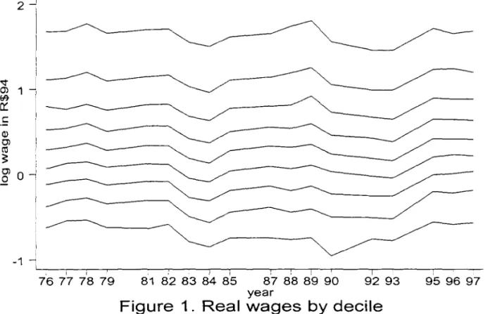
The information on trends in real log wages by decile provided by Figure 1

points to four periods of significant wage shifts. The first begins during the middle of

the 1981-83 recession with an 18.3 percent wage slide at the median in only two years,

perhaps also related to an almost doubling of the inflation rate from a monthly average of

4.7 percent from 1976 through 1982 to nine percent from 1983 to 1984.29 _{Wages then}

pick up from 1984 to 1989 in the context of declining unemployment and accelerating

inflation, which crosses the 50 percent a month threshold in December of 1989.

Furthermore, the aforementioned rise in wages is roughly positively correlated with

,

..

plans implemented from 1989 to 1993 has a negative impact on wages, which only

bounce back during the longer lasting low inflation years produced by the 1994 Real

Plano During this period the wages of the first six deciles reach their maximum, while

those of the top two deciles stabilize at slightly lower leveIs than their 1989 highs.

Overall, the median wage is 28.9 percent higher in 1997 than in 1993 and 13.5 percent

higher in 1997 than in 1976.

[F igure 1: Real wages by decile]

As Figure 2 shows, the largest relative wage changes occur at the extremes ofthe

wage distribution and most notably during three main stages: the high inflation years

1987 through 1989, then during the following attempts at inflation control, and finally

after the onset ofthe post 1994 price stable period. From 1987 to 1989, whence inflation

shot up to an average 32 percent monthly rate, the 90/20 and 80120 wage ratios rise 19.2

and 14 percent, respectively, to go dO\VTI by 20.6 and 13.5 percent from 1989 to 1993 and

then a further 10.7 and 12.1 percent from 1993 to 1997. The 90110 ratio follows an even

sharper trend with the exception that its fali occurs mostly from 1990 to 1992, a change

quite likely influenced by the fact that the minimum wage rose by 45.2 percent from

1990 to 1992 to go back do\VTI 1l.1 percent from 1992 to 1997 (See Section VII, Table

2). Comparatively, changes at the middle ofthe income distribution are rather limited,

and the smaller the closer to the mediano The 70/30 and 60/40 ratios go up 12.5 and 2.5

percent from 1987 to 1989, then do\VTI 14.3 and 5.6 percent from 1989 to 1993, to go

further do\'m by 5.4 and 1.2 percent from 1993 to 1997. In ali, during the 21-year time

period under consideration the 90/20,80/20, 70/30 and 60/40 ratios decline by 16.8,

•

that wage differentials are still a long ways away from those prevalent in developed

economies. A 199790110 ratio of9.5 compares very unfavorably with that of2.4

prevalent in The Netherlands, 2.5 in Germany, 3.1 in the United Kingdom or even the

ratio of a high inequality country such as the United States of 5.7. Similarly, a 80120

ratio of 4.3 is quite higher than that of the 1.4 found in The Netherlands, 1.8 in Germany,

2.1 in the United Kingdom and 3.0 prevalent in the United States.30

[Figure 2: Oecile ratios]

The use ofbetter measures ofwage dispersion alIows for a more precise gauge

of income distribution changes (Figure 3). The Gini, Theil and mean logarithmic

deviation (mld) indices, measures respecting the axioms of scale and population

independence, symmetry and the transfer principIe, showa fall in wage concentration of

3.9 to 12.7 percent during the mostly upward cyc1e 1976 to 1981, an increase of 1.3 to

five percent during the 1981-83 recession, a sharper rise of 6.1 to 15 percent during the

high inflation years, followed by a long lasting decline starting only around 1994. The

post 1994 drop ranges from 6.8 to 21.5 percent and the fact that the dov.nturn is greatest

for the Theil measure underscores the fact that relative wage changes were dominated by

movements at the top ofthe income distribution. In alI, wage inequality is 6.8 to 16.3

percent lower in 1997 than in 1976. Alternative measures of inequality such as the

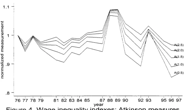
Atkinson indices (Figure 4), measures which also respect the aforementioned axioms,

follow similar patterns with their degree of change depending on how sensitive the index

is to inequality among higher incomes. For the post 1994 period, inequality alleviation

estimates range from 6.7 percent for the bottom sensitive A(2.5) index to 15 percent for

,

from a 3.7 to a 13.4 percent, measurements also underscoring the fact that changes were

dominated by movements at the higher end of the income distribution, as evidenced by

the larger inequality reduction estimates ofthe Atkinson indices with lower E values.

[Figures 3-4 and Table 1: Mld, Gini and Theil indexes]

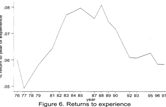
Final1y, a break up of the wage series into changes in worker characteristics and

their prices (Figures 5-6) shows a steady ascent of the col1ege premi um from 1977 to

1988 when a maximum is reached. Price stabilization plans have negative effects on the

differential, but an upward trend is resumed by 1992. Overal1, the col1ege to high school

wage premium reaches a considerable 83.9 percent by 1997. However, returns to lower

leveIs of education decline steadily throughout the time period under consideration, a

phenomenon perhaps related to the substantial drop in the percentage of workers with no

more than prima!)' education, which declined from 60.1 percent in 1976 to 36.9 percent

in 1997 (Figure 7). In turn, the price of experience increases rather steadily from 1977 to

1988 to decline thereafter. In al1, the premium is not much different in 1997 than in

1976- some six percent per annum. Lastly, residual inequality seems to rise with

increasing inflation and decline with price stability (Figure 8). The variance of the error

of a regression of the log wage on education, experience, sectoral and regional dummies

increases by 11 percent from 1982 to 1987, by 23.5 percent from 1987 to 1989, to

decline by 10.6 percent from 1989 to 1993 and then by a further 12.4 percent from 1993

to 1997.31

[Figures 5-8: Retums to education, experience, residual inequality, education]

It is then the purpose of the rest of the study to isolate the contributions of these

•

what extent are the changes in inequality related to a changing educational and

demographic profile of the population, to what extent are they due to changes in the

prices of these observed characteristics, and to what extent are they due to a changing

structure of unobserved characteristics and their prices. Such an exercise will not only

allow for an understanding of the direct contributors to the trends in wage distribution,

but may provide c1ues as to possible connections with other less obvious sources.

v.

Methodology

Juhn, Murphy and Pierce suggest a simple methodology for decomposing wage

distribution trends into contributions related to changes over time in worker

characteristics, skill prices, and leveIs and prices ofunobservable traits.32 _{The authors}

assume the usual wage equation with wages a function of observed worker

characteristics X, prices

13,

their prices, alternatively referred to as a residual for the sake ofbrevity. Central to the

method is the latter term' s expression as two components, one corresponding to a

cumulative distribution function of the residual and the second to an individual' s

percentile in the residual distribution. That is, ifFt·1eXit) is defined as year t's in verse

cumulative residual distribution for workers with characteristics Xit , and 8it as the

percentile of individual i' s residual in that distribution, Ft·I(8it

!

The wage generating equation can hence be expressed in the following manner.

•

distributions holding constant skill leveIs, prices or residual wage dispersion. A change

in wage distribution can then be divided into the three sources shown in equation two.

The first corresponds to the portion of a distributional change that can be attributed to a

varying structure of observed worker characteristics such as education or experience.

The second term amounts to the contribution of evolving skill prices such as the

--1

education or experience premia. Third, with F (-

I

average cumulative residual distribution, the last term tallies the contribution to a

distributional change attributable to varying residual dispersion.

In practice, the contributions of each of the components can be calculated in the

following manner. First, wages Y:_I (equation 3) are computed for the time periods

whose distributional change is to be decomposed. To do so, year t characteristics are

evaluated not at their corresponding years' prices, but at a mean price

J3

the average price over all time periods. In addition, the residual variance is held constant

by ca1culating an average cumulative residual distribution where, once again, the average

is over all time periods. Each person i in year t is then assigned a residual computed

--1

•

u's percentile corresponds to that in year t's residual distribution (Bit). Then, as both

prices and residuaIs are held constant in the distributions ofY:_{1 '} the difference in

inequality leveIs in both years can be interpreted as produced by a changing observed

worker characteristic structure.

(3)

(4)

(5)

To arrive at the contribution of changing prices, a second wage Y ｾ＠ (equation 4)

is constructed using year t characteristicsb year t prices, and a residual terrn computed as

in Y:₁• Hence, being that residuaIs are held constant in the distributions ofY ｾ＠ , any

additional change in inequality can then be attributed to a changing price structure for

observables. Lastly, to calculate the contribution of a changing residual distribution, a

third wage Y ｾｉ＠ (equation 5) is computed using year t characteristics, year t prices and a

residual constructed using year t's in verse cumulative residual distribution and year t's

•

ofthe years under consideration. Any remaining change in inequality can then be

attributed to changing residual variance.

VI. Empirical Aoalysis

The decomposition methodology is applied to the understanding of the factors

behind distributional shifts occurring during criticaI spells in the time period under

consideration. The first of these is encompassed by the years 1976 and 1980, which can

perhaps be categorized as ones of strong gwwth with modera te inflation. Between 1976

and 1980 national product increased at an average 7.2 percent annual grO\",th rate (Table

2) while inflation stood at a annual average of 58.2 percent. The 1981 to 1983 recession

defines a second period. The economy contracted by a total of 6.1 percent and

unemployment reached 6.7 percent. Inflation picked up in 1983 to an 154.7 yearly rate,

though it did not reach much higher leveIs until 1987. During this third period prices

increased by a factor of over 900, reaching annual inflation rates of 323.4 percent in

1987,819 percent in 1988, and l349.3 percent in 1989. While 1988 was a recessionary

year, product increased by 3.5 and 3.2 percent in 1987 and 1989, respectively, while

unemployment decreased from 3.8 to 3.3 percent from 1987 to 1989. Price stabilization

plans carne and went during the period 1989 to 1993, having temporary effects on

inflation and producing ups and dO\\lls in product and emp10yment. Long term price

annualized rate of some 12 percent from August 1994 to the end of 1997. Growth stood

at an average 4.2 percent per annum. Finally, in providing a context to the changes in

wage distribution, it must be pointed out that the value of the minimum wage eroded

from 1976 to 1990 when it reached a leveI equivalent to 56.3 percent of its 1976 value.

One then finds a marked 45.2 percent hike from 1990 to 1992, then a moderate slide

thereafter.

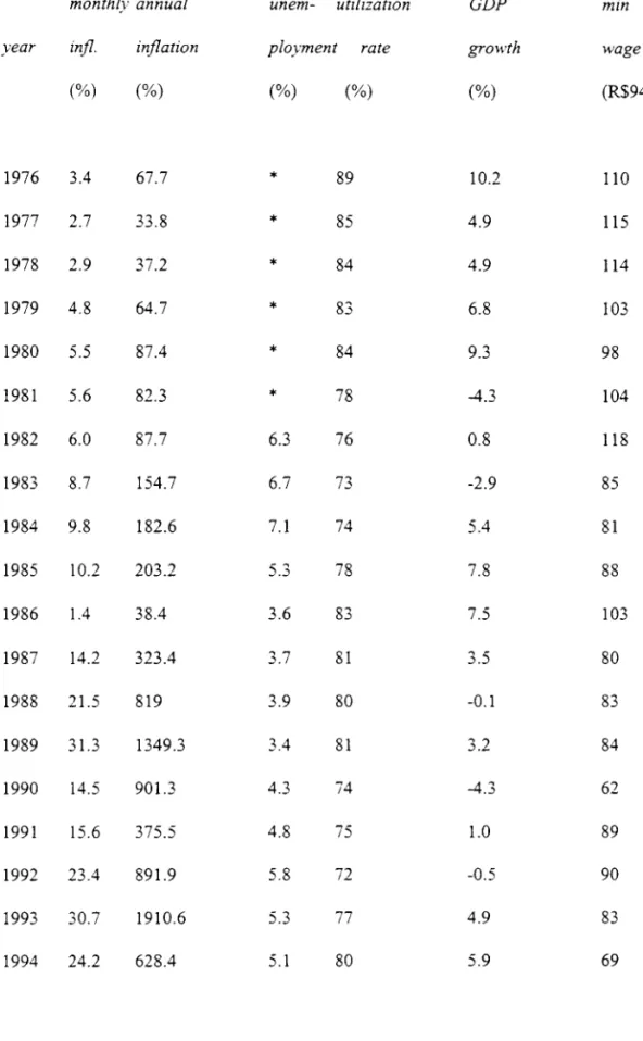
[Table 2: Macroeconomic indicators]

As touched upon in Section IV, the years 1976-1981 constitute a period where

inequality declined 3.9 to 12.7 percent, those between 1981 and 1983 correspond to an

increase of 1.3 to five percent, 1987 to 1989 to a rise of6.1 to 15 percent, and finally

1993 to 1997 to a slide of6.8 to 21.5 percent.33 _{In all, wage concentration declines by}

6.8 to 16.3 percent over a 21-year span, with changes dominated by movements at the top

ofthe distribution as in the case ofall subperiods. To arrive at an explanation ofthe

factors behind these events, a decomposition ofthe trends in to the often-mentioned

components is performed, with results sho'WTI in Table 3. In their computation, the

distributions of Y;, , Y ｾ＠ and ｙｾＬ＠ have been constructed as discussed in Section V. Then,

the Theil, Gini. and mld indices have been utilized to estimate the changes in the

dispersion of the exponential of wages in each of the distributions, differences from

which the decompositions derive.

[Table 3: Decompositions ofthe trend in wage distribution]

As the numbers show, changes are dominated by the unmeasured price and

occurring from 1976 to 1981 can be attributed to this phenomenon. Of the upsurge in

inequality occurring during the ensuing years (1981-83),59.4 to 69.6 percent can be

associated with rising residual dispersion, which in turn accounts for a considerable 77.6

to 88.8 percent of the jump occurring between 1987 and 1989. An also substantial 69.5

to 76.8 percent ofthe falI that took place between 1993 and 1997 can be identified with

this phenomenon.

This is not to say that the observable dimension's contribution is negligible.

From 1976 to 1981 an educational expansion that takes the form of an increment in the

proportion ofworkers with a high school or colIege diploma contributes to a rise in

inequality equivalent to 19.6 to 60.6 percent ofthe overall change. The effect is however

overwhelmed by a sharper fall in skilI prices, where declining college and high school

premia play a pivotal role (See Table 4). In net terms, the observed price and quantity

change is responsible for 2.5 to 29.6 percent of the reduction in wage dispersion.

Obsef\ables play a more prominent role during the 1981-83 recession, though skilI prices

work thls time in the opposite direction. Their contribution to higher leveIs of inequality

are eqU1\"alent to 26.8 to 35.1 percent ofthe total increase. Central to the component is

the upswing in the college and experience premia which rose markedly in only a

two-year span. For the remaining time periods, the influence of changing observables is more

subdued. From 1987 to 1989 an increase in skill prices boosted inequality leveIs by a

factor equivalent to 15.4 to 25 percent of the overall change, while during 1993-97 they

had almost no perceptible effect.

Results for the period 1976 to 1989 are consistent with those obtained by

Fishlow et. aI. and Bonelli and Ramos.34 _{In these studies the authors establish that a}

combination of demographic and between group inequality changes helped bring down

eamings dispersion during the latter half of the decade of the 1970s, increase inequality

during the recession of the early 1980s, and heighten inequality during the latter half of

the decade of the 1980s, though the importance of the factors during this last period is

not as great as in the earlier two. What this analysis adds to the discussion are the

following contributions to the story. First, changes in the residual distribution seem to

be more important in the determination of inequality changes than calculated in the cited

articles where less than 50 percent ofthe changes occurring during 1976-81 and 1981-83

are attributed to this factor. Part of the discrepancy lies in the fact that the studies

include in their sample wage eamers, employers and the self-employed and it is precisely

the variable associated with this distinction that which drives the importance ofthe

between group component, as can be leamed from the studies' tables. Thus, the

changing between-group inequality referred to by Fishlow et. aI. and Bonelli and Ramos

refers more to changing income differentials between the salaried, the self-employed and

employers than changing differences between educational and experience groupS.35

F urther details emerge when a variety of indices is used to decompose the trends

in inequality. Differing sensitivities to inequality at various segments ofthe distribution

allow one to conclude that observables are more important at the higher than the lower

end of the distribution where the unobservable' s contribution predominates. For

example, during 1976-81 the upperbound on the observed dimension's contribution

corresponds to the use of the mld index (2.5 percent). During the recession of the early

1980s 40.6 percent of the rise in inequality as measured by the Theil index can be

associated with observables, while the corresponding share comes down to 30.4 percent

when the mld index is used. The same occurs during the late 1980s when 22.4 percent of

the rise can be associated with observables from the point of view of the Theil index, but

a smalIer 11.1 percent when viewed through the rnld measure. For the decade ofthe

1990s the corresponding figures are 30.5 and 23.2 percent for the Theil and mld indices,

respectively.

A third contribution of this study is the extension of the analysis into the decade

of the 1990s, where price stabilization plans produced considerable swings in wage

dispersion and a general slide in real wage leveIs. Once prices stabilized, real wages

rose by 28.9 percent and dispersion declined by 6.8 to 21.5 percent. The driving force

behind the development is a considerable reduction in residual dispersion equivalent to

69.5 to 76.8 percent ofthe overalI change. Demographic shifts are responsible for the

balance of the falI. Together, both phenomena produce the largest sustained decline in

inequality experienced during the 21-year period under consideration. However, it is

important to note that there seem to be limits to the equality enhancing effects of price

stability, as can be reasonably expected. An initial drastic reduction in inequality

between 1993 and 1995 is followed by a much less pronounced falI between 1995 to

1996, and finalIy by constant to slightly increasing leveIs in 1997.

The fourth contribution of this study to the discussion of the factors behind the

evolution of inequality in Brazil is the clarification of the role played by education in

studies. The isolation of the effect of changing quantities from changing prices and the

extension into the decade ofthe 1990s allows for the following elements to emerge. As

can be ascertained in Table 4 or Figure 7, during the late 1970s the growth in education

took the forro of a shift from interroediate to higher learning. On the one hand, since the

educational expansion occurred from groups \vith wages closer to the mean to groups

with wages farther from the mean, the new distribution of education contributed to

higher leveIs ofbetween group inequality. Yet, on the other hand, the change had an

equalizing effect through skill prices, as reflected by the falling college and high school

premia. In net terros, the lower price for skill dominated the quantity effect to produce

an overall drop in inequality.

Comparatively, worker characteristic changes have much less impact during the

decade of the 1980s and are dominated by rising skill prices related first to the 1981-83

receSSion and then to the close to hyperinflationary context of the latter part of the

decade. A clue as to why did the price of skill rise during the recession lies in the fact

that ali wages declined during this period, yet, those of the college educated and the

experienced less so than others.36 _{Hence, the recession had its expected effect on wages,}

effect which was greater for the unskilled than the skilled for reasons perhaps having to

do with differences in protection against inflation. In just one year the 1983 minimum

wage stood at 72 percent of its 1982 value, with its corresponding effect on other low

skilled wages which are in many cases set in reference to the mentioned benchmark. On

the rise of the price of skill during the high inflationary period of the late 1980s, the

macroeconomic context not only seems to affect the variance ofthe prices of goods and

the price for unobservables, as manifested by the momentous two-year jump in residual

dispersion that took place from 1987 to 1989 (Figure 8). Finally, during the decade of

the 1990s observed prices take a back seat to observed quantities, which contrary to the

case of the decade of the 1970s, help reduce and not raise inequality. The explanation

lies in Table 4. Whereas during the decade ofthe late 1970s the educational expansion

takes the fonn of a shift from intennediate to higher education, that from 1993 to 1997

takes one from primary to intennediate. Since the price of intennediate education is

closer to the mean than that of primary education, the change in characteristic quantities

had the effect of decreasing between group inequality. Hence, a consistent role of

education emerges in this 21-year analysis of wage inequality in Brazil. Skill prices are

affected by demographics and the macroeconomic price context in sensible directions;

the effect on inequality of observed quantities depends on where the educational

expanslOn occurs.

[Table 5: Extended decompositions]

Yet another result that emerges from this study is that even over the longer run

unobservables still play a considerable role in the detennination of changes in inequality,

as evidenced in the bottom panel of Table 3. F orty-one point seven to 47.5 percent of the

6.8 to 16.3 percent decline in inequality experienced during the 21-year period under

analysis can be pinned to this source, this despite a concurrent and considerable change

in the distribution of education. The referred to phenomenon can be associated with the

remainder of the change, with the distribution of education having a small but negative

effect on inequality that is overwhelmed by a much larger positive trend in observable

leveIs of education recede significantly during the same period. Hence, Lam and

Levison' s optimism on the long lasting effects of a reduction in schooling inequality

experienced from 1976 to 1985 has proven to be well founded.37

However, as

manifested by the comparatively high leveIs of inequality still prevalent in Brazil, there

remains much room for progresso

Finally, questions may arise as to the long-run effects on distribution of changes

in the sectoral composition ofthe Brazilian economy. To that end, the 1976 to 1997 time

period is decomposed using a regression which includes, besides education and

experience variables, eight sector dummies. Results shown in Table 5 attest to the fact

that the new variables add very little explanatory power to the decomposition.

According to the rnld and Gini indices, the amount of the variation that is explained by

the observable dimension increases from 58.3 and 59.3 percent to 59.2 and 62.0 percent,

respectively. Sectoral developments are slightly more important at the higher end ofthe

distribution, as manifested by the fact that the largest increase in explanatory power

occurs when the Theil index is used to measure distributional changes. However, even

in this case the addition ofthe binary variables raises the contribution of obser\'ables

from 52.5 to 57.7 percent. Hence, the sectoral trend from manufacturing to services that

occurred in Brazil during the period under study does not seem to be at the center of the

tendencies in inequality. Explanations lie elsewhere, including changing skill prices, and

more importantly, changing residual dispersion which appears to be particularly

susceptible to the macroeconomic price context.

Wage dispersion in Brazil fluctuates considerably during the period under study.

An annualized decline of some .8 to 2.4 percent during the late 1970s is folIowed by an

annualized rise of.5 to 2.5 percent during the 1981-83 recession and then by a further

three to 7.2 annualized rate during the cIose to hyperinflationary 1987-89 period. In alI,

wage inequality grows by up to an impressive 20 percent during the decade ofthe 1980s.

A series of stabilization programs produces wild swings in wage distribution which end

only with the 1994 Real Plano During this period not only does the median wage

increase by some 29 percent, but abso1ute changes favor those at the 10wer end of the

distribution. That is, while wages at the bottom six deciles reach a 21-year maximum,

those at the top two drop re1ative to their peaks in 1989. The result is a significant falI in

wage dispersion of some seven to 22 percent. Overall, inequality recedes by seven to 16

percent from 1976 to 1997, change characterized by considerable real wage advances at

the lower half of the distribution.

A decomposition analysis performed to ascertain the source of these events

places changes in quantities and prices ofunobservable skilI at the center ofthe short

term trends in inequality. At their maximum degree of influence they are responsible for

78 to 89 percent of the deep hike in inequality occurring during the high inflation period

of the latter part of the 1980s. At their minimum they account for 59 to 70 percent of the

rise occurring during the ear1y part ofthe decade. Far behind in importance in the

determination of short-run trends are price and quantity changes of observable skilI.

Prices first seem to react to significant shifts in the educational composition ofthe

macroeconomic price context- rising with creeping inflation and dropping with price

stability. Observed quantities, particularly education, follow a more consistent pattem

with their effect on distribution depending on where does the educational expansion

occurs- advancements into higher education ha,ing negative effects on distribution while

advances into intermediate leveis having positive consequences. Only over a longer run

does the observable dimension play a more significant role in the determination of

inequality trends. Fifty-two to 59 percent ofthe drop in inequality occurring between

1976 to 1997 can be associated with changing quantities and prices of observed skill,

particularly education.

However, these hard eamed positive steps towards a more equal wage

distribution can become overwhelmed in a hurry in an unstable price context. With

inflation under some check during the late 1970s, demographic trends were able to have

a positive impact on inequality. Rising inflation rates during the early and middle 1980s

coincide with a step up of inequality, particularly its residual component. Close to

hyperinflationary leveIs jack up inequality during 1987-89 to extremely high leveis while

stabilization plans produce wild swings in dispersion during the ensuing years.

Inequality finally settles, and on much lower leveIs, only under the context ofprice

stability. However, while producing a marked decline in dispersion, a low inflationary

context seems to have its limits on distribution. The equality enhancing effects of

stability brought forth by the Real Plan seem to have run their course after two

consecutive years of inequality reduction. Yet, in view of the historic trends in Brazilian

distribution, even constant leveIs of inequality are achievements that cannot be dismissed

expected to increase dispersion.

As to other general implications ofthe results ofthis study, the high inflation

conditions that characterize much of the period under study make it difficult to draw too

many comparisons with the case of other countries. While inequality declined during the

late 1970s and rose consistently during the decade of the 1980s as in the case of many

other economies, the factors related to the latter decade's increased dispersion are quite

different from those driving up inequality in most of the developed world. Still, this

research does confirrn that the college premium did decline in Brazil during the late

1970s and then grew thereafter rather continuously as in the case of many other

countries. AIso, as concluded in studies investigating the source of distributional trends

in developed economies, sectoral shifts do not seem to be at the center of changes in

inequality in BraziI. Residual distributional phenomena not only seem to dominate

short-run trends but also play a substantial role in longer terrn ones.

NOTES

1. See Peter Gottchalk and Timothy Smeeding, "Cross-National Comparisons of

Earnings and Income Inequality," Journal ofEconomic Literature, voI. 35, no. 2

(June 1997): 633-87 for a survey of the literature.

2. See Sebastian Edwards, Crisis and Reforrn in Latin America: From Despair to Hope

(Oxford and New York: Oxford University Press and the World Bank, 1995) for an

in-depth description of the policy changes.

Review, vo1. 62, no. 2 (May 1972): 391-402.

4. Rodolfo Hoffmann and J. Duarte, "A Distribuição da Renda no Brasil" (Income

Distribution in Brazil), Revista de Administração de Empresas, vo1. 12, no. 2 (June

1972): 46-66; Carlos Langoni, Distribuição de Renda e Desenvolvimento

Econômico do Brasil (Income Distribution and Economic Development in Brazil)

(Rio de Janeiro: Expressão e Cultura, 1973).

5. Gary Fields, "Who Benefits from Economic Development? A Reexamination of

Brazilian Growth in the 1960's," American Economic Review, vo1. 62, no. 4

(September 1977): 570-82.

6. Montek Ahluwalia, John Duloy, Graham Pyatt and T. Srinivasan, "Who Benefits

from Economic Development?: Comment," American Economic Review, vo1. 70,

no. 1 (March 1980): 242-45; Paul Beckerrnan and Donald Coes, "Who Benefits

from Economic Development?: Comment," American Economic Review, vo1. 70,

no. 1 (March 1980): 246-49; Albert Fishlow, "Who Benefits from Economic

Development?: Comment," American Economic Review, vo1. 70, no. 1 (March

1980): 250-56.

7. Fishlow, "Who Benefits from Economic Development?: Comment" (n. 6 above).

8. Gary Fields, "Who Benefits from Economic Development?: Reply," American

Economic Review, vo1. 70, no. 1 (March 1980): 257-62.

9. Lance Taylor, Edmar Bacha, Eliana Cardoso and Frank Lysy, Models ofGro\\th and

Distribution for Brazil (Oxford: Oxford University Press, 1980).

11. Ibid.

12. Fishlow, "Brazilian Size Distribution ofIncome" (n. 3 above); Rodo1fo Hoffmann,

"Considerações Sobre a Evolução Recente da Distribuição da Renda no Brasil"

(Considerations on the Recent Evolution of Income Distribution in Brazil), Revista

de Administração de Empresas, vo1. 13, no. 4 (October-December 1973): 7-17.

13. Albert Fishlow, "Distribuição da Renda no Brasil: um Novo Exame" (Brazilian

Income Size Distribution: Another Look), Dados, vo1. 11, (1973): 10-80; Edmar

Bacha, Os Mitos de uma Década: Ensaios de Economia Brasileira (Myths of a

Decade: Essays on the Brazilian Economy) (Rio de Janeiro: Paz e Terra, 1976).

14. Edmar Bacha and Lance Taylor, "Brazilian Income Distribution in the 1960s:

'Facts,' Model Results and the Controversy," Models of Growth and Distribution for

Brazil, ed. Lance Taylor, Edmar Bacha, Eliana Cardoso and Frank Lysy, (Oxford:

Oxford University Press, 1980).

15. Rodolfo Hoffmann and Angela Kageyama, "Distribuição da Renda no Brasil, Entre

Famílias e Entre Pessoas, em 1970 e 1980" (Individual and Family Income

Distribution in Brazil in 1970 and 1980), Estudos Econômicos, vo1. 16, no. 1

(January-Apri1 1986): 25-51.

16. Regis Bonelli and Lauro Ramos, "Distribuição de Renda no Brasil: Avaliação das

Tendencias de Longo Prazo e Mudanças na Desigualdade desde Meados dos Anos

70" (Income Distribution in Brazil: Appraisal of Long Run Trends and Changes in

Inequality since the Mid-1970s), Revista Brasileira de Economia, vo1. 49, no. 2

(April-June 1995): 353-73.

na Argentina: uma Análise Comparativa" (Income Distribution in Brazil and

Argentina: A Comparative Analysis), Pesquisa e Planejamento Econômico, vo1. 23,

no. 1 (April 1993): 1-31.

18. Bonelli and Ramos (n. 16 above).

19. Fishlow, Fiszbein and Ramos (n. 17 above).

20. Bonelli and Ramos (n. 16 above).

21. Rodolfo Hoffrnann, "Desigualdade e Pobreza no Brasil no Período 1979-90"

(Inequality and Poverty in Brazil during the 1979-90 Period), Revista Brasileira de

Economia, vo1. 49, no. 2 (April-June 1995): 277-94.

22. Fishlow, "Brazilian Size Distribution ofIncome" (n. 3 above); Langoni (n. 4

above); J. Senna, "Escolaridade, Experiência no Trabalho e Salários no Brasil"

(Schooling, Work Experience and Wages in Brazil), Revista Brasileira de Economia,

vo1. 30, no. 2 (April-June 1976): 163-93; R. Castello Branco, Crescimento

Acelerado e Mercado de Trabalho: A Experiência Brasileira (Rapid Grow1h and the

Labor Market: the Brazilian Experience) (Rio de Janeiro: Getulio Vargas

Foundation, 1979); Jacques Velloso, "Educação e Desigualdade da Renda Urbana

no Brasil: 1960/80" (Education and Income Inequality in Urban Brazil: 1960/80),

Pesquisa e Planejamento Econômico, vo1. 9, no. 3 (December 1979): 661-718.

23. José Reis and Ricardo Barros, "Wage Inequality and the Distribution ofEducation,"

Joumal ofDevelopment Economics, vo1. 36, no. 1 (July 1991): 117-43.

24. David Lam and Deborah Levison, "Declining Inequality in Schooling in Brazil and

its Effects on Inequality in Eamings," Joumal ofDevelopment Economics, vo1. 37,

25. Nineteen-eighty six wil! however be excluded from the study since it was a year of

drastic but ephemeral changes produced by the Cruzado Plano On this see Regis

Bonelli and Guilherme Sedlacek, "A Evolução da Distribuição da Renda entre 1983

e 1988" (The Evolution of Income Inequality between 1983 and 1988), Distribuicão

de Renda no Brasil (Income Distribution in Brazil), ed. J. Camargo and F. Giambiagi

(Rio de Janeiro: Paz e Terra, 1991) and Hoffmann, "Desigualdade e Pobreza no

Brasil no Período 1979-90" (n. 21 above).

26. Fishlow, Fiszbein and Ramos (n. 17 above); Lam and Levison (n. 24 above); Reis

and Barros (n. 23 above).

27. Hoffmann, "Desigualdade e Pobreza no Brasil no Período 1979-90" (n. 21 above).

28. Fishlow, Fiszbein and Ramos (n. 17 above); Bonelli and Ramos (n. 16 above).

29. See Table 2 in Section VI for a macroeconomic contexto

30. The developed economies' decile ratios are found in Gottshalk and Smeeding (n. 1

above), Table 1. These are however constructed from earnings, not wages. Ifthe

same is done for Brazil, the 1997 90/1 O and 80/20 ratios are stil! a considerable 9.4

and 3.8, respectively. AIso, European and American statistics are based on

distributions from the mid 1980s to early 1990s.

31. The education and experience premia are derived from the same type of equation.

The latter is evaluated at ten years of experience.

32. Chinhui Juhn, Kevin Murphy and Brooks Pierce, "Wage Inequality and the Rise in

Returns to Skill," Journal ofPolitical Economv, vo1. 101, no. 3 (June 1993):

410-42.

1980 Pnad data is not available, 1981 will be taken as the ending year reference in

the decomposition. Its choice is convenient for comparative purposes since other

studies also use it as reference year.

34. Fishlow, Fiszbein and Ramos (n. 17 above); Bonelli and Ramos (n. 16 above).

35. Ibid.

36. From 1981 to 1983 the average wage ofthe college educated fell by 14 percent while

that of the high school graduate tumbled by 20 percent. The wage of the college

graduate with 20 years of experience dropped by 13 percent while that of the

graduate with tive years of experience did so by 22 percent.

37. Lam and Levison (n. 24 above).

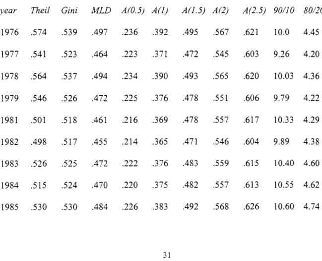
Table 1. Wage inequality by index

year Theil Gini MLD A(O.5) A(l) A(l.5) A (2) A (2. 5) 90/10 80/20

1976 .574 .539 .497 .236 .392 .495 .567 .621 10.0 4.45

1977 .541 .523 .464 .223 .371 .472 .545 .603 9.26 4.20

1978 .564 .537 .494 .234 .390 .493 .565 .620 10.03 4.36

1979 .546 .526 .472 .225 .376 .478 .551 .606 9.79 4.22

1981 .501 .518 .461 .216 .369 .478 .557 .617 10.33 4.29

1982 .498 .517 .455 .214 .365 .471 .546 .604 9.89 4.38

1983 .526 .525 .472 .222 .376 .483 .559 .615 10.40 4.60

1984 .515 .524 .470 .220 .375 .482 .557 .613 10.55 4.62

1987 .523 .525 .478 .223 .380 .491 .571 .631 11.00 4.62

1988 .604 .558 .549 .253 .423 .537 .616 .676 12.34 5.14

1989 .601 .557 .549 .252 .422 .537 .617 .677 12.83 5.26

1990 .502 .517 .470 .221 .381 .497 .582 .646 12.39 4.74

1992 .495 .509 .448 .211 .361 .471 .555 .622 9.19 4.48

1993 .613 .539 .503 .241 .395 .501 .579 .641 9.38 4.55

1995 .509 .514 .454 .215 .365 .471 .548 .608 9.74 4.20

1996 .468 .499 .428 .202 .348 .456 .537 .600 9.45 4.31

);ear 1976 1977 1978 1979 1980 1981 1982 1983 1984 1985 1986 1987 1988 1989 1990 1991 1992 1993 1994

Table 2. Macroeconomic indicators and minimum wage, Brazi11976-97

monthly annual

injl. (%) 3.4 2.7 2.9 4.8 5.5 5.6 6.0 8.7 9.8 10.2 1.4 14.2 21.5 31.3 14.5 15.6 23.4 30.7 24.2 injlation (%) 67.7 33.8 37.2 64.7 87.4 82.3 87.7 154.7 182.6 203.2 38.4 323.4 819 1349.3 901.3 375.5 891.9 1910.6 628.4 unem- utilization

ployment rate

(%) (%)

*

*

*

*

*

*

6.3 76 6.7 73 7.1 74

5.3 78 3.6 83 3.7 81

3.9 80 3.4 81 4.3 74 4.8 75 5.8 72

5.3 77 5.1 80

1995 1.6

1996 0.6

1997 0.3

20.2

7.5

3.5

4.6

5.4

5.7

83 82 84

4.2

2.8

3.7

79

78

80

Source: Inflation rates are based from 1976 to 1979 on the IGP-DI found in Conjuntura

Econômica of the Fundação Getulio Vargas, and from 1979 to 1997 on the INPC found

in the Anuario Estatístico from Instituto Brasileiro de Geografia e Estatística. Utilization

and GDP growth rates are found in Conjuntura Econômica. (*) Unemployment rates are

drawn from the Monthly Employment Survey carried out since 1982 by the Instituto

Brasileiro de Geografia e Estatística. The nominal minimum wage comes from the Folha

de São Paulo, as found in Macrometrica time series, and real rates are produced using the

aforementioned concatenated price indexo Conversions are carried out according to the

lndex

rnld

Gini

Theil

rnld

Gini

Theil

Table 3. Decomposition of the trend in wage inequality Experience and education variables

Total

Quantities + Prices + Residual = Change

(percent 01 total change)

1976-81

.0220 -.0229 -.0354 -.0363

(60.6) (-63.1) (-97.5) (-100)

.0098 -.0l30 -.0178 -.0210

(46.7) (-61.9) (-84.8) (-100)

.0143 -.0359 -.0514 -.0730

(19.6) (-49.2) (-70.4) (-100)

1981-83

.0004 .0030 .0078 .0112

(3.6) (26.8) (69.6) (100)

.0003 .0022 .0041 .0066

(4.5) (33.3) (62.1) (100)

.0014 .0088 .0149 .0251

(5.6) (35.1) (59.4) (100)

Total

lndex Quantities + Prices + Residual = Change

(percent of total change)

1987-89

rnld -.0030 .0109 .0629 .0708

(-4.2) (15.4) (88.8) (100)

Gini -.0012 .0058 .0276 .0322

(-3.7) (18.0) (85.7) (100)

Theil -.0020 .0196 .0609 .0785

(-2.5) (25.0) (77.6) (100)

1993-97

rnld -.0154 -.0011 -.0546 -.0711

(-21.7) (-1.5) (-76.8) (-100)

Gini -.0091 -.0001 -.0273 -.0365

(-24.9) (-0.3) (-74.8) (-100)

Theil -.0418 .0016 -.0916 -.1318

Table 3- Continued

Total

lndex Quantities + Prices + Residual = Change

(percent of total change)

1976-97

mld .0142 -.0523 -.0273 -.0654

(21.7) (-80.0) (-41.7) (-100)

Gini .0038 -.0256 -.0150 -.0368

(10.3) (-69.6) (-40.8) (-100)

Theil .0057 -.0547 -.0444 -.0934

Table 4. Skill premia and distribution of education

premium (%) 1976 1981 1983 1987 1989 1993 1997

intennediate to primary 42.0 44.1 47.8 42.4 40.3 33.7 32.2

hs diploma to intennediate 79.6 67.0 66.8 65.8 70.3 62.8 60.9

college to hs dropout 116.8 111.5 114.3 120.4 124.3 110.6 118.2

college to hs diploma 78.1 72.7 78.7 84.0 88.1 82.2 83.9

expenence 6.00 6.44 7.71 7.57 7.45 6.07 5.83

population by

educationallevel (%) 1976 1981 1983 1987 1989 1993 1997

zero 13.5 12.3 10.6 10.1 9.2 7.5 6.7

pnmary 46.6 47.8 46.3 42.4 40.0 35.6 30.2

intennediate 21.1 16.8 17.7 19.7 21.7 25.2 28.5

secondary 3.2 3.0 3.0 3.9 4.3 4.7 4.8

secondary diploma 6.4 9.6 10.9 12.4 13.2 15.9 18.0

college 9.3 10.5 11.4 11.6 11.6

_ill

100 100 100 100 100 100 100

Note. The educational premi um is computed through the use of coefficients derived

from a regression ofthe log wage on education, experience, regional and sectoral

variables. Educationallevel figures correspond to the percentage of the sample attaining

Index

rnld

Gini

Theil

Table 5. Decomposition of the trend in wage inequality Experience, education and sectoral variables

Quantities + Prices + Residual = Change

(percent of total change)

1976-97

.0140 -.0527 -.0267 -.0654

(21.4) (-80.6) (-40.8) (-100)

.0038 -.0266 -.0140 -.0368

(10.3) (-72.3) (-38.0) (-100)

.0033 -.0572 -.0395 -.0934

2

't Ol l:F7 1

cr

C

Q)

Cl Cil

ｾ＠

8'

i

! I

I

-1

ＱｾｾＭＭＧＭＭｲＭＭＭＭＭＭＭｲＭＭＭＭｾＭＭＭＭＭＭｲＭｾｾＭＭｲＭＭＭＭＧＭＧＭＭＭＭＭｲｾＭＭＭＭ

76 77 78 79 81 82 83 84 85 87 88 89 90 92 93 95 96 97 year

Figure 1. Real wages

by

decile

l-a>

"O

(/)

a> ·ü a>

"O

15

g>

"O

C

O

a.

(/)

a>

....

....

O ü 5

....

O

(/)

O

...

C\l

....

o

---"'11120

---°"'2o

ＭＭＭＭＭＭＭＭＭＭＭＭＭＭＭＭＭＭＭＭＭＭＭＭＭＭＭＭＭＭＭＭＭＭＭＭＭＭＭＭＭＭＭＭＭＭＭＭＭＭＭＭｾＷｾｗＳＰ＠

60/40

I I I I I I I

76 77 78 79 81 82 83 84 85 87 88 89 90 9293 95 96 97 year

1.1

....

Q)

E

Q)

:s

fi) t1l

Q)

E

"O

Q)

N

tU .9

E

...

o

c

NI

i

I

.8 -i

ＭＭｾＭＭｾｾＬＭＭＭＭＧｉＭＭＧｉＭＭｾＬ＠ ｾＭＭＭＭＭＭＭＭＭＧＭＭｲＭＭＭＭＭｾＬＭＭｾＬＭＭＭＭＧｩＭＧＭＭＭＭ

76 77 78 79 81 82 83 84 85 87 88 89 90 92 93 95 96 97 year

1.1

J

-

Q)

E

ｾ＠ 1

:::J

C/)

ro

Q)

E

"O

Q)

N

ｾ＠

.9l

o ,

c

Ii

.8 --j

.5) .0) .5)

ｾＮＵＩ＠

L ' - - , ' - - ' ,

--r,

76 77 78 79 81 82 83 84 85 87 88 89 90 92 93 95 96 97

year

ãi _> 1 ｾ＠

I

Q) I

CU

C

O :.;::;

ｾ＠ .8

::J "tl

Q)

Cl

ｴＶｾ＠

> .4 I

O i _,

c ｾ＠ i

"ê

LL

- - - -_ _ _ ..I::lS

R

ｾ＠ ＮＲｾｌｉ＠

ＭＭＧｉＭＭｲＭＧＭＭＭＧＭｾｉ＠

ＭＭＧｉＭＭＭＭＭＭｾＭＬＺＭＺｲＭＭＭＬｉＭＬＭＭｾｉＭｔｉＭｾ＠

76 77 78 79 81 82 83 84 85 87 88 89 90 92 93 95 96 97 year

a.>

u c

a.> ·C

.08

ｾ＠

a.> ,

C. :

X

.07-a.>

...

O

ｾ＠

ro

a.>

>-.8

:

ｾ＠ ,

::l

-

ｾ＠

":!2.

o

I

.05

J

/

\

I I I , I I I I I I I

76 77 78 79 81 82 83 84 85 87 88 89 90 92 93 95 96 97 year

-ai

ｾ＠ .6-1

c

O

:;:; co

U

:::J

"O

Q)

Cl .4 ｾ＠ C "O C

O

Q. til

ｾ＠

I

ｩＲＧｾ＠

Õ.

ｾ＠

=

E _co til

:::R

o

0-ｾｉＭＭｾｾｉＭＭＭＭＭＭＭＭＭＭｾｾＭＭｾｉＭＭｾｉＭＭＭＭｾＭＧｉＭＭｾｉＭＭＭＭＭＭｾＬＭＭｾｉＭＭＭＭｾＭＭＭＭＧＭ

76 77 78 79 81 82 83 84 85 87 88 89 90 92 93 95 96 97 year

00-oro

._ ::l

1.2

--o

ｾｾ＠

·u ...

Q)O -OQ) -OU Q) C

ｎＮｾ＠ 1

.-

...

-ro

ro >

E-o

Oc

cro

, I I I j

76 77 78 79 81 82 83 84 85

l

/

\

t \

ｾｍ＠

I I I ,

87 88 89 90 9293 year

Figure 8. Residual inequality

I I I

FUNDAÇÃOGETULlOVARGAS

BIBLIOTECA

ESTE VOLUME DEVE SER DEVOLVIDO À BIBLIOTECA NA ÚLTIMA DATA MARCADA

'i.Cham. P/EPGE SPE S718e

Autor: Sotomayor. Orlando J

Título: The evolution of wage inequality in Brazil. 1976 to