RESEARCH ARTICLE
A New Algorithm to Optimize Maximal
Information Coefficient
Yuan Chen1☯, Ying Zeng2☯, Feng Luo1,3,4
*, Zheming Yuan1,5*
1Hunan Provincial Key Laboratory for Biology and Control of Plant Diseases and Insect Pests, Hunan Agricultural University, Changsha, China,2Orient Science &Technology College of Hunan Agricultural University, Changsha, China,3College of Plant Protection, Hunan Agricultural University, Changsha, China, 4School of Computing, Clemson University, Clemson, South Carolina, United States of America,5Hunan Provincial Key Laboratory for Germplasm Innovation and Utilization of Crop, Hunan Agricultural University, Changsha, China
☯These authors contributed equally to this work.
*[email protected](FL);[email protected](ZY)
Abstract
The maximal information coefficient (MIC) captures dependences between paired vari-ables, including both functional and non-functional relationships. In this paper, we develop a new method, ChiMIC, to calculate the MIC values. The ChiMIC algorithm uses the chi-square test to terminate grid optimization and then removes the restriction of maximal grid size limitation of original ApproxMaxMI algorithm. Computational experiments show that ChiMIC algorithm can maintain same MIC values for noiseless functional relationships, but gives much smaller MIC values for independent variables. For noise functional relationship, the ChiMIC algorithm can reach the optimal partition much faster. Furthermore, the MCN values based on MIC calculated by ChiMIC can capture the complexity of functional rela-tionships in a better way, and the statistical powers of MIC calculated by ChiMIC are higher than those calculated by ApproxMaxMI. Moreover, the computational costs of ChiMIC are much less than those of ApproxMaxMI. We apply the MIC values tofeature selection and obtain better classification accuracy using features selected by the MIC values from ChiMIC.
Introduction
Identifying relationships between variables is an important scientific task in exploratory data mining [1]. Many measures have been developed, such as Pearson correlation coefficient [2], Spearman rank correlation coefficient, Kendall coefficient of concordance [3], mutual informa-tion estimators [4],[5],[6], distance correlation (dCor) [7], and correlation along a generating curve [8]. Recently, Reshefet al. [9] proposed a novel maximal information coefficient (MIC) measure to capture dependences between paired variables, including both functional and non-functional relationships [10],[11]. The MIC value has been applied successfully to many prob-lems [12–20]. The MIC of a pair of data seriesxandyis defined as follow:
MICðx;yÞ ¼maxfIðx;yÞ=log2minfnx;nygg ð1Þ
whereI(x,y) is the mutual information between dataxandy. Thenx,nyare the number of bins a11111
OPEN ACCESS
Citation:Chen Y, Zeng Y, Luo F, Yuan Z (2016) A New Algorithm to Optimize Maximal Information Coefficient. PLoS ONE 11(6): e0157567. doi:10.1371/ journal.pone.0157567
Editor:Zhongxue Chen, Indiana University Bloomington, UNITED STATES
Received:February 25, 2016
Accepted:June 1, 2016
Published:June 22, 2016
Copyright:© 2016 Chen et al. This is an open access article distributed under the terms of the Creative Commons Attribution License, which permits unrestricted use, distribution, and reproduction in any medium, provided the original author and source are credited.
Data Availability Statement:All relevant data are within the paper and its Supporting Information files.
into whichxandyare partitioned, respectively. Reshefet al. [9] developed a dynamic program algorithm, ApproxMaxMI, to calculate the MIC. As the bin sizes affect the value of mutual information, determining the appropriate value ofnxandnyis important. In ApproxMaxMI
algorithm, Reshef set thenx×ny˂B(n), whereB(n) =n0.6is the maximal grid size restriction and
nis the sample size. The generality of MIC is closely related toB(n). SettingB(n) too low will result in searching only for simple patterns and weakening the generality, while settingB(n) too high, will result in nontrivial MIC score for independent paired variables underfinite sam-ples. For example, the MIC value of two independent variables with 400 sample points calcu-lated by ApproxMaxMI is 0.15±0.017 (B(n) =n0.6, 500 replicates). Furthermore, the
computation cost of ApproxMaxMI becomes expensive when the sample sizenis large, which makes it difficult to calculate the MIC for big data.
Many efforts have been committed to improve the approximation algorithm for MIC by either optimizing the MIC value or reducing the computing time. Tanget al. [21] have pro-posed a cross-platform tool for the rapid computation of the MIC based on parallel computing methods. Wanget al. [22] have used quadratic optimization to calculate the MIC. Albanese et al. [23] re-implemented the ApproxMaxMI using C.[9]. Zhanget al. [10] have applied the simulated annealing and genetic algorithm, SGMIC, to optimize the MIC. Although SGMIC can achieve better MIC values, it is much more time-consuming.
In this paper, we develop a new algorithm to improve the MIC values as well as reduce the computational cost. Our new algorithm, ChiMIC, uses the chi-square test to determinate opti-mal bin size for the calculating of MIC value. Experiments on simulated data with different relationships (e.g. statistically independent, noiseless functional and noisy functional relation-ships) and real data show that our method can optimize the MIC value and significantly reduce the computation time.
Results
Comparison of MIC values for independent and noiseless functional
relationships
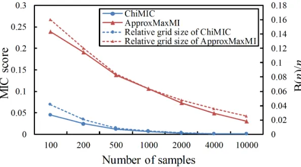
Ideally, the MIC values should be close to 0 for two independent variables. The MIC values for two independent variables calculated by ApproxMaxMI depend on the ratio between B(n) and n[24]. The MIC value for two independent variables is close to 0 only whennapproaches infinity, namely, the B(n)/ntrends to 0. Although, the MIC values calculated by ChiMIC also depend onB(n)/n, the ChiMIC algorithm gives much smaller MIC values for independent vari-ables and converges to zero faster as shown inFig 1. Specifically, for small sample sizes, the MIC values calculated by ChiMIC are much smaller. For example, when sample size is 100, MIC value calculated by ChiMIC is 0.06, while MIC value calculated by ApproxMaxMI is 0.24.
Meanwhile, the MIC values of two variables with noiseless functional relationships should be close to 1. We calculate the MIC values between variables with 21 different noiseless func-tional relationships (S1 Fig) using ChiMIC algorithm. All MIC values are equal to 1 as shown inS1 Table, which indicates that the ChiMIC algorithm maintains the generality of MIC.
Comparison of grid partition for noisy relationships
For noise relationships, the ChiMIC algorithm terminates the grid partition search much ear-lier than ApproxMaxMI. As shown inFig 2, both ChiMIC and ApproxMaxMI capture a noise-less linear relationship with a 2×2 grid (Fig 2A). When adding noise, the ApproxMaxMI partitions the noisy linear relationship with a 2×32 grid (Fig 2B). Meanwhile, ChiMIC parti-tions the noisy linear relaparti-tionship with just a 2×4 grid (Fig 2C). We also compare the grid
partition for parabolic function (Fig 3) and sinusoidal function (Fig 4). As shown in Figs3and
4, the ChiMIC algorithm partitions the noisy functional relationship into much fewer numbers of grids. The fewer numbers the grid are partitioned, the smaller the MIC values are calculated. The MIC values calculated by ChiMIC algorithm are always smaller than those calculated by ApproxMaxMI. We calculate the MIC values for 21 functional relationships with different noise levels (S2 Table). The higher the noise level, the smaller the MIC values calculated by ChiMIC comparing to those calculated by ApproxMaxMI.
Comparison of minimum cell number (MCN) estimation
In maximal information-based nonparametric exploration statistics, the minimum cell number (MCN) is the number of grid cells needed to calculate MIC values. It is defined as follows [24]:
MCNðD;εÞ ¼minflog2ðxyÞ:MðDÞx;y ð1 εÞMICðDÞg xy<B
ð2Þ
Fig 1. MIC values calculated by ApproxMaxMI and ChiMIC for random data with different sample sizes.The scores are reported as means over 500 replicates.
doi:10.1371/journal.pone.0157567.g001
Fig 2. Grid partition of ApproxMaxMI and ChiMIC for linear function.1000 data points simulated for functional relationships of the formy=x+η. whereηis noise drawn uniformly from (−0.25, 0.25). A: Grid partition for noiseless
linear function. B: Grid partition based on ApproxMaxMI for noisy linear function. C: Grid partition based on ChiMIC for noisy linear function.
doi:10.1371/journal.pone.0157567.g002
whereDis afinite set of ordered paired data. The parameterεprovides robustness for MCN.
This measure captures the complexity of the association between two variables. A greater MCN measure indicates a more complex association.
For independent variables, MCN is equal to 2 and is unrelated to sample size. Whenεis set
to 0, the MCN measure based on MIC calculated by ApproxMaxMI increases steadily as the sample size grows (Fig 5). Whenεis set to 1-MIC(D) as in Reshef [24], the MCN measures
based on MIC calculated by ApproxMaxMI algorithm do not increase as sample size grows, but still maintain greater than 3. On the other hand, the MCN values based on MIC calculated by ChiMIC are always close to 2.
For noiseless linear, parabolic and sinusoidal functions, the MCN values are 2, 2.58 and 3, respectively, for MIC calculated by either ApproxMaxMI or ChiMIC (Fig 6). As MCN values increase as the complexity of functional relationships increases, the MCN values should increase when weak noise is added. However, when the level of noise blurs the real functional relationship, the MCN values should decrease and converge towards 2. Thus, the MCN values should follow a parabolic graph as the noise level increases. We examine the MCN values when different levels of noise are added to linear, parabolic and sinusoidal functions. Whenεis set to
0 and noise level is greater than or equal to 0.4, the MCN values based on MIC calculated by ApproxMaxMI are always equal to 6 for all three functions (Fig 6A). Thus, MCN can no longer capture the complexity of functional relationships in this case. Whenεis set to 1-MIC(D),
only the MCN values based on MIC calculated by ApproxMaxMI for linear function follow the Fig 3. Grid partition of ApproxMaxMI and ChiMIC for parabolic function.1000 data points simulated for functional relationships of the formy= 4x2
+η. whereηis noise drawn uniformly from (−0.25, 0.25). A: Grid partition for noiseless
parabolic function. B: Grid partition based on ApproxMaxMI for noisy parabolic function. C: Grid partition based on ChiMIC for noisy parabolic function.
doi:10.1371/journal.pone.0157567.g003
Fig 4. Grid partition of ApproxMaxMI and ChiMIC for sinusoidal function.1000 data points simulated for functional relationships of the formy= sin(4πx)+η. whereηis noise drawn uniformly from (−0.25, 0.25). A: Grid
partition for noiseless sinusoidal function. B: Grid partition based on ApproxMaxMI for noisy sinusoidal function. C: Grid partition based on ChiMIC for noisy sinusoidal function.
parabolic form. The MCN values based on MIC calculated by ApproxMaxMI for parabolic and sinusoidal functions do not follow the parabolic form, and cannot reflect the complexity of functional relationships under some noise levels (Fig 6B). Whenεis set to 0, MCN values
based on MIC calculated by ChiMIC for all three functions follow the parabolic form (Fig 6C). However, the MCN values do not converge to 2. Whenεis set to 1-MIC(D), MCN values
based on MIC calculated by ChiMIC for all three functions not only follow the parabolic form, but also converge to 2 when noise reaches in certain level. These results imply that MCN values based on MIC calculated by ChiMIC can capture the complexity of functional relationships in a better way.
Fig 5. MCN values of independent variables for different sample sizes.The values are reported as means over 500 replicates.
doi:10.1371/journal.pone.0157567.g005
Fig 6. MCN values for linear, parabolic and sinusoidal functions at different noise levels.A MCN estimates with MIC (ε= 0), B MCN estimates with MIC (ε= 1-MIC), C MCN estimates for ChiMIC (ε= 0), D MCN estimates for ChiMIC (ε= 1-MIC). MCN estimates were computed for n = 1000 data points over 500 replicates. Each relationship listed, is the same as in Figs2–4. Wherey=f(x)+η,ηwas uniform noise of amplitude equal to the range off(x) times one of these 12 relative amplitudes:0, 0.2, 0.4, 0.6, 0.8, 1.0, 1.2,1.4, 1.6, 1.8, 2.0.
doi:10.1371/journal.pone.0157567.g006
Comparison of statistical power
The power of a statistical test is an important concept in hypotheses testing [25]. The empirical statistical power is the proportion of tests that correctly reject the null hypothesis. dCor is con-sidered to be a dependency measures with high statistical power [25],[26],[27], so we compare the statistical powers of MIC calculated by ApproxMaxMI and ChiMIC with those of dCor.
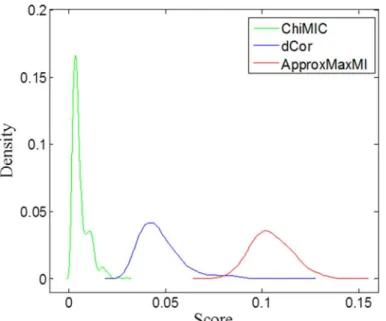
For the null hypothesis of statistical independency, a larger average value and standard devi-ation for the dependency measure indicate lower statistical power. Therefore, for two indepen-dent variables, a good dependency measure should have small standard deviation and zero average value, although small average value and standard deviation do not directly mean high statistical power.Fig 7illustrates the density distribution of MIC values calculated by Approx-MaxMI and ChiMIC, as well as the dCor scores for the null hypothesis. Obviously, MIC values calculated by ChiMIC have a smaller average value and standard deviation. Therefore, they potentially have higher statistical power.
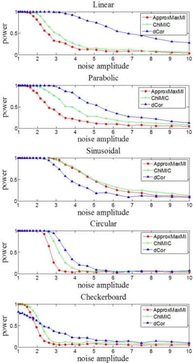
However, the statistical power of dependency measures may depend on different factors, such as pattern types, noise levels and sample sizes. We examine the statistical power of dCor and MIC calculated by ApproxMaxMI and ChiMIC for five different functions with different noise levels. As shown inFig 8, the statistical powers of MIC calculated by ChiMIC are higher than those of MIC calculated by ApproxMaxMI for all five functional relationships. For linear, parabolic and circular functional relationships, dCor has higher statistical power than those of MIC calculated by ApproxMaxMI and ChiMIC. For sinusoidal function, statistical power of MIC calculated by ApproxMaxMI and ChiMIC are both higher than that of dCor. For checker-board function, MIC calculated by ApproxMaxMI and ChiMIC outperform dCor at low noise levels, while dCor outperforms at high noise levels.
Comparison of computational cost of ApproxMaxMI and ChiMIC
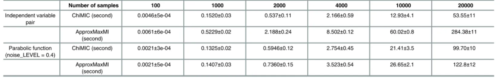
compare the computational time of ChiMIC and ApproxMaxMI using different sizes of inde-pendent variable pairs. As shown inTable 1, the run times of ChiMIC algorithm are signifi-cantly less than those of ApproxMaxMI algorithm. This is because ChiMIC algorithm uses the chi-square test to terminate grid optimization earlier, while ApproxMaxMI algorithm always tends to search to the maximal grid size B(n). When sample size is 100, ChiMIC algorithm is about 30% faster than ApproxMaxMI algorithm. As samples sizes increase, the advantage of Fig 8. Statistical power of MIC from ApproxMaxMI, ChiMIC and dCor with different levels of noise, for five kinds of functional relationships.The statistical power was estimated via 500 simulations, with sample sizen= 400.
doi:10.1371/journal.pone.0157567.g008
ChiMIC algorithm becomes even more evident. When the sample size is 20000, ChiMIC algo-rithm runs nearly five times faster than ApproxMaxMI algoalgo-rithm does. For the parabolic func-tion with noise_LEVEL is 0.4, ChiMIC algorithm also has a faster convergence speed. Thus, ChiMIC algorithm will be a better method for calculating MIC values of big data.
Application of MIC values to selecting features for cancer classification
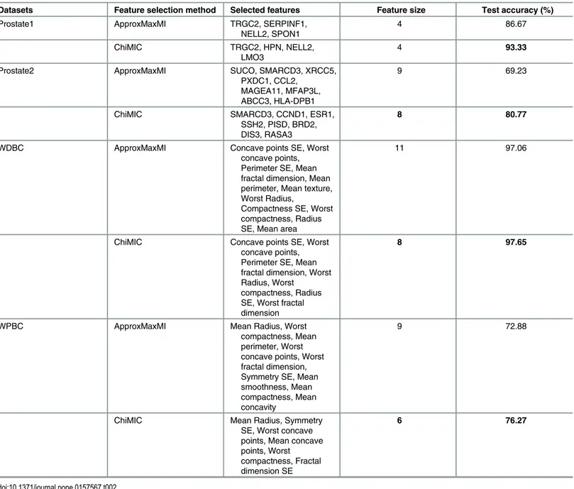
The dependency measures can be used to select features. We compare the MIC values calcu-lated by ApproxMaxMI and ChiMIC in feature selection. We test feature selection on four can-cer classification data sets: two microarray datasets (Prostate1 and Prostate2) and two image datasets (WDBC and WPBC). We partition each dataset into a training set and a test set ran-domly (see details in theMethodsection). The training set is used for feature selection and clas-sifier construction, and the test set is used for model validation. The retained features and independent test accuracies for the four datasets are shown inTable 2. For the Prostate1 data-set, although the methods based on MIC values from ApproxMaxMI and ChiMIC both select four features, features selected by MIC values from ChiMIC give much higher test accuracy (93.33% vs. 86.67%). For the other three data sets, MIC values from ChiMIC select fewer fea-tures than those selected by MIC values from ApproxMaxMI. All classifiers based on feafea-tures selected by MIC values from ChiMIC obtain higher test accuracy. Especially for the Prostate2 dataset, the test accuracy of classifier based on features selected by MIC values from ChiMIC (80.77) is 11.54% higher than that of classifier based on features selected by MIC values from ApproxMaxMI (69.23%). This result suggests that the features selected by MIC values from ChiMIC are more effective.
Methods
ChiMIC algorithm: determining optimal grid using chi-square test
Same as ApproxMaxMI [9] algorithm, the ChiMIC algorithm partitions a data set of ordered pairs throughx-axis andy-axis. Similar to ApproxMaxMI [9] algorithm, the ChiMIC algo-rithm tries to find optimal partition ofx-axis given an equipartition ofrbins ony-axis. For example, inFig 9A, the first optimal endpoint EP1dividesx-axis into two bins. Then, we will use a chi-square test to determine whether the next endpoint is useful. If thep-value of chi-square test is lower than a given threshold, the endpoint is useful and the ChiMIC algorithm continues searching for next optimal endpoint. On the other hand, if thep-value of chi-square test is greater than the given threshold, the endpoint is not useful and the process of partition x-axis is terminated.
Table 1. Elapsed time for calculating MICs for different sample sizes.
Number of samples 100 1000 2000 4000 10000 20000
Independent variable pair
ChiMIC (second) 0.0046±5e-04 0.1520±0.03 0.537±0.11 2.166±0.59 12.93±4.1 53.55±11
ApproxMaxMI (second)
0.0061±6e-04 0.5229±0.02 2.188±0.24 8.502±0.12 60.02±0.8 284.38±11
Parabolic function (noise_LEVEL = 0.4)
ChiMIC (second) 0.0021±3e-04 0.1325±0.02 0.5946±0.12 2.754±0.45 21.41±3.5 99.70±10
ApproxMaxMI (second)
0.0021±5e-04 0.1407±0.03 0.7360±0.15 3.523±0.54 26.65±2.1 122.8±12
The corresponding time was represented as the average value±standard deviation over 100 time replicated runs on a Windows 7 32-bit operating
The chi-square statistic is defined in Eq (3):
w2 EPm ¼
Xr
i¼1
Xkþ1
j¼k
ðfij niTj=NÞ 2
niTj=N
ð3Þ
where themth(m>1) new endpoint EPmdividesx-axis into thekthand(k+1)thbin.i
(i= 1,2,. . .,r) denotes theithbin ofy-axis,j(j=k,k+1) denotes thejthbin ofx-axis.fijdenotes the number of sample points falling into the cell in theithrow andjthcolumn.nidenotes the
number of sample points falling in theithrow,Tjdenotes the number of sample points falling
in thejthcolumn,Ndenotes the total number of sample points falling in thekthand(k+1)th col-umns. For example, inFig 9B, the second optimal endpoint EP2is selected by dynamic
Table 2. Retained features and independent test accuracy based on MIC and ChiMIC.
Datasets Feature selection method Selected features Feature size Test accuracy (%)
Prostate1 ApproxMaxMI TRGC2, SERPINF1,
NELL2, SPON1
4 86.67
ChiMIC TRGC2, HPN, NELL2,
LMO3
4 93.33
Prostate2 ApproxMaxMI SUCO, SMARCD3, XRCC5,
PXDC1, CCL2, MAGEA11, MFAP3L, ABCC3, HLA-DPB1
9 69.23
ChiMIC SMARCD3, CCND1, ESR1,
SSH2, PISD, BRD2, DIS3, RASA3
8 80.77
WDBC ApproxMaxMI Concave points SE, Worst
concave points, Perimeter SE, Mean fractal dimension, Mean perimeter, Mean texture, Worst Radius,
Compactness SE, Worst compactness, Radius SE, Mean area
11 97.06
ChiMIC Concave points SE, Worst
concave points, Perimeter SE, Mean fractal dimension, Worst Radius, Worst
compactness, Radius SE, Worst fractal dimension
8 97.65
WPBC ApproxMaxMI Mean Radius, Worst
compactness, Mean perimeter, Worst concave points, Worst fractal dimension, Symmetry SE, Mean smoothness, Mean compactness, Mean concavity
9 72.88
ChiMIC Mean Radius, Symmetry
SE, Worst concave points, Mean concave points, Worst compactness, Fractal dimension SE
6 76.27
doi:10.1371/journal.pone.0157567.t002
programming. The sample points distributed in the blue area (thex2thcolumn andx3thcolumn inFig 9B) are used to perform a chi-square test on anr×2 contingency table. If EP2is useful, then ChiMIC continues searching for the next optimal endpoint. If the next one is EP3, we use the sample points distributed in the green area to perform a chi-square test on anr×2 contin-gency table (Fig 9C). Ifp-value is greater than the given threshold, the optimizing process is ter-minated. For the chi-square test, the minimum expected count in each group isfive [28]. The p-value of chi-square test for a 2×2 table with data counts {0, 5; 5, 0} is 0.0114. So we choose 0.01 as the threshold. The Chi-square value needs correction for continuity whenr= 2 [29].
Adding noise to functional relationship
The noise to functional relationships inS1 Fig,Fig 2,Fig 3,Fig 4andFig 6are defined as fol-lows:
Y¼fðXÞ þ ðRANDðN;1Þ 0:5Þ noise LEVELRANGE ð4Þ
wherefis a functional relationship, and RANGE represents the range off(X). noise_LEVEL is the relative amplitudes: 0, 0.2, 0.4, 0.6, 0.8, 1.0, 1.2,1.4, 1.6, 1.8, 2.0. RAND(N, 1) is used to gen-erateNrandom numbers in [0, 1].
The noise functional relationships inFig 8are defined inTable 3. Five hundred trial datasets are generated for each of these relationships at each of twenty-five different noise amplitudes (a) distributed logarithmically between 1 and 10. For each dataset, statistics are computed on the“true”data {Xi,Yi}(i= 1,. . .,400) as well as on“null”data, for which the indicesion they
values are randomly permuted. The power of each statistic is defined as the fraction of true datasets yielding a statistic value greater than 95% of the values yielded by the corresponding Fig 9. Illustration of x-axis partition of ChiMIC.Coloredr×2 contingency tables are used for chi-square test. doi:10.1371/journal.pone.0157567.g009
Table 3. TheX,Yrelationships simulated for the power calculations inFig 8.
Relationship X Y
Linear ξ 2/3X+aη
Parabolic ξ X2 +aη
Sinusoidal 5/2θ 2 cos(X) +aη
Circular 10 cos(θ) +aξ 10 sin(θ) +aξ
Checkerboard 10X0+aξ 10Y0+aη
null datasets.ξandηare random numbers drawn from the normal distributionN(0,1).θis a
random number drawn uniformly from the interval [−π,π). (X0,Y0) is a pair of random
num-bers drawn uniformly from the solid squares of a 4×5 checkerboard, where each square has sides of length 1[26].
Real datasets
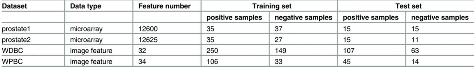
We use four real datasets to validate the proposed approach. Prostate1 [30] and Prostate2 [31] are gene expression profile datasets. Wisconsin Diagnostic Breast Cancer (WDBC) and Wis-consin Prognostic Breast Cancer (WPBC) [32] are image data of tumor tissues obtained from UCI database, which can be download athttp://archive.ics.uci.edu/ml/data. The number of fea-tures, positive and negative samples in both training set and test set are listed inTable 4.
Feature selection
For each dataset, first, we calculate MIC values of a vector (X,Y) separately in training set, whereXdenotes the value of each feature, andYdenotes the phenotype of tumors. Then, we rank all the features in descending order of MIC values. Next, we sequentially introduce the ranked features (only top 200 features for datasets Prostate1 and Prostate2) and remove redun-dant features using 10-fold cross-validation based on support vector classification (SVC). Finally, we build a SVC prediction model based on retained features using training data and perform independent prediction on test data.
Computational Methods
The ChiMIC (S1 File) and ApproxMaxMI algorithms are both implemented in Matlab. The parameters of ApproxMaxMI are set asa= 0.6,c= 5. dCor and statistical power are computed using Matlab scriptsdownloaded athttp://www.sourceforge.net[26]. The SVC is performed using LIBSVM [33] described by Changet al, and can be downloaded athttp://www.csie.ntu. edu.tw/~cjlin/libsvm/index.html.
Supporting Information
S1 Fig. 21 Noiseless functions.(DOCX)
S1 File. This is the ChiMICMatlab code. (ZIP)
S1 Table. 21 Functional relationships.
(DOCX)
S2 Table. MIC values of each functional relationship with noise.
(DOCX)
Table 4. Datasets: Training set and test set are divided randomly at a ratio of 7:3.
Dataset Data type Feature number Training set Test set
positive samples negative samples positive samples negative samples
prostate1 microarray 12600 35 37 15 15
prostate2 microarray 12625 35 27 15 11
WDBC image feature 32 250 149 107 63
WPBC image feature 34 106 33 45 14
doi:10.1371/journal.pone.0157567.t004
Author Contributions
Conceived and designed the experiments: YC ZMY. Performed the experiments: YC YZ. Ana-lyzed the data: YC FL ZMY. Contributed reagents/materials/analysis tools: YC YZ. Wrote the paper: YC YZ FL ZMY. Designed the software used in analysis: YC YZ.
References
1. Hanson B, Sugden A, Alberts B. Making data maximally available. Science. 2011; 331: 649–649. doi: 10.1126/science.1203354PMID:21310971
2. Pearson K. Notes on the history of correlation. Biometrika. 1920; 13: 25–45. 3. Kendall MG. A new measure of rank correlation. Biometika. 1938; 30: 81–93.
4. Moon YI, Rajagopalan B, Lall U. Estimation of mutual information using kernel density estimators. Phys Rev E. 1995; 5: 2318–2321.
5. Kraskov A, Stogbauer H, Grassberger P. Estimating mutual information. Phys Rev E. 2004; 69: 066138.
6. Walters-Williams J. Estimation of mutual information: A survey. Lect Notes Comput Sc. 2009; 5589: 389–396.
7. Szekely GJ, Rizzo M, Bakirov NK. Measuring and testing independence by correlation distance. Ann Stat.2007; 35: 2769–2794.
8. Delicado P, Smrekar M. Measuring non-linear dependence for two random variables distributed along a curve. Stat Comput. 2009; 19: 255–269.
9. Reshef DN, Reshef YA, Finucane HK, Grossman SR, McVean G, Turnbaugh PJ, et al. Detecting Novel Associations in Large Data Sets. Science. 2011; 334: 1518–1524. doi:10.1126/science.1205438 PMID:22174245
10. Zhang Y, Jia S, Huang H, Qiu J, Zhou C. A Novel Algorithm for the Precise Calculation of the Maximal Information Coefficient. Sci Rep-Uk. 2014; 4: 6662.
11. Speed T. A correlation for the 21st century. Science.2011; 334: 1502–1503. doi:10.1126/science. 1215894PMID:22174235
12. Lin C, Miller T, Dligach D, Plenge RM, Karlson EW, Savova G. Maximal information coefficient for fea-ture selection for clinical document classification. ICML Workshop on Machine Learning for Clinical Data. Edingburgh, UK. 2012.
13. Das J, Mohammed J, Yu H. Genome-scale analysis of interaction dynamics reveals organization of bio-logical networks. Bioinformatics. 2012; 28: 1873–1878. doi:10.1093/bioinformatics/bts283PMID: 22576179
14. Anderson TK, Laegreid WW, Cerutti F, Osorio FA, Nelson EA, Christopher-Hennings J, et al. Ranking viruses: measures of positional importance within networks define core viruses for rational polyvalent vaccine development. Bioinformatics. 2012; 28: 1624–1632. doi:10.1093/bioinformatics/bts181PMID: 22495748
15. Song L, Langfelder P, Horvath S. Comparison of co-expression measures: mutual information, correla-tion, and model based indices. BMC bioinformatics. 2012; 13: 328. doi:10.1186/1471-2105-13-328 PMID:23217028
16. Riccadonna S, Jurman G, Visintainer R, Filosi M, Furlanello C. DTW-MIC coexpression networks from time-course data. arXiv preprint arXiv: 1210.3149, 2012.
17. Moonesinghe R, Fleming E, Truman BI, Dean HD. Linear and non-linear associations of gonorrhea diagnosis rates with social determinants of health. Inter J Env Res Pub Heal. 2012; 9: 3149–3165. 18. Lee SC, Pang NN, Tzeng WJ. Resolution dependence of the maximal information coefficient for
noise-less relationship. Stat Comput. 2014; 24: 845–852.
19. de Souza RS, Maio U, Biffi V, Ciardi B. Robust PCA and MIC statistics of baryons in early minihaloes. Mon Not R Astron Soc. 2014; 440: 240–248.
20. Zhang Z, Sun S, Yi M, Wu X, Ding Y. MIC as an Appropriate Method to Construct the Brain Functional Network. Biomed Res Int. 2015; 2015: 825136. doi:10.1155/2015/825136PMID:25710031
21. Tang D, Wang M, Zheng W, Wang H. RapidMic: Rapid Computation of the Maximal Information Coeffi-cient. Evol Bioinformatics Online. 2014; 10: 11.
23. Albanese D, Filosi M, Visintainer R, Riccadonna S, Jurman G, Furlanello C. minerva and minepy: a C engine for the MINE suite and its R, Python and MATLAB wrappers. Bioinformatics. 2013; 29: 407–
408. doi:10.1093/bioinformatics/bts707PMID:23242262
24. Reshef DN, Reshef YA, Finucane HK, Grossman SR, McVean G, Turnbaugh PJ, et al. Supporting Online Material for Detecting Novel Associations in Large Data Sets. Science. 2011; 334: 1518–1524. doi:10.1126/science.1205438PMID:22174245
25. Gorfine M, Heller R, Heller Y. Comment on“Detecting Novel Associations in Large Data Sets”[EB/OL]. 2014. Available:http://www.math.tau.ac.il/~ruheller/Papers/science6.pdf.
26. Kinney JB, Atwal GS. Equitability, mutual information, and the maximal information coefficient. Proc. Natl Acad. Sci. USA. 2014; 111: 3354–3359. doi:10.1073/pnas.1309933111PMID:24550517 27. Simon N, Tibshirani R. Comment on‘Detecting novel associations in large data sets’by Reshef et al,
Science Dec 16, 2011. arXiv preprint arXiv:1401, 7645. 2014. Available:http://statweb.stanford.edu/~ tibs/reshef/comment.pdf.
28. Cochran WG. Sampling Techniques. 2st ed. New York: John Wiley & Sons; 1963.
29. Yates F. Contingency tables involving small numbers and theχ2 test. J Roy Stat Soc. 1934; Suppl.1: :
217–235.
30. Singh D, Febbo PG, Ross K, Jackson DG, Manola J, Ladd C, et al. Gene expression correlates of clini-cal prostate cancer behavior. Cancer Cell. 2002; 2: 203–209.
31. Stuart RO, Wachsman W, Berry CC, Wang-Rodriguez J, Wasserman L, Klacansky I, et al. Stuart In sil-ico dissection of cell-type-associated patterns of gene expression in prostate cancer. Proc. Natl Acad Sci USA. 2004; 101: 615–620. PMID:14722351
32. Blake CL, Merz CJ. UCI repository of machine learning databases. Available:http://www.ics.uci.edu/~ mlearn/mlrepository.html. University of California, Irvine, Dept. of Information and Computer Sciences, 1998.