Comparison between resistant load contours
generated considering the parabolic-rectangular
(DPR) and the rectangular (DR) stress-strain diagrams
for rectangular sections under combined axial
compression and biaxial bending
Comparação entre envoltórias de esforços resistentes
geradas considerando os diagramas parábola
retângulo (DPR) e retangular (DR) de
tensão-deformação no concreto para seções retangulares
solicitadas à flexo-compressão oblíqua
a Universidade Federal da Bahia, Escola Politécnica, Departamento de Construção e Estruturas, Salvador, BA, Brasil.
Received: 12 Feb 2017 • Accepted: 29 Aug 2017 • Available Online:
Y. F. FONSECA a
yasminfortes@gmail.com
A. S. C. SILVA a
aloisiosthefano@gmail.com
Abstract
Resumo
The aim of this study is to compare the load contour diagrams generated for rectangular RC cross-sections under combined axial compression and
biaxial bending obtained by the two forms of analysis allowed by NBR 6118:2014 [1]: the first using the parabolic-rectangular stress-strain diagram
(DPR) and the second using the rectangular (constant stress) diagram (DR). In order to compare the load contours generated, a reference cross-section was adopted for which the concrete strength class (from C20 to C90) and the deformation domains (4, 4a and 5) were varied for the study.
It was studied whether the use of the different diagrams (DPR or DR) would provide greater (or smaller) resistant efforts for the same section. The
results show that the use of the DR is only acceptable when the section is working up to the 4th domain. Above this domain, it was observed that
the use of this diagram shows resistant efforts inferior to those calculated by the DPR. In addition, it was found that, for concretes with resistance class above C50, in oblique loading directions, the use of the DR presents higher resistant efforts than those calculated using the DPR.
Keywords: combined compression and biaxial bending, load contours, resistance assessment, reinforced concrete.
Esse trabalho tem o objetivo de comparar as envoltórias de resistência geradas para seções transversais retangulares de concreto armado
solicitadas à flexo-compressão oblíqua a partir das duas formas de análise permitidas pela NBR 6118:2014 [1]: a primeira utilizando o diagrama tensão-deformação parábola-retângulo do concreto (DPR) e a segunda utilizando o diagrama retangular (simplificado) de tensões no concreto (DR). Para comparar as envoltórias geradas, adotou-se uma seção transversal de referência, onde variou-se a classe de resistência do concreto (de C20 a C90) e o domínio de deformação da peça (entre os domínios 4, 4a e 5) para o estudo. Foi aferido sobre qual diagrama (DPR ou DR) apresenta esforços resistentes maiores (ou menores) para uma mesma seção. Os resultados encontrados mostram que o uso do DR só se justifica quando a peça tiver trabalhando até o domínio 4. Acima desse domínio, foi observado que o uso desse diagrama apresenta esforços re
-sistentes inferiores aos calculados pelo DPR. Além disso, verificou-se que, para concretos com classe de resistência acima de C50, em direções oblíquas de solicitação, o uso do DR apresenta maiores esforços resistentes do que os calculados utilizando o DPR.
1. Introduction
In order to ensure the safety of a reinforced concrete element, while respecting its ultimate limit state (ELU), this element must resist any possible loads that may occur during its service life. Particularly for a compressed section, when bending loads can be neglected or when it is possible to ensure that bending is about one of the main inertia
directions, verification can be done in a simpler way, either from sim -ple axial compression analysis or combined axial compression and uniaxial bending, respectively. However, in general, the structural el-ements are subjected to loading combinations that might have their
maximum effects ocurring obliquely to the main directions of inertia.
In such cases, it is necessary that the analysis is performed consid-ering combined axial compression and biaxial bending.
The combined axial compression and biaxial bending analysis is performed with the generation of a capacity surface for the element cross-section (Figure 1), in which, for each axial compression load,
the resisting moments are obtained about the different load direc -tions (from 0° to 360°). To assure section security, any combination of applied loads (axial compression and bending moments) must be contained within the capacity surface obtained.
To simplify the comparison between section capacity and applied loads, it can be presumed that the design axial load strength (NRd) must be equal to the factored applied axial load (Nsd) obtained for the structure. Thus, the analysis is limited to the curve representing the load contour of the section for the given axial load (see Figure 2). The total cross-section strength is composed by the contribution portion of each rebar added to the contribution portion of the com-pressed concrete area. NBR 6118:2014 [1] allows the concrete
contribution to be defined in two ways. The first, using the parabol -ic-rectangular stress-strain diagram, as described in item 8.2.19.1
of [1], and the second using the rectangular (simplified) diagram,
according to item 17.2.2 of [1].
According to the Fib MC2010 [2] standard, the parabolic-rectangular diagram is the one that best describes the stress distribution in the
compressed zone of the concrete for sections subjected to com -bined axial compression and biaxial bending, in fact, many other normative standards allow the use of this diagram such as the NBR 6118: 2014 [1] and the EN 1992-1-1: 2004 [3]. Hence, the use of the rectangular diagram is a process of analytical approximation allowed by NBR 6118: 2014 [1] (also allowed by other standards)
that is justified by the mathematical simplification that it offers in the
evaluation of the strength capacity of reinforced concrete sections. The aim of this study is to compare the load contours obtained for rectangular reinforced concrete sections subjected to combined axial compression and biaxial bending generated from the two forms of analysis mentioned above and to verify in which situations
the use of the simplified diagram can contribute to uneconomical or unsafe design. In this comparison, the influences of the strain
domain variation (domains 3, 4, 4a and 5) and of the concrete strength class variation (C20 to C90) were observed.
2. Load contour generation
2.1 Equilibrium equations
For combined axial compression andbendingabout oblique direc-tions, the neutral axis (N.A.) slope is not necessarily perpendicular to the plane of action of the bending moment (MSd), unlike what happens for uniaxial bending (Santos [4]). Thus, both the slope (α) of the N.A. and its depth (X) relative to the most compressed
con-crete fiber represent unknowns for design, which makes it consid -erably more complex (Figure 3). According to (Campos [5]), these two parameters (α and X) define the strain state of the section.
Each load contour can then be generated from the calculation of the moment strength about the two main inertia directions (x,y) for
α values varying from 0° to 360°. For each value of α considered, the depth of the N.A must be calculated such that the resulting axial strength load equals the applied axial load. For calculation
Figure 1
Capacity surface between axial and moment
strengths
Figure 2
purposes, it is convenient to define a new cartesian plane that fol -lows the strain orientation in the section (Campos [5]). Hence, the initial cartesian plane of the section (x,y) is rotated by the angle
αto establish the new plane (ξ,η), in which the abscissa axis (ξ) is located parallel to the N.A. and the ordinate axis (η) points towards
the most compressed fiber. The vertices and bars coordinates that define the section must be transformed from the initial cartesian
plane (x,y) to the rotated plane (ξ,η), through the equations (1) and (2) bellow:
(1)
(2)
In this work, the sign convention adopted is positive for axial com-pression load and bending moments should be considered positive as indicated in Figure 4.
For a known strain state (α and X) and from the concrete and steel stresses, three equilibrium equations can be obtained, as expressed in equations (3), (4) and (5). These equations are used to establish the design moment strengths for each angle of N.A. slope.
(3)
(4)
(5)
where:
NRd = design axial load strength
MRηd = design moment strength about η axis
MRξd = design moment strength about ξ axis
n = total number of rebars; σc = stress on concrete;
σs = stress on steel; Abj = steel area of rebar j; Acc = concrete compressed area; εj = strain in rebar j;
εc = strain in concrete.
The axial load is independent of the reference cartesian plane. However, the moment strengths (about ξ and η axis) must be
transformed back into the initial cartesian plane (x,y) so that they can be compared with the applied moments. This can be done from equations (6) e (7) bellow:
(6)
(7)
From the set of moment strengths obtained for the various val-ues of α, the load contour that represents the section capacity
can be generated. For economical design, the difference be -tween applied bending moments and the lload contour limits
must not be significant.
2.2 Strain calculation
After defining the strain domain of the section, it is possible to calcu -late the strain at the ends of the section (εs and εi) and to establish a relation between them that allows the calculation of the strain for
ev-ery section point. Thereby, it is possible to define the strain of each rebar present in the analyzed reinforced concrete section.
Following the procedure adopted by (Campos [5]), from the maxi-mum (ηv,máx) and minimum (ηv,min) vertices ordinates and the mini-mum rebar ordinate (ηs,mín), that is, the ordinate of the most ten-sioned rebar, both the height (h = ηv,máx - ηv,mín) and the effective
depth of the section (d = ηv,máx - ηs,mín) can be defined, as shown in
Figure 5.
The relation between strains, expressed by the equation (8), can be used to calculate the strain at a generic point in the section with ordinate ηj.
(8)
to simplify this equation, it can be rewritten as:
(9)
Figure 3
Strain state defined for a given depth and slope
of N.A.
Figure 4
Where b is the section curvature, given by equation (10), and c is
the strain of the fiber located at the center of gravity of the section,
calculated by equation (11).
(10)
(11)
2.3 Calculation of steel strength
To define compression and bending steel strength, each rebar
is considered to contribute independently to the section total strength. In this way, the total strength calculation is taken as the
sum of the strength offered by each rebar. The strain in each rebar is defined as a function of its ordinate and depends on the strain
domain of the section. With that, the respective steel stresses (σs) are calculated considering the stress-strain diagram of the material
(item 8.3.6 of NBR 6118:2014 [1]). Finally, the total strength offered
by steel is calculated as expressed in equations (3), (4) and (5).
2.4 Calculation of concrete strength
For concrete strength calculation, NBR 6118:2014 [1] defines the
parabolic-rectangular stress-strain diagram for classes C20 to C90 as shown in Figure 6.
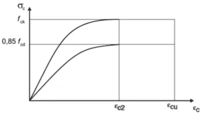
Overall, these diagrams present a curved initial part, which extends until the strain equals εc2 (specific shortening strain of concrete at
reaching the maximum strength) and is followed by a constant part until it reaches the strain εcu (specific shortening strain of concrete at ultimate strength), as shown in Figure 7.
The equation that defines stress in the curved part of the diagram
is given by:
(12)
where, fcd = fck/1,4
fck = characteristic compressive strength of concrete specimens tested at 28 days
fcd = design compressive strength of concrete
As defined in item 8.2.10.1 of NBR 6118:2014 [1], the index value n depends on the fck and is given as n = 2, for fck ≤ 50MPa, and as n = 1,4 + 23,4 [(90 - fck)/100]4, for 50MPa < f
ck < 90MPa.
In order to ease the calculation of concrete strength for fck > 50MPa,
it is proposed by (Campos [5]) that the first part of the diagram is
approximated to a parabola of the second degree passing through
the origin. This author defines this parabola equation as:
(13)
where a1 and a2 are the coefficients that correlate the real curve and the approximated parabola.
Figure 5
Height and effective depth
Figure 6
By adjusting parabolas to stress-strain curves performed with Mi-crosoft Excel software, the values for a1 and a2 shown in Table 1 are obtained.
It was observed that the correlation coefficients (R²) between the
actual curves and the parabolic approximations had values very
close to 1 (around 0,998), which confirms that the adoption of
parabolic curves to represent the material behavior is satisfactory. As stated in item 17.2.2 of NBR 6118:2014 [1], in addition to the
parabolic-rectangular diagram of stresses for concrete, a simplified
rectangular diagram with height y = λX can be used (see Figure 8). In this diagram, acting stress is considered constant up to the depth y and is equal to αc.fcd when the section width (measured parallel to the N.A.) does not decrease therefrom to the compressed edge. For combined axial compression and biaxial bending, this occurs for N.A. with slopes α = (0°,90°,180°,270°,360°). For other slopes,
the section width decreases towards the most compressed fiber
and, in such cases, the constant stress of the diagram must be considered equal to 0,9.αc.fcd. As recommended by (Santos [4]), it is convenient that this reduced stress is used regardless of the slope of the neutral axis. The parameters λ and αc are defined
as functions of the compressive strength of the concrete, accord-ing to item 17.2.2 of NBR 6118:2014 [1], as 0,8 and 0,85, respec-tively, for fck ≤ 50MPa and through equations (14) and (15) for 50MPa < fck < 90MPa.
(14)
(15)
The concrete contribution to strength is obtained from integrations over the compressed concrete area of the section as described in equilibrium equations (3), (4) e (5), where the stress in concrete is obtained through the strain calculated for each ordinate. To solve
these integrals, different procedures can be adopted. Works like the ones of (Campos [5]) and (Muniz [6]) use the Green Theorem
to transform surface integrals into contour integrals that are solved along the vertices of the compressed section area. Other works
such as those of (Cardoso Júnior [7]) and (Suaznábar e Silva [8]) use the cross-section discretization to solve the same problem
analytically. This work has adopted the methodology detailed in (Campos [5]) for load contour generation.
3. Comparative analysis of load contours
In order to evaluate the differences between the load contours gen -erated using the parabolic-rectangular or the rectangular diagrams, a case study was carried out for a reference cross-section (Figure 9). For this, a program was implemented in Microsoft Excel software based on the concepts presented previously. The program enables the generation of load contours by both methods. The program
pre-sentation is better defined in the work of (Fonseca [9]).
Figure 10 presents an example of load contour overlapping gener-ated by the program considering the C30 strength concrete class
Table 1
a
1and a
2correlation coefficients between actual stress-strain curve and the approximated parabola
fck (MPa) ≤ 50 60 70 80 90
a1 1 0,72055 0,62031 0,58129 0,56158
a2 -0,25 -0,12564 -0,08679 -0,07422 -0,06927
Figure 7
Stress-strain diagram for concrete (source: [1])
Figure 8
Rectangular concrete stresses diagram (simplified)
Figure 9
and the 950 KN axial load strength. In addition to graphic result, the program also provides the moment strength of the section for each slope of the assumed neutral axis (from 0º to 360º), every 5°, in a table.
Initially, as a means to investigate the differences between axial
strengths obtained by the parabolic-rectangular and rectangular diagrams for sections under pure axial compression, the value of the maximum axial load design strength of the model section in
domain 5 was verified. For this, it was considered N.A. tending to infinity and fully compressed section with constant strain εc2. Table 2 lists the values obtained for the maximum axial load design strength considering the parabolic-rectangular and rectangular diagrams for concrete strength classes C20 to C90.
It can be observed that for concretes with fck ≤ 50MPa the dif -ference between the axial load strengths is not very expressive, reaching the maximum of 8%. However, for higher strength
classes, the difference increases as the fck becomes higher, reaching 24% for C90 concretes. In building structures, it is usual to adopt concretes with fck ≤ 50MPa, nevertheless, for
cases where the fck used is superior, the design done using the rectangular diagram can become uneconomical, since there could be considered a higher axial load strength calculated by the parabolic-rectangular diagram.
In addition, this work also sought to evaluate how the differences between load contours are influenced by the increase in the strain
domain and by the variation on the concrete strength class. Table 3 presents the results found for moment strengths corresponding to N.A. slopes of 0°, 45° and 90°, using concretes with strength classes C20 to C90 and increasing values for the factored applied axial load.
For all strength classes, the depth of the N.A grows with the in-crease of the axial load, as there must be a larger compressed concrete area for section equilibrium. Consequently, the strain do-main also increases. Evaluating the results of Table 3, it can be ob-served that the higher the strain domain becomes, the greater are
the differences between moment strengths (independently of the N.A. slope). In domain 4, these differences are moderate, reaching
the maximum of 15%, whereas in domain 4a, and especially in
do-Figure 10
Example of load contour overlapping
Table 2
Comparison between maximum axial load design strengths
fck (MPa) NRd (KN) calculated through the use of: variationPercent
DPR DR
20 2058,7 1937,3 6%
30 2665,9 2483,7 7%
40 3273,0 3030,2 7%
50 3880,2 3576,6 8%
60 4490,8 3988,8 11%
70 5093,3 4316,7 15%
80 5696,5 4589,9 19%
90 6294,5 4808,5 24%
angular diagram, so that the design done with the rectangular diagram is always in safety favor for such cases. Nonetheless, for fck > 50MPa and strain domains 3 and 4, it can be noticed that the oblique moment strength obtained by the rectangular diagram becomes larger than that obtained by the parabolic-rectangular
diagram, as exemplified in Figure 12. This situation presents the possibility of realizing an unsafe design when adopting the rect -angular diagram. It is observed that for strength classes C70 and
As shown in Table 2, the percent variation between the axial load strengths obtained increased with the increase in fck, especially for
concretes above C50 class. This is justified because, for a fully
compressed section, all concrete area is resisting under a stress of 0,85fcd when using the parabolic-rectangular diagram, which is greater than the assumed 0,9αc fcd stress when using the rectangu-lar diagram. For values of fck ≤ 50MPa, the αc value is equal to 0,85, but, according to equation (15), this value decreases with increasing
Figure 11
Load contour overlapping for an example section on domain 5
Figure 12
fck, so that the stress calculated with the simplified diagram becomes more conservative with increasing concrete strength classes. Similarly, as presented in Table 3, for sections between the do-mains 4a and 5, the percent variation between moment strengths obtained is very expressive and becomes larger with the increase in the strain domain. For these predominantly compressed
sec-tions, the stress acting over the entire cross-section according to the parabolic-rectangular diagram becomes close to its peak stress (0,85fcd) and, for this reason, the consideration of an in-ferior constant compressive stress for the rectangular diagram
(0,9αc fcd) impacts on the decrease of moment strengths calculated using this diagram.
Table 3
Comparison between moment strengths
fck
(MPa) Nsd Domain
MRd,α= 0° (KN.m)
calculated by: Perc.
Var.
MRd,α= 45° (KN.m)
calculated by: Perc.
Var.
MRd,α= 90° (KN.m)
calculated by: Perc.
Var.
DPR DR DPR DR DPR DR
20
70 4 168,9 159,1 6% 143,7 137,6 4% 73,5 68,9 6%
110 4 140 128,6 8% 123,6 116,1 6% 58,0 53 9%
150 4a 95,2 81,9 14% 84,6 74,0 13% 38,1 32,3 15%
190 5 29,8 9,6 68% 28,1 8,6 69% 11,9 4 66%
30
95 4 206,8 193,9 6% 178,3 170,0 5% 89,2 82,8 7%
145 4 176,1 159,8 9% 156,4 145,8 7% 72,5 65,5 10%
195 4a 122,1 101,8 17% 108,7 92,4 15% 48,9 40,3 18%
245 5 39,7 9 77% 37,6 8,1 78% 15,8 3,8 76%
40
120 4 243,7 228,6 6% 212,6 202,4 5% 104,6 96,6 8%
180 4 212 191 10% 189,3 175,6 7% 86,9 78 10%
240 4a 148,9 121,6 18% 132,7 110,8 17% 59,6 48,2 19%
300 5 49,8 8,5 83% 47,2 7,5 84% 19,7 3,6 82%
50
145 4 280,5 263,1 6% 246,8 234,7 5% 119,8 110,4 8%
215 4 247,9 222,4 10% 222,1 205,4 8% 101,3 90,5 11%
285 4a 175,7 141,5 19% 156,8 129,2 18% 70,4 56,2 20%
355 5 59,9 7,9 87% 56,8 7,0 88% 23,7 3,4 86%
60
170 4 286,5 273 5% 238,6 244,9 -3% 118,7 113,5 4%
245 4 253,8 233,3 8% 211,2 213,9 -1% 105,2 96,8 8%
320 4a 177,8 145,6 18% 149,2 130,0 13% 72,4 59,4 18%
395 5 74,2 6,8 91% 62,0 6,1 90% 29,9 2,3 92%
70
190 4 298,8 286,9 4% 242,3 258,8 -7% 122,1 117,4 4%
270 4 265,3 245,5 7% 209,4 224,8 -7% 109,7 102 7%
350 4a 184,6 148,7 19% 144,5 131,1 9% 76,2 62,1 18%
430 5 91,4 3,2 97% 71,3 3,1 96% 36,9 1 97%
80
200 4 321,3 302 6% 258,6 272,8 -6% 130,7 123,1 6%
285 4 291,4 262,1 10% 227,3 240,8 -6% 119,6 108,2 10%
370 4a 212,6 162,7 23% 162,8 143,8 12% 87,8 67,8 23%
455 5 118,9 3,8 97% 91,0 3,7 96% 48,0 1,2 98%
90
210 4 346,5 313,4 10% 278,8 283,8 -2% 140,6 127,6 9%
300 4 320,5 273,4 15% 250,5 252,0 -1% 131,1 112,7 14%
390 4a 243,3 168,6 31% 185,4 149,5 19% 100,3 69,8 30%
480 5 150,3 1,8 99% 114,6 1,7 99% 60,7 0,5 99%
In the comparison between load contours, it is necessary that, re-gardless of the stress diagram of concrete used, the axial load design strength is equal to the factored applied axial load. Based on this prin-ciple, for the axial load strength obtained using the rectangular diagram to match the one calculated using the parabolic-rectangular diagram, it must have a larger compressed concrete area, once it's admitted resist-ing stress is smaller. With this, the depth of the neutral axis of the rect-angular diagram increases, so that its moment strength become even smaller than those calculated by the parabolic-rectangular diagram. It was also observed that for values of fck > 50MPa and domain 4, the load contour obtained using the rectangular diagram was superior to that obtained by the parabolic-rectangular diagram in oblique load directions (Figure 12). This is due to the fact that the greater the con-crete class is, the smaller becomes its constant stress part and the larger is its curved stress part of the parabolic-rectangular diagram (Figure 6), which makes it even harder to represent the DPR as a constant stress diagram (rectangular). For oblique directions, in
par-ticular, there are stress distribution configurations (Figure 13) where
the area of the uniformly compressed section by the parabolic-rect-angular diagram is expressively smaller than that considered by the rectangular diagram, so that the resistance moments obtained by the former become smaller than those obtained by the latter.
5. Conclusions
According to the results and discussions presented in this paper,
it can be concluded that despite the mathematical simplification
implied by the use of the rectangular diagram for section strength calculation and its appropriate representation of the
parabolic-rect-angular diagram for many practical applications of section verifica -tion, some caveats to its use must be made.
First, for sections designed in strain domains 4a and 5 (that are common-ly used for column design), the use of the rectangular diagram presents very conservative results which, therefore, are uneconomical when com-pared with the results obtained using the parabolic-rectangular diagram. It is also observed that for classes C60 to C90 of concrete strength and oblique load directions, there are cases in which the resistance moments calculated using the rectangular diagram are against safety.
However, the difference between these and those calculated by the parabolic-rectangular diagram is not significant, being at most 7%. Section 17.2.2-e of NBR 6118:2014 [1] states that the differences
between the results obtained using the parabolic-rectangular and
the rectangular diagrams are small and acceptable and that there is
no need for correction by an additional coefficient. It is understood,
therefore, that this standard values design security because, as was
verified, for most cases, the use of the rectangular stress diagram
provides section strengths inferior to those calculated using the para-bolic-rectangular diagram. Thus, the rectangular diagram can be used when there are no sophisticated calculation tools available. However,
particularly to ensure the economical design of the analyzed sections
under combined axial compression and biaxial bending, the use of the parabolic-rectangular stress-strain diagram becomes more appropri-ate as it allows for a greappropri-ater sectional strength.
6. References
[1] ASSOCIAÇÃO BRASILEIRA DE NORMAS TÉCNICAS. NBR 6118 – Projeto de estruturas de concreto – Procedi mento. – Rio de Janeiro, 2014.
[2] FÉDÉRATION INTERNATIONALE DU BÉTON. MC2010 – Model Code for Concrete Structures. – Lausanne, 2010. [3] EUROPEAN STANDARDS. EUROCODE 2 – Design for
con-crete structures – Part 1–1: General rules and rules for build -ings. – Brussels, 2004.
[4] SANTOS, L.M. – Cálculo de concreto armado segundo a NB1/78 e o CEB. – São Paulo, 1981.
[5] CAMPOS FILHO, A. – Dimensionamento e verificação de seções poligonais de concreto armado submetidas à flexão-composta oblíqua – Porto alegre, 2014.
[6] MUNIZ, C. F. D. G. – Modelos numéricos para análise de ele-mentos estruturais mistos. – Dissertação (Mestrado Acadêmi-co) – Programa de Pós–Graduação em Engenharia Civil,
Es-cola de Minas, Universidade Federal de Ouro Preto, 2005.
[7] CARDOSO JÚNIOR, S. – Sistema computacional para análise não linear de pilares de concreto armado – São Paulo, 2014. [8] SUAZNÁBAR, J. S.; SILVA, V. P.– Código para flexão
com-posta oblíqua de pilares curtos de concreto: superficies do
es-tado–limite – XXXVI Jornadas Sul–Americanas de Engen haria
Estrutural, Montevidéu, 2014.
[9] FONSECA, Y. F. – Verificação de pilares retangulares de con
-creto armado solicitados à flexo–compressão oblíqua: abor
-dagem teórica e geração gráfica de envoltórias re sistentes – Monografia de conclusão de curso – Escola Poli técnica, Uni -versidade Federal da Bahia, Salvador, 2015.