www.ann-geophys.net/27/2247/2009/
© Author(s) 2009. This work is distributed under the Creative Commons Attribution 3.0 License.
Annales
Geophysicae
A statistical study of sporadic sodium layer observed by Sodium
lidar at Hefei (
31
.
8
◦
N,
117
.
3
◦
E)
X.-K. Dou1,2, X.-H. Xue1,2, T.-D. Chen1, W.-X. Wan3, X.-W. Cheng4, T. Li1, C. Chen1, S. Qiu1, and Z.-Y. Chen5
1School of Earth and Space Sciences, University of Science and Technology of China, Hefei, Anhui, 230026, China 2Mengcheng National Geophysical Observatory, Mengcheng, China
3Institute of Geology and Geophysics, Chinese Academy of Sciences, Beijing, 100029, China 4Wuhan Institute of Physics and Mathematics, Chinese Academy of Sciences, Wuhan, 430071, China 5Institute of Atmospheric Physics, Chinese Academy of Sciences, Beijing, 100029, China
Received: 22 December 2008 – Revised: 5 May 2009 – Accepted: 13 May 2009 – Published: 8 June 2009
Abstract.Sodium lidar observations of sporadic sodium lay-ers (SSLs) during the past 3 years at a mid-latitude location (Hefei, China, 31.8◦N, 117.3◦E) are reported in this paper. From 64 SSL events detected in about 900 h of observation, an SSL occurrence rate of 1 event every 14 h at our location was obtained. This result, combined with previous studies, reveals that the SSL occurrence can be relatively frequent at some mid-latitude locations. Statistical analysis of main parameters for the 64 SSL events was performed. By exam-ining the corresponding data from an ionosonde, a consider-able correlation was found with a Pearson coefficient of 0.66 between seasonal variations of SSL and those of sporadic E (Es) during nighttime, which was in line with the research by Nagasawa and Abo (1995). From comparison between ob-servations from the University of Science and Technology of China (USTC) lidar and from Wuhan Institute of Physics and Mathematics (WIPM) lidar (Wuhan, China, 31◦N, 114◦E), the minimum horizontal range for some events was estimated to be over 500 km.
Keywords. Atmospheric composition and structure (Middle atmosphere – composition and chemistry; Pressure, density, and temperature) – Meteorology and atmospheric dynamics (Middle atmosphere dynamics)
1 Introduction
The deposition of extraterrestrial material in the Earth’s up-per atmosphere gives rise to layers of free neutral metal atoms in the altitude range from 80 to 110 km, and a sodium
Correspondence to:X.-H. Xue (xuexh@ustc.edu.cn)
layer was first observed by a fluorescent lidar (Bowman et al., 1969). Considering the existence of various scales of at-mospheric motions and the complicated photochemical re-actions of elemental sodium in the mesosphere and lower-thermosphere (MLT) region, there is an inconsistency in as-sumptions concerning the photochemical lifetime of sodium (Gardner and Shelton, 1985; Hickey and Plane, 1995; Xu and Smith, 2003; Swider, 1986; Plane et al., 1999; Cox et al., 2001). Many researchers consider that in the interpretation of the short-time scales atmospheric dynamics (such as grav-ity waves and tides), the sodium layer can be regarded as a passive tracer (Gardner and Shelton, 1985; Gardner and Voelz, 1987; Kwon et al., 1987; Bills and Gardner, 1993), due to the longer lifetime of sodium atoms above 85 km (Xu and Smith, 2003). Extensive lidar studies of the seasonal variations of the sodium layer were conducted at different latitudes in the 1970s (Gibson and Sandford, 1971; Megie and Blamont, 1977; Simonich et al., 1979; States and Gard-ner, 1999; Plane et al., 1999; She et al., 2000; Gardner et al., 2005; Yi et al., 2009). With the development of narrowband lidars (Bills et al., 1991; She et al., 1992; Bills and Gard-ner, 1993; Papen et al., 1995), the mesospheric temperature and wind measurements has complemented sodium observa-tions and helped to us understand the dynamical process in the MLT region.
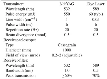
Table 1.Main specifications of USTC lidar system.
Transmitter: Nd:YAG Dye Laser
Wavelength (nm) 532 589
Pulse energy (mJ) 550 60 (typ.)
Line width (cm−1) 1 0.05
Pulse width (ns) 6 6
Repetition rate (Hz) 20 20
Beam divergence (mrad) 0.5 0.5 Receiver-telescope:
Type Cassegrain
Diameter (mm) 1000
Field of view (mrad) 0.2–2 (adjustable) Receiver-filter:
Wavelength (nm) 532 589
Bandwidth (nm) 1.0 0.5
Peak transmission ≥60% 70%
studies on SSLs by lidars were conducted after the observa-tion by Von Zahn and Hansen (1988) (e.g. Kwon et al., 1988; Batista et al., 1989; Senft et al., 1989; Kane et al., 1991; Gardner et al., 1993; Clemesha, 1995; Clemesha et al., 1998; Qian et al., 1998; Gong et al., 2002; Clemesha et al., 2004; Williams et al., 2006, 2007; Fan et al., 2007; Nesse et al., 2008; Vishnu Prasanth et al., 2007; Yi et al., 2007; Heinrich et al., 2008).
Sporadic sodium layers have been studied for more than 20 years. Before the 1990s, SSLs were known to be common at low and high latitudes, but rare at mid-latitudes. Kwon et al. (1988) saw 16 SSLs in 30 h of observations at Mauna Kea (19◦50′N), and Hansen and von Zahn (1990) saw 75 SSLs in 378 h of measurement at Andoya (69◦N). At 23◦S Batista et al. (1989) saw 65 SSLs in 3500 h of observations, and at Illinois (40◦N) Senft et al. (1989) saw only 2 SSLs in 350 h. No SSLs were reported from mid-latitude measurements by Gibson and Sandford (1971) and Megie and Blamont (1977). But subsequent observations showed that the mid-latitude deficit was not thought to be real in recent years. For ex-ample, measurements in the Eastern Hemisphere, i.e., Tokyo (35◦N) from November 1991 to October 1993 and Wuhan (31◦N) from February 1996 to August 2001, gave a mean oc-currence interval of about 10 h per SSL event (Nagasawa and Abo, 1995; Yi et al., 2002; Gong et al., 2002), and measure-ments in the Western Hemisphere, i.e., Colorado (40.6◦N) from April to June 2002 and June to August 2003, indicated that 65% of days and 19% of hours had SSLs (Williams et al., 2007). These observations showed much higher occurrence rates than those observed at mid-latitude before the 1990s. Williams et al. (2007) suggested that this possibly indicates a large interannual or decadal variability in the sporadic layer occurrence rate.
Recently, a Rayleigh-Sodium fluorescence lidar has been operated routinely in the campus of the Universtiy of Science and Technology of China (USTC), Hefei, China (31.8◦N,
117.3◦E)). From December 2005 to November 2008, 64 clear-cut SSLs were observed during 900 h of lidar measure-ments. A comprehensive statistical analysis of SSL events using nearly three years of sodium density observations by USTC lidar was done, and correlations to the sporadic-E lay-ers, together with their horizontal ranges estimated from the co-observational data obtained by two separated lidars are discussed.
2 Instrument description and data analysis
A Rayleigh-Sodium fluorescence lidar system was assem-bled, tested and deployed to the University of Science and Technology of China (USTC) at Hefei, China (31.8◦N, 117.3◦E) in December 2005, which is used for detecting atmospheric density and temperature and sodium density (Chen et al., 2007).
In sodium resonance fluorescence operating model, the transmitter is a tunable dye laser with 60 mJ pulse energy and 20 Hz repetition rate pumped by a Nd:YAG laser at second harmonic wavelength 532 nm. The dye laser is firstly tuned to the D2 resonant absorption line of sodium at 589 nm using a Na vapor cell, then the final fine tuning is accomplished by maximizing the signal backscattered from the sodium layer. The dye laser beam is always pointed at zenith, and the diver-gence of the beam is about 0.5 mrad. The backscattered pho-tons are collected by a 1 m diameter Cassegrain telescope. Passing through the appropriate narrow-band interference fil-ter, the backscattered photons are focused onto a photomul-tiplier tube (PMT), and then processed by a PC-based pho-ton counting multi-channel scalar (MCS) in successive time bins. The time bin length taken here is 100µs correspond-ing to a range bin length of 150 m. The photon counts from 5000 laser shots are accumulated to attain a lidar photocount profile, the corresponding time resolution for the photocount profile series is 250 s. The main characteristics of the USTC lidar are presented in Table 1.
Since the USTC lidar was built, we have carried on regu-lar observation of the sodium layer at Hefei. From December 2005 to November 2008, we accumulated a total observation time of 900 h from 118 nights. Among these, the SSL events were selected according to the following criteria: (1) The maximum density of SSL peak must be at least two times higher than that of the background sodium layer at the same altitude, and must be more than 1000 cm−3 if the altitude
(a) (b)
(c) (d)
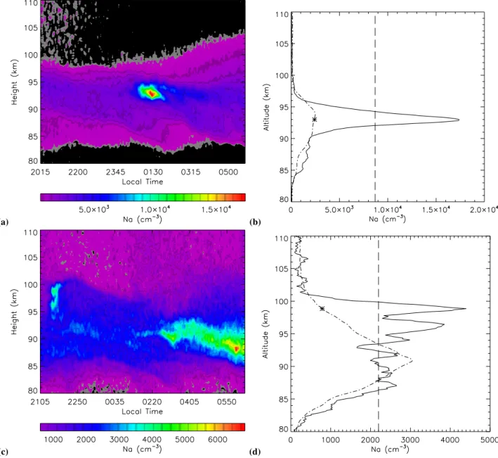
Fig. 1. Examples of the contour plots and the corresponding profiles at their maximum values of SSL events. (a–b)represent the SSL event on 20 March 2007, and(c–d)represent the SSL event on 27 January 2007. The dot-dashed lines in (b) and (d) indicate the averaged background sodium densities; the stars mark the background sodium densities corresponding to the sporadic sodium peak densities. The dashed lines show the half maximum values of the peak densities.
et al., 2004)). (3) It lasted for at least four successive lidar profiles (more than sixteen minutes). Following these condi-tions, 64 SSL events could be identified. More specifically, in the 900 h of measurements from about 118 nights, 64 SSL events were clearly identified in 57 nights.
3 Observations
Figure 1 shows examples of the contour plot and the single profile plot at the moment when a sporadic sodium layer reached its maximum density on 20 March 2007. It can
be observed from Fig. 1a that a local dense sodium layer appeared during 00:12–01:53 LT on 21 March 2007. The duration of the event lasted for about 100 min. From the profile at its maximum (Fig. 1b), one can measure its gen-eral characteristics, for example, the peak sodium density was 17 380 cm−3, the relevant altitude was 93.0 km, the full
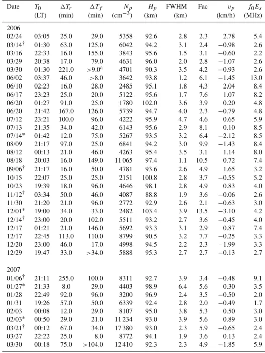
Table 2.List of the SSL events during 2006–2008.
Date T0 1Tr 1Tf Np Hp FWHM Fac vp f0Es
(LT) (min) (min) (cm−3) (km) (km) (km/h) (MHz) 2006
02/24 03:05 25.0 29.0 5358 92.6 2.8 2.3 2.78 5.4
03/14† 01:30 63.0 125.0 6042 94.2 3.1 2.4 −0.98 2.6 03/16 22:33 16.0 155.0 3843 95.6 1.5 3.1 −0.60 2.2
03/29 20:38 17.0 79.0 4631 96.0 2.0 2.8 −1.07 2.6
03/30 01:30 221.0 >9.0a 4701 90.3 3.5 4.2 −0.93 2.6 06/02 03:37 46.0 >8.0 3642 93.8 1.2 6.1 −1.45 13.0
06/10 02:23 16.0 28.0 2485 95.1 1.8 4.3 2.04 8.4
06/17 23:23 25.0 20.0 5122 95.6 1.7 7.6 1.07 8.2
06/20 01:27 91.0 25.0 1780 102.0 3.6 3.9 0.20 4.8
06/20 21:42 167.0 126.0 5739 94.7 4.0 2.3 −0.79 4.8
07/12 23:21 100.0 96.0 4222 95.9 4.7 4.6 0.65 5.9
07/13 21:35 34.0 42.0 6143 95.6 2.9 8.1 0.10 8.5
07/14∗ 01:42 12.0 75.0 5267 93.5 3.2 6.4 −2.12 8.5
08/09 21:17 97.0 25.0 6841 94.2 3.0 9.9 −1.43 8.4
08/12 00:13 21.0 46.0 4263 95.4 3.5 3.1 1.14 8.0
08/18 20:03 16.0 149.0 11 065 97.4 1.1 10.5 0.72 7.4
09/06† 21:17 16.0 50.0 4781 93.6 2.6 4.9 1.65 3.2
10/15 22:07 25.0 25.0 2151 100.8 2.8 3.7 −0.55 5.2
10/23 19:39 18.0 96.0 4646 98.1 2.8 4.9 0.83 4.0
11/12† 03:34 50.0 46.0 4087 88.8 1.9 3.6 −0.06 2.6
11/30 21:20 21.0 96.0 2772 92.9 2.6 2.1 −0.63 3.0
12/01∗ 19:00 34.0 33.0 2482 103.4 3.9 13.5 −3.10 4.2 12/14† 23:00 20.0 102.0 5511 93.2 2.7 3.6 −0.45 4.0
12/17 01:21 21.0 146.0 5692 93.3 3.1 2.9 0.87 7.4
12/17 22:45 113.0 110.0 8799 90.5 3.2 7.7 −0.25 3.3
12/20 23:00 46.0 17.0 4998 94.5 2.2 2.3 −1.99 3.3
12/29 19:47 33.0 >34.0 5888 95.3 2.7 2.7 −0.13 2.7
2007
01/06† 21:11 255.0 100.0 8311 92.7 3.9 3.4 −0.48 9.1
01/27∗ 21:33 8.0 29.0 4403 98.9 6.4 5.6 0.30 3.5
01/28 22:49 92.0 96.0 3200 96.9 2.4 3.5 −0.50 2.0
01/31 19:26 57.0 50.0 6339 92.4 2.8 2.0 −0.49 1.7
02/03 00:08 12.0 29.0 8107 95.0 3.8 5.3 0.50 3.0
02/03∗ 00:50 29.0 21.0 11 234 93.0 3.9 5.6 0.89 3.0 03/21† 00:12 67.0 34.0 17 380 93.0 2.3 5.9 −0.65 2.4
03/27 22:22 25.0 8.0 8772 94.1 1.9 3.6 0.13 2.4
03/30 00:18 75.0 >104.0 12 410 92.3 2.3 4.9 −1.85 5.9
The typical parameters of all 64 SSL events of USTC lidar observation, i.e., the beginning time of a SSL (T0), the
ris-ing time (1Tr, defined as the time elapsed between the first appearance of a SSL and its reaching maximum amplitude), the falling time (1Tf, defined as the time elapsed between the maximum amplitude to the last profile where the peak is still distinguishable), the maximum peak density of a SSL (Np), the corresponding altitude of the maximum peak den-sity (Hp), the width (FWHM), and the strength factor (Fac), are listed in the second to eighth columns of Table 2.
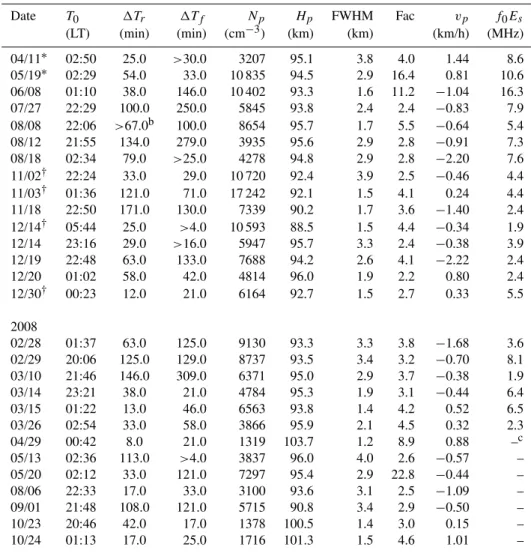
Table 2.Continued.
Date T0 1Tr 1Tf Np Hp FWHM Fac vp f0Es
(LT) (min) (min) (cm−3) (km) (km) (km/h) (MHz) 04/11∗ 02:50 25.0 >30.0 3207 95.1 3.8 4.0 1.44 8.6 05/19∗ 02:29 54.0 33.0 10 835 94.5 2.9 16.4 0.81 10.6 06/08 01:10 38.0 146.0 10 402 93.3 1.6 11.2 −1.04 16.3 07/27 22:29 100.0 250.0 5845 93.8 2.4 2.4 −0.83 7.9 08/08 22:06 >67.0b 100.0 8654 95.7 1.7 5.5 −0.64 5.4 08/12 21:55 134.0 279.0 3935 95.6 2.9 2.8 −0.91 7.3 08/18 02:34 79.0 >25.0 4278 94.8 2.9 2.8 −2.20 7.6 11/02† 22:24 33.0 29.0 10 720 92.4 3.9 2.5 −0.46 4.4 11/03† 01:36 121.0 71.0 17 242 92.1 1.5 4.1 0.24 4.4 11/18 22:50 171.0 130.0 7339 90.2 1.7 3.6 −1.40 2.4 12/14† 05:44 25.0 >4.0 10 593 88.5 1.5 4.4 −0.34 1.9 12/14 23:16 29.0 >16.0 5947 95.7 3.3 2.4 −0.38 3.9 12/19 22:48 63.0 133.0 7688 94.2 2.6 4.1 −2.22 2.4
12/20 01:02 58.0 42.0 4814 96.0 1.9 2.2 0.80 2.4
12/30† 00:23 12.0 21.0 6164 92.7 1.5 2.7 0.33 5.5
2008
02/28 01:37 63.0 125.0 9130 93.3 3.3 3.8 −1.68 3.6 02/29 20:06 125.0 129.0 8737 93.5 3.4 3.2 −0.70 8.1 03/10 21:46 146.0 309.0 6371 95.0 2.9 3.7 −0.38 1.9
03/14 23:21 38.0 21.0 4784 95.3 1.9 3.1 −0.44 6.4
03/15 01:22 13.0 46.0 6563 93.8 1.4 4.2 0.52 6.5
03/26 02:54 33.0 58.0 3866 95.9 2.1 4.5 0.32 2.3
04/29 00:42 8.0 21.0 1319 103.7 1.2 8.9 0.88 –c
05/13 02:36 113.0 >4.0 3837 96.0 4.0 2.6 −0.57 –
05/20 02:12 33.0 121.0 7297 95.4 2.9 22.8 −0.44 –
08/06 22:33 17.0 33.0 3100 93.6 3.1 2.5 −1.09 –
09/01 21:48 108.0 121.0 5715 90.8 3.4 2.9 −0.50 –
10/23 20:46 42.0 17.0 1378 100.5 1.4 3.0 0.15 –
10/24 01:13 17.0 25.0 1716 101.3 1.5 4.6 1.01 –
aLidar did not observe the end of SSL event bLidar did not observe the beginning of SSL event cNo corresponding data set
∗C-structure SSL event
†Wuhan Lidar had the corresponding observational data
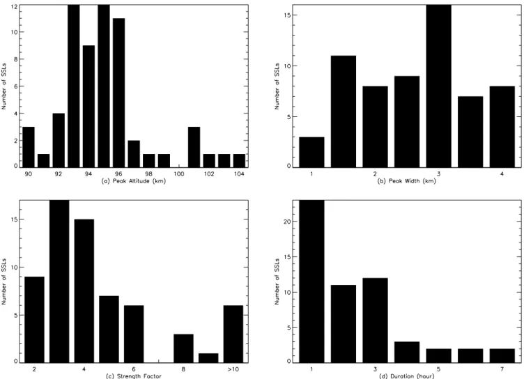
Figure 2b shows the distribution of the width of the 64 SSL events, which was around 1.0–4.0 km for most of the normal SSL events and had an average value of 2.6 km. One excep-tion was the case on 27 January 2007 as shown in Fig. 1c– d. One can find in Fig. 1c, that a structure like a reversed letter “C” appeared during 21:33 LT–22:10 LT between 95– 100 km, the width of this event was about 6.4 km (shown in Fig. 1d), the maximum width among all the SSL events. The so-called C-structure SSL event was first observed by Kane et al. (2001), and named by Clemesha et al. (2004). Actu-ally, we observed six C-structure SSL events (indicated by stars in Table 2): one was a reversed C-structure SSL, the other five were normal C-structure one. Because C-structure SSLs often showed complex height/time structures,
Fig. 2.Statistical plots of peak altitudes, width (FWHM), strength factors and durations for SSL events.
The strength factors of most SSL events were distributed within the range 2–6 as shown in Fig. 2c, with a relatively high value>10 for six events. In particular, the SSL event on 20 May 2008 had a strength factor of 22.8, due to the relatively lower sodium density above 95 km during non-sporadic period (average value∼400 cm−3).
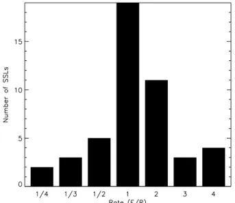
Figure 2d gives the distribution of the durations of the SSL events. This statistical plot excluded those events for which we did not observe the beginning times or ending times. One can find that most of them lasted for about 1–3 h. These re-sults agree with those reported by other sodium lidar groups (Batista et al., 1989; Yi et al., 2002; Gong et al., 2002; Vishnu Prasanth et al., 2007). Figure 3 shows the histogram distri-bution of the ratio of the falling times versus rising times for the SSL events analyzed in Fig. 2d, and it indicates that the falling times were a little longer than the rising times. The rising times ranged from 8 min to over 4 h with an average of 56 min, and the falling times ranged from 8 min to over 5 h with an average of 79 min. These values were in line with
those observed at 23◦S (i.e., Batista et al., 1989, showed the average rising times and falling times of SSLs were 50 min and 174 min, respectively), but were generally longer than those seen at low latitude (i.e., Kwon et al., 1988, observed fifty percent of the SSLs had apparent rising times of less than 10 min, and about 2/3 of the falling times were greater than 10 min, with 1/3 greater than 20 min) and high latitude (i.e., von Zahn et al., 1987, illustrated that the SSLs increased by large factors within a few minutes). Most of observa-tions proved that the rising times were shorter than falling times, but Vishnu Prasanth et al. (2007) have seen longer ris-ing times of about 48 min on an average and shorter fallris-ing times with an average of 30 min.
Fig. 3.Statistical plot of the Rate of Falling time (F) to Rising time (R).
more frequent occurrence near midnight. Previous studies showed that the occurrence was concentrated near midnight for high-latitude SSLs (Hansen and von Zahn, 1990; Hein-rich et al., 2008), but had a relatively wide distribution ver-sus local time for low- and mid-latitude SSLs (Batista et al., 1989; Clemesha, 1995; Vishnu Prasanth et al., 2007; Gong et al., 2002). This was also true from our observations. It is worth mentioning that observations at night with limited op-eration hours can not reveal the whole local-time dependence of SSLs, thus the specific timing of dataset and analyzing all the sodium datasets in the same fashion must be accounted for in order to understand the variations of SSLs better.
Another statistical parameter is the velocity of the trajecto-ries of the sporadic sodium peak as shown in the 9th column of Table 2 and Fig. 5, which was obtained by linear fitting of the height-time relation for SSL peaks on a given night. The positive and negative velocities represent the upward and downward motions of SSL peaks, respectively. The veloci-ties were considered as zero if they are between±0.5 km/h. In this situation, we deemed the sporadic layer to be “sta-ble”. For all these 64 SSL events, 22 events were “stable” versus time, 25 events showed downward motions with av-erage velocities−1.25 km/h, and 17 events showed upward motions with average velocities near 1.08 km/h. Batista et al. (1989) found most SSLs showed downward motion with a rate of 1 km/h at 23◦S. The observations of Kwon et al. (1988) at Mauna Kea showed a typical rate of descent about twice of that observed by Batista et al., and Vishnu Prasanth et al. (2007) also reported a downward motion with a veloc-ity 2 km/h. At the same time, Gong et al. (2002) supported the results observed by Batista et al. (1989), and according to their observations at Wuhan, downward motions occurred
Fig. 4.Statistical plot of the SSL occurrence time.
Fig. 5. Statistical plot of the average velocity of the SSL peaks trajectories. Positive and negative values represent the upward and downward motions of SSL peaks, respectively.
more often than upward ones (about 4 times more). These re-sults were a little different from our lidar observations, which shows that SSLs are perturbed by local dynamics processes of the atmosphere during their development.
4 Discussion and conclusions
Fig. 6. Co-observation of USTC lidar (upper panel) and WIPM lidar (bottom panel) for an SSL event on 2 November 2007 at Hefei and Wuhan.
Table 3. Seasonal variations of probability of occurrence of SSL andES.
Month Total Obs. SSL No. SSL Occurrence f0Es>5 MHz
(Hour) (Hour) (Hour per SSL) (%)
Jan 69.9 4 17.5 3.39 Feb 46.9 5 9.4 3.32 Mar 117.8 11 10.7 1.65 Apr 44.4 2 22.2 5.92 May 43.8 3 14.6 31.84 Jun 38.6 6 6.4 36.20 Jul 21.0 4 5.2 28.86 Aug 76.3 7 10.9 22.75 Sep 24.7 2 12.3 5.42 Oct 82.1 4 20.5 4.28 Nov 166.0 5 33.2 0.91 Dec 168.0 11 15.3 2.52
Total 899.4 64 14.1 12.26
Seasonal variations of occurrence of SSL events are listed in 4th column in Table 3, which were obtained from dividing the total observational time of a given month (2nd column in Table 3) by the numbers of the SSL events (3rd column in Table 3). One can infer that SSL had a high frequency about 1 event per 6 h during summer months, especially in June and July, and a lowest frequency (1 event every 33.2 h) during November.
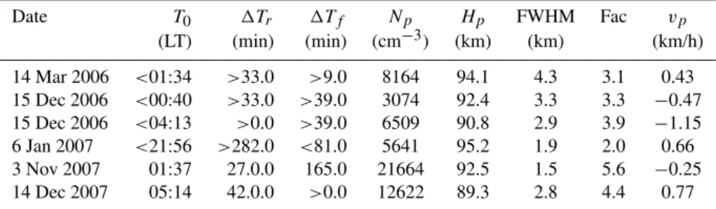
Table 4.Parameters of five co-observational SSL events observed at Wuhan by WIPM lidar.
Date T0 1Tr 1Tf Np Hp FWHM Fac vp
(LT) (min) (min) (cm−3) (km) (km) (km/h) 14 Mar 2006 <01:34 >33.0 >9.0 8164 94.1 4.3 3.1 0.43 15 Dec 2006 <00:40 >33.0 >39.0 3074 92.4 3.3 3.3 −0.47 15 Dec 2006 <04:13 >0.0 >39.0 6509 90.8 2.9 3.9 −1.15 6 Jan 2007 <21:56 >282.0 <81.0 5641 95.2 1.9 2.0 0.66 3 Nov 2007 01:37 27.0.0 165.0 21664 92.5 1.5 5.6 −0.25 14 Dec 2007 05:14 42.0.0 >0.0 12622 89.3 2.8 4.4 0.77
Nagasawa and Abo, 1995). Recognition of the relationship between SSL and Es events may prove to be an important ad-ditional clue regarding the origins of both layering processes. In order to study the correlation between SSL and Es dur-ing our observational period, we employed the correspond-ing f0Es data from an ionosonde at Yamagawa (31.2◦N, 130.5◦E) from January 2006 to March 2008. The maximum values off0Es at the corresponding night of SSL events are listed in the last column of Table 2. Due to the long hori-zontal distance between Hefei and Yamagawa (∼1000 km), the statistical analysis will be more illustrative. We counted the occurrence off0Es>5 MHz from sunset to sunrise of ev-ery month at Yamagawa; the results are listed in the last col-umn of Table 3. One can see the considerable correlation between seasonal variations of occurrence of SSL and those of Es during nighttime. The linear Pearson correlation coeffi-cient between the inverse of SSL occurrences in Table 3 (i.e., the numbers of SSL events per hour) and the occurrences of f0Es>5 MHz is 0.66.
Up to now, there have been few published results con-cerning the horizontal ranges of SSLs. One exception was a study of 19 SSLs at 23◦S using a steerable lidar (Batista et al., 1991), where the horizontal dimensions of the Na clouds were found to be between 100 and 2000 km. An airborne lidar (ALOHA90) has also been used to show that an SSL in the Pacific equatorial region extended for more than 1800 km (Kane et al., 1991). Another airborne obser-vation (ALOHA/ANLC-93) showed that the horizontal ex-tents varied from approximately 25 to almost 1600 km with a mean of 440 km (Qian et al., 1998). Recently, satellite-borne measurements illustrated that most SSLs were much more prevalent in the Southern Hemisphere, with a horizon-tal extent of less than 300 km (Fan et al., 2007). The Wuhan Institute of Physics and Mathematics (WIPM) built the first sodium lidar system in China in 1996 (Gong et al., 2002), which is located at Wuhan (31◦N, 114◦E) about 500 km away from Hefei. In suitable weather conditions, the WIPM lidar and the USTC lidar can provide latitude horizontal co-observation of sodium layer.
Figure 6 shows an SSL event observed on 2 November 2007 by the USTC lidar and the WIPM lidar together. The corresponding observational time interval for the USTC
li-dar and the WIPM lili-dar were 19:25–05:55 LT and 22:25– 05:55 LT. There were two SSL events detected by the USTC lidar, one developed from 22:24–23:26 LT and the other from 01:36 LT–04:48 LT. However, the first SSL event was not de-tected by the WIPM lidar, and only the last one was observed by the WIPM lidar from 01:37–04:49 LT. The duration, ap-pearance altitude, and strength of this SSL event were very consistent with those of observed by the USTC lidar.
We checked the WIPM lidar observational data, and for the 57 nights listed in Table 2, there were a total of nine nights (indicated by “†” in Table 2) on which the WIPM lidar had co-observational data. But for the days, i.e., 6 September 2006, 20 March 2007, and 29 December 2007, the observations of the WIPM lidar did not cover the periods of SSL developments (the corresponding observational peri-ods of the WIPM lidar were 23:40–00:01 LT on 6 September 2006, 02:14–03:17 LT on 20 March 2007, 18:36–19:18 LT and 04:24–05:18 LT on 29 December 2007). Also, for 12 November 2006, the observations of the WIPM lidar (from 00:20–03:50 LT) just covered the beginning time of SSL ob-served by the USTC lidar and no evident SSL event had been observed. Thus, these four days were excluded and only five days were used here.
The typical parameters of SSL events observed by the WIPM lidar, that is, the beginning time (T0), the rising time
(1Tr), the falling time (1Tf), the maximum peak density (Np), the altitude of the maximum peak density (Hp), width (FWHM), and the strength factor (Fac), are listed in Table 4. Since the observational period only covered some time inter-vals instead of the whole night, the WIPM lidar did not detect the whole process of the SSL developments for some events listed in Table 4 (“<” indicated that the beginning time was not observed, and “>” indicates that the corresponding peri-ods were longer than those shown in Table 4).
densities and the peak velocities for the same event were dif-ferent from each other; this may be the result of the local mid-dle atmospheric dynamics (Note that there were greater dif-ferences for peak altitude and width on 6 January 2007, the contour plots for the two locations showed that SSL had been broadened at Hefei during its maximum period. We con-sidered that this can also be explained by the local dynam-ical process). Still, there were two events that were not ob-served simultaneously, i.e., event from 22:24–23:26 LT on 2 November 2007 (as shown in Fig. 6), and event from 04:13– 04:52 LT on 14 December 2006 (as shown in Table 4). Ow-ing to the lack of a third observational lidar, it cannot be de-termined from our two-point observation, whether these two events were very local phenomena.
To summarize, we did a comprehensive statistical analysis of SSL events using nearly three years of sodium density ob-servations by the USTC lidar. The results are in agreement with those reported by previous studies at mid-latitude. With the help of ionosonde data, a considerable correlation with Pearson correlation coefficient 0.66 between seasonal varia-tions of occurrence of SSL and those of Es during nighttime can be obtained, which was in line with the research made by Nagasawa and Abo (1995). From a comparison between the observations of the USTC lidar and the WIPM lidar, the least horizontal range for some events was estimated to be over 500 km. We consider that more co-observations will greatly help us understand the horizontal ranges of SSL, and more comprehensive results can be obtained with the support of China Median Project (a national scientific project funded by the Ministry of Science and Technology of China. It is a comprehensive ground-based system to monitor space en-vironment variations occurring in the middle-to-upper atmo-sphere, the ionoatmo-sphere, etc., based on many instruments and a network of facilities, along a 120◦E meridian chain, from Mohe, the northernmost station in China, and extending to the China Zhongshan station in the Antarctic; and a 30◦N latitudinal chain, from the easternmost point at Shanghai to the western Lhasa station) which is under construction.
Acknowledgements. We thank the Yamagawa Observatory for their
f0Es data, and the Wuhan Institute of Physics and Mathemat-ics (CAS) for their sodium layer observation data used in this paper. We also wish to thank referees for suggesting a num-ber of substantial improvements in the manuscript. This work is supported by the grant of the Creative Program (kzcx2-yw-123) and the grant of the President Scholarship of Chinese Academy of Sciences, the National Natural Science Foundation of China (40804035, 40674087,40890165), Program for New Century Ex-cellent Talents in University (NCET-08-0523), the China Meteoro-logical Administration Grant (GYHY200706013), and the Innova-tion Program of the Chinese Academy of Sciences (IAP07307).
Topical Editor C. Jacobi thanks B. P. Williams and another anonymous referee for their help in evaluating this paper.
References
Batista, P., Clemesha, B., Batista, I., and Simonich, D.: Characteris-tics of the sporadic sodium layers observed at 23◦S, J. Geophys. Res., 94, 15349–15358, 1989.
Batista, P. P., Clemesha, B. R., and Simonich, D. M.: Horizon-tal structures in sporadic sodium layers at 23◦S, Geophys. Res. Lett., 18, 1027–1030, 1991.
Bills, R. E. and Gardner, C. S.: Lidar observations of the mesopause region temperature structure at Urbana, J. Geophys. Res., 98, 1011–1021, 1993.
Bills, R. E., Gardner, C. S., and Franke, S. J.: Na Doppler/temperature lidar: Initial mesopause region observa-tions and comparison with the Urbana medium frequency radar, J. Geophys. Res., 96, 22701–22707, 1991.
Bowman, M. R., Gibson, A. J., and Sandford, M. C. W.: Observa-tion of mesospheric Na atoms by tuner laser radar, Nature, 221, 456–458, 1969.
Chen, T., Xue, X., and Dou, X.: Lidar studies of nighttime sodium layer over Hefei, China, J. Univ. of Sci. & Tech. of China, 37, 873–878, 2007.
Clemesha, B.: Sporadic neutral metal layers in the mesosphere and lower thermosphere., J. Atmos. Solar-Terres. Phys., 57, 725–736, 1995.
Clemesha, B., Kirchhoff, V., Simonich, D., and Takahashi, H.: Ev-idence of an extraterrestrial source for the mesospheric sodium layer., Geophys. Res. Lett., 5, 873–876, 1978.
Clemesha, B., Kirchhoff, V., Simonich, D., Takahashi, H., and Batista, P.: Spaced lidar and nightglow observations of an atmo-spheric sodium enhancement., J. Geophys. Res., 85, 3480–3484, 1980.
Clemesha, B., Simonich, D., Batistu, P., and Batista, I.: Lidar ob-servation of atmospheric sodium at an equatorial location., J. At-mos. Solar-Terr. Phys., 60, 1773–1778, 1998.
Clemesha, B., Batista, P. P., Simonich, D. M., and Batista, I. S.: Sporadic structures in the atmospheric sodium layer, J. Geophys. Res., 109, D11306, doi:10.1029/2003JD004496, 2004.
Collins, S. C., Plane, J. M. C., Kelley, M. C., Wright, T. G., Soldan, P., Kane, T. J., Gerrard, A. J., Grime, B. W., Rollason, R. J., Friedman, J. S., Gonzalez, S. A., Zhou, Q. H., Sulzer, M. P., and Tepley, C. A.: A study of the role of ion-molecule chemistry in the formation of sporadic sodium layers, J. Atmos. Sol.-Terr. Phys., 64, 845–860, 2002.
Cox, R. and Plane, J.: An ion-molecule mechanism for the forma-tion of neutral sporadic Na layers., J. Geophys. Res., 103, 6349– 6359, 1998.
Cox, R. M., Self, D. E., and Plane, J. M. C.: A study of the reaction between NaHCO3 and H: Apparent closure on the chemistry of mesospheric Na, J. Geophys. Res., 106, 1733–1739, 2001. Fan, Z. Y., Plane, J. M. C., and Gumbel, J.: On the global
distribu-tion of sporadic sodium layers, Geophys. Res. Lett., 34, L15808, doi:10.1029/2007GL030542, 2007.
Gardner, C., Kane, T., Senft, D., Qian, J., and Papen, G.: Simultane-ous observations of sporadic E, Na, Fe, and Ca+ layers at Urbana, Illinois: three case studies., J. Geophys. Res., 98, 16865–16874, 1993.
Gardner, C. S. and Shelton, J. D.: Density response of neutral at-mospheric layers to gravity wave perturbations, J. Geophys. Res., 90, 1745–1754, 1985.
sodium layer over Urbana , Illinois : 2. Gravity waves, J. Geo-phys. Res., 92, 4673–4694, 1987.
Gardner, C. S., Plane, J. M. C., Pan, W., Vondra, T., Murray, B. J., and Chu, X.: Seasonal variations of the Na and Fe layers at the South Pole and their implications for the chemistry and gen-eral circulation of the polar mesosphere, J. Geophys. Res., 110, D10302, doi:10.1029/2004JD005670., 2005.
Gibson, A. J. and Sandford, C.: The seasonal variation of the night-time sodium layer, J. Atmos. Terr. Phys., 33, 1675–1684, 1971. Gong, S., Yang, G., Wang, J., Liu, B., Cheng, X. W., Xu, J. Y.,
and Wan, W.: Occurrence and characteristics of sporadic sodium layer observed by lidar at a mid-latitude location, J. Atmos. Solar-Terr. Phys., 64, 1957–1966, 2002.
Hansen, G. and von Zahn, U.: Sudden sodium layers in polar lati-tudes, J. Atmos. Terr. Phys., 52, 585–608, 1990.
Heinrich, D., Nesse, H., Blum, U., Acott, P., Williams, B., and Hoppe, U.-P.: Summer sudden Na number density enhancements measured with the ALOMAR Weber Na Lidar, Ann. Geophys., 26, 1057–1069, 2008,
http://www.ann-geophys.net/26/1057/2008/.
Hickey, M. P. and Plane, J. M. C.: A chemical-dynamical model of wavedriven sodium fluctuations, Geophys. Res. Lett., 22, 2861– 2864, 1995.
Kane, T., Grime, B., Franke, S., Kudeki, E., Urbina, J., Kelley, M., and Collins, S.: Joint observations of sodium enhancements and field aligned ionospheric irregularities., Geophys. Res. Lett., 28, 1375–1378, 2001.
Kane, T. J., Hostetler, C. A., and Gardner, C. S.: Horizontal and vertical structure of the major sporadic sodium layer events ob-served during ALOHA-90, Geophys. Res. Lett., 18, 1365–1368, 1991.
Kwon, K., Senft, D., and Gardner, C.: Lidar observations of spo-radic sodium layers at Mauna Kea Observatory, Hawaii, J. Geo-phys. Res., 93, 14199–14208, 1988.
Kwon, K. H., Gardner, C. S., and Senft, D. C.: Daytime lidar mea-surements of tidal winds in the mesospheric sodium layer at Ur-bana, Illinois, J. Geophys. Res., 92, 8781–8786, 1987.
Mathews, I., Zhou, Q., Philbrich, C., Morton, Y., and Gardner, C.: Observations of ion and sodium layer coupled processes during AIDA., J. Atmos. Terr. Phys., 55, 487–498, 1993.
Megie, M. and Blamont, J. E.: Laser sounding of atmospheric sodium interpretation in terms of global atmospheric parameters, Planet. Space Sci., 25, 1093–1109, 1977.
Nagasawa, C. and Abo, M.: Lidar observations of a lot of sporadic sodium layers in mid-latitude., Geophys. Res. Lett., 22, 263–266, 1995.
Nesse, H., Heinrich, D., Williams, B., Hoppe, U.-P., Stadsnes, J., Rietveld, M., Singer, W., Blum, U., Sandanger, M. I., and Trond-sen, E.: A case study of a sporadic sodium layer observed by the ALOMAR Weber Na lidar, Ann. Geophys., 26, 1071–1081, 2008, http://www.ann-geophys.net/26/1071/2008/.
Papen, G. C., Pfenninger, W. M., and Simonich, D. M.: Sensitiv-ity analysis of Na narrowband wind-temperature lidar systems, Appl. Optics, 34, 480–498, 1995.
Plane, J. M., Gardner, C. S., Yu, J., She, C. Y., Garcia, R. R., and Pumphrey, H. C.: Mesospheric Na layer at 40N: Modeling and observations., J. Geophys. Res., 104, 3773–3788, 1999. Vishnu Prasanth, P., Sridharan, S., Bhavani Kumar, Y., and
Narayana Rao, D.: Lidar observations of sporadic Na layers over
Gadanki (13.5◦N, 79.2◦E), Ann. Geophys., 25, 1759–1766, 2007, http://www.ann-geophys.net/25/1759/2007/.
Qian, J., Gu, Y., and Gardner, C.: Characteristics of the spo-radic Na layer observed during the Airborne Lidar and Ob-servations of Hawaiian Airglow/Airborne Noctilucent cloud (ALOHA/ANLC-93) campaigns., J. Geophys. Res., 103, 6333– 6347, 1998.
Senft, D., Collins, R., and Gardner, C.: Mid-latitude lidar observa-tions of large sporadic sodium layers., Geophys. Res. Lett., 16, 715–718, 1989.
She, C. Y., Yu, J. R., Latifi, H., and Bills, R. E.: High-spectral-resolution fluorescence light detection and ranging for meso-spheric sodium temperature measurements, Appl. Optics, 31, 2095–2106, 1992.
She, C. Y., Chen, S. S., Hu, Z. L., Sherman, J., Vance, J. D., Va-soli, V., White, M. A., Yu, J. R., and Krueger, D. A.: Eight-year climatology of nocturnal temperature and sodium density in the mesopause region (80 to 105 km) over Fort Collins, CO (41 N, 105 W), Geophys. Res. Lett., 27, 3289–3292, 2000.
Simonich, D. M., Clemesha, B. R., and Kirchhoff, V. W. J. H.: The mesospheric sodium layer at 23 S: Nocturnal and seasonal varia-tions., J. Geophys. Res., 84, 1543–1550, 1979.
States, R. J. and Gardner, C. S.: Structure of the mesospheric Na layer at 40◦N latitude: Seasonal and diurnal variations, J. Geo-phys. Res., 104, 11783–11798, 1999.
Swider, W.: Mesospheric sodium: Implications using a steady-state model, Planet. Space Sci., 34, 603–608, 1986.
Von Zahn, U. and Hansen, T.: Sudden neutral sodium layers: a strong link to sporadic E layers., J. Atmos. Terr. Phys., 50, 93– 104, 1988.
von Zahn, U., von der Gathen, P., and Hansen, G.: Forced release of sodium from upper atmospheric dust particles, Geophys. Res. Lett., 14, 76–79, 1987.
Williams, B. P., Croskey, C. L., She, C. Y., Mitchell, J. D., and Gold-berg, R. A.: Sporadic sodium and E layers observed during the summer 2002 MaCWAVE/MIDAS rocket campaign, Ann. Geo-phys., 24, 1257–1266, 2006,
http://www.ann-geophys.net/24/1257/2006/.
Williams, B. P., Berkey, F. T., Sherman, J., and She, C. Y.: Coinci-dent extremely large sporadic sodium and sporadic E layers ob-served in the lower thermosphere over Colorado and Utah, Ann. Geophys., 25, 3–8, 2007,
http://www.ann-geophys.net/25/3/2007/.
Xu, J. and Smith, A. K.: Perturbations of the sodium layer: con-trolled by chemistry or dynamics?, Geophys. Res. Lett., 30(20), 2056, doi:10.1029/2003GL018040, 2003.
Yi, F., Zhang, S., Yu, C., He, Y., Yue, X., Huang, C., and Zhou, J.: Lidar observations of sporadic Na layers over Wuhan (30.5 N, 114.4 E), Geophys. Res. Lett., 29(9), 1345, doi:10.1029/2001GL014 353, 2002.
Yi, F., Zhang, S., Yu, C., He, Y., Yue, X., Huang, C., and Zhou, J.: Simultaneous observations of sporadic Fe and Na lay-ers by two closely colocated resonance fluorescence lidars at Wuhan (30.5 N, 114.4 E), China, J. Geophys. Res., 112, D04303, doi:10.1029/2006JD007413, 2007.