Orographic effects on convective precipitation and space-time rainfall variability: preliminary results

285

Orographic effects on convective precipitation and space-time

rainfall variability: preliminary results

Paolina Bongioannini Cerlini

1,2

_{, Kerry A. Emanuel}

1

_{and Ezio Todini}

3

1,2_{Dept. Earth Atmospheric and Planetary Sciences, MIT Cambridge, USA} 2

Dept. of Physics, University of Perugia, Italy

3_{Dept. of Earth and Geo-Environmental Sciences, University of Bologna, Italy}

E-mail for corresponding author:cerlini@fisica.unipg.it

Abstract

In the EFFS Project, an attempt has been made to develop a general framework to study the predictability of severe convective rainfall events in the presence of orography. Convective activity is embedded in orographic rainfall and can be thought as the result of several physical mechanisms. Quantifying its variability on selected area and time scales requires choosing the best physical representation of the rainfall variability on these scales. The main goal was (i) to formulate a meaningful set of experiments to compute the oscillation of variance due to convection inside model forecasts in the presence of orography and (ii) to give a statistical measure of it that might be of value in the operational use of atmospheric data. The study has been limited to atmospheric scales that span the atmosphere from 2 to 200 km and has been focused on extreme events with deep convection. Suitable measures of the changing of convection in the presence of orography have been related to the physical properties of the rainfall environment. Preliminary results for the statistical variability of the convective field are presented.

Keywords: convection, orographic rainfall, predictability of precipitation, radiative–convective equilibrium

Introduction

The variability of precipitation in space and time depends on various factors, including the ambient thermodynamic structure of the atmosphere and its interaction with large-scale atmospheric circulations. Reproduction of precipitation space–time variability requires an understanding of the atmospheric mechanisms that may account for such variation. Numerical models of precipitation have different representations of the mechanisms involved, depending on the way account is taken of atmospheric convection inside flow dynamics. High resolution models that simulate convection explicitly (Cloud Resolving Models, CRM) are commonly used to reproduce observed precipitation fields; they are believed to provide realistic rainfall fields and, therefore, to give reliable estimates of precipitation variability.

However, the spatial and temporal horizon of predictability connected to precipitation fields is still difficult to estimate in many cases (e.g. Kaufmann et al., 2003; Richard et al., 2003), especially when convective motions

are involved. When moist convection is simulated by convective and mesoscale resolving numerical models, clouds are initiated and maintained through two main mechanisms: the release of convective available potential energy (CAPE), which depends on boundary and initial conditions and a continuous forcing by specified large-scale conditions which destabilises the atmosphere to convection. In the first case, convection depends crucially on whether or not there is a capping inversion, or negative area on soundings, and its time-scale is compared to that over which convection equilibrates its environment. In the second case, convective clouds are simulated over a long enough time to allow the ensemble of clouds to be in statistical equilibrium with the forcing, and the generation of CAPE by large-scale processes is nearly balanced by consumption due to convective motions. In this latter case, the convection time-scale can be considered small compared to those over which the forcing is likely to vary.

286

simulations of mesoscale convection from a typical thermodynamic and kinematic environment, starting from complete observed fields, or from an infinitesimal perturbation which destabilises the atmosphere to convection. In the first two cases, where the simulated field is strongly dependent on the initial condition, an observed structure is imposed on the developing system. In the third case, any structure may be imposed on the developing perturbations; therefore, it is the dynamic mechanism of forcing that runs the system to an equilibrium state, which is not reminiscent of the initial thermo-dynamical state but eventually evolves to one of statistical equilibrium.

Within the EFFS Project (E_uropean F_lood F_orecasting S_{ystem, EFFS), the second case of initialisation has been}

chosen for the high space–time resolution of atmospheric simulations. The simulations are for case studies of floods arising from specific heavy rainfall events derived from an ensemble of initial conditions (IC) given by precipitation forecast by the ECMWF GCM model. These simulated case studies are strongly dependent on the dynamic and thermo-dynamic environment, particularly when precipitation, measured by raingauge stations in mountainous regions, is compared with high resolution, numerically-simulated precipitation fields for the same area and time period (see EU reports: http://effs.wldelft.nl).

Thus, a number of questions can be asked when a different initialisation of convective activity is used, starting from an initially simple atmospheric state. Firstly, is it possible to formulate a meaningful experiment that reproduces minimal large-scale forcing destabilising the atmosphere to convection that is independent of the initial condition (and even using dynamically different models)? Secondly, can the oscillation of variance due to convective activity in model forecasts be computed, once the atmosphere has reached a statistically stable state? Finally, what is the effect on the convective activity and precipitation when the statistical equilibrium state between convection and the simulated dynamic mechanism of forcing is perturbed by changing the lower boundary condition with a mountain?

This paper presents a statistical evaluation, firstly, of the radiative-convective equilibrium state reached by the atmosphere and, secondly, of the effect of orographic forcing on the variability of precipitation, if this latter effect has to be taken into account among the dynamic and thermo-dynamic factors controlling convection.

Experiments on statistical equilibrium

of a convective atmosphere

To account for the convective variance of the rainfall field independently of the models’ initial conditions, convection

has to be simulated starting from a dynamic condition where convective activity is stable, statistically, and the physical system is in equilibrium. The basic assumption in all these experiments is statistical equilibrium of the convective atmosphere (see Emanuel et al., 1994; Robe and Emanuel, 1996); it is generally correct in tropical atmospheres where deep convection tends to develop but it is not restrictive. Indeed, the theory about convection holds for mid-latitude continents in summer when convective clouds dominate the thermodynamic structure of the atmosphere (Emanuel, 1994). It also holds in the case of synoptic flows where convection is embedded in the orographic updraught due to the presence of mountains and flow over them (Buzzi et al., 1998). The present experiment on convective variability, from an initial dynamic state, addresses the dynamic and thermodynamic effects introduced subsequently in the simulations.

For this purpose, a convective-scale resolving model, non-hydrostatic, with explicit resolution of moisture variables, such as ARPS (A_dvanced R_egional P_rediction S_{ystem, Xue}

et al., 1993) has been adapted to the proposed research. The choice of parameters and boundary conditions (BCs) in the ARPS model follows Robe and Emanuel (1996); it is suitable for simulating convective cells and systems in a three-dimensional structure and for accounting for the variance of convective rainfall thereafter.

287 Figure 1 shows the energy fluxes for the convective flow

when surface fluxes and radiative cooling are in balance, i.e. when the sum of fluxes oscillates around zero within the interval in which the fluxes are measured. Because of the impossibility of modelling the entire globe with convective dynamic features resolved, as well as the need to deal with the interaction with ‘large-scale’ features of atmospheric circulation not represented in the model domain, the intrinsic space- and time-scales of the convective ensemble have to be established (Tompkins and Craig, 1998). To calculate statistics for this ensemble, the development or lifespan of not only a single cloud but also of many of them in a state of equilibrium has to be considered.

Then, there are two main reasons for the oscillation in the balance of fluxes. Firstly, this state is said to be of statistical energy equilibrium with moist convection and, as stated by Arakawa and Schubert (1974), is such that the time-scale

over which the turbulent kinetic energy (one of the model’s prognostic variables) of moist convection adjusts to changes in large-scale forcing is small compared to that over which the forcing evolves. Since, in the present experiments, fields such as surface fluxes are sampled on a time-scale equivalent to the life-time of convective clouds (0.5 hour), the equilibrium profile shows that the oscillation due to convective activity is well below the time-scale on which the large-scale forcing (radiative cooling) is applied (days). Secondly, this energy balance equilibrium is achieved by a numerical simulation where the dynamic factors that must equilibrate on these different time-scales are approximated numerically; in these simulations, strong radiative cooling speeds up the equilibrium and introduces a numerical approximation to the theoretical results.

One of the problems in defining an equilibrium state for convection from which to start the experiments was to define which physical situation can reproduce the oscillation of

288

the convective activity, without specifying it and, then, relying on the large-scale forcing imposed. The intrinsic space- and time-scales of the convective ensemble will depend upon the organisation of the convection, itself dependent on large-scale environmental factors such as vertical wind shear. Then, a very essential setting for convection without vertical shear or even mean wind has been used to quantify the oscillation, related intrinsically to the convective field, on a space- and time-scale large enough to encompass an ensemble of clouds and not constrained in an unrealistic way. The number of horizontal grid points needed to avoid constraining the behaviour of the convective ensemble can be computed (Tompkins and Craig, 1998) using the mass continuity equation, the energy balance condition and the dimensional scaling for the CAPE that determines the cumulus velocity activity. The result is that, for some estimated climatological values for the CAPE, the number of grid points to maintain continuous convection is about s–1 _{= 2400, corresponding to a dimension of about}

50 × 50 grid points in the horizontal. A grid of 66 × 66 horizontal grid points with a 2 km resolution and a vertical resolution of 0.5 km for 41 grid points was, therefore, chosen for the first part of this study; it also takes account of the strong radiative cooling rate of the atmosphere (5.4 Kday–1_).

However, the results of simulations performed on a larger domain in the second part of this study will also be presented. The vertical fixed cooling applied to the atmosphere constitutes a strong constraint for convection to develop. Indeed, the radiative cooling is how, in the numerical atmospheric model, it is possible to simulate the net cooling due to the interaction of clouds with the radiative field along with the adiabatic cooling due to large-scale ascent of air. This high cooling rate, imposed to reach the equilibrium state more quickly, requires a domain size similar to that selected to allow both organised convection and single cells to develop and to ensure that the ensemble of clouds is not forced in an unrealistic way.

CONVECTIVE VARIABILITY

The first part of the experiment was to evaluate the statistical oscillation of convective activity for an ensemble of clouds at statistical equilibrium. To quantify convective variability, this study focused on extreme precipitation events with deep convection; it was, therefore, limited to scales that span the atmospheric g and b Mesoscale (2–200 km, after Orlansky, 1975) where cumulus clouds are resolved in a numerical domain large enough to contain many convective events. However, in the first place, these simulations were limited to a smaller domain for the reasons explained earlier.

The experiment was run for long enough for the

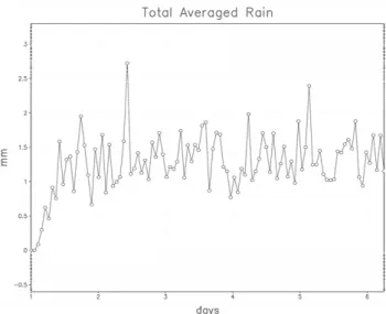
domain-averaged precipitation to come into statistical equilibrium. Atmospheric flow reached a stable configuration as displayed by the stable horizontally-averaged vertical profiles of potential temperature, relative humidity and entropy-related variables such as moist static energy (not shown). After a spin-up time, depending on the rate of radiative cooling applied, the system became a statistically equilibrated convective atmosphere where shallow and deep clouds form, grow and die continuously. Therefore, at equilibrium a moving average of rainfall intensity should be close to the surface evaporation rate, although individual fluctuations around the precipitation mean can be large, corresponding to the time-scale of the ensemble of cumulus clouds. Figure 2 shows the horizontally-averaged precipitation, the most variable horizontally-averaged quantity, where the initial oscillation of the rainfall rate corresponds to a spin-up process, the time needed for the system to reach a balance (three days in this particular experiment). The instantaneous rain rate of many clouds in the domain is shown in Fig. 3a), with the corresponding vertical velocity field w at the ground in Fig. 3b). Updraughts and downdraughts show evidence of clustering in a three-dimensional system, where the convection is organised in rainbands (squall-lines) with no apparent external forcing, if the minimum surface wind requirement for surface fluxes is neglected.

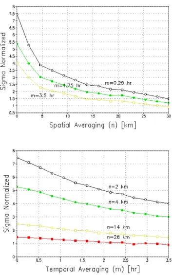
The standard deviation of convective rainfall for this pure radiative convective equilibrium experiment has been computed and the ratio to the sub-domain mean, as a function of the size of the space-time sub-domain, is shown in Fig. 4. Starting from the definition of Islam et al. (1993), the standard deviation of convection is:

^

()

`

1 12

1 1 1

2

» ¼ º «

¬ ª

¦¦¦

Nx i

Ny

j t N

t mn ijt t

Y X mn

C t C N

N N

V (1)

where m and n are the levels of temporal and spatial averaging. Once m and n are fixed, the corresponding number of points N_x, N_y, and N_t will change, as will the number of points averaged in the spatial and temporal directions respectively. In this definition, the value of smn _is the standard deviation of the rainfall process Cmn(t)

ijt ,

simulated at the spatial location (i, j) for a specific level of temporal and spatial averaging, m and n, with respect to C, the mean rainfall. This last value, in the limit for sufficiently large space-time averages, should approach the large scale evaporative flux, and represents a measure of the natural variability of the precipitation process. In this sense, C is not affected by the averaging operator acting on Cijtmn, and is very close to measured values of convective precipitation (for example in the tropics) for the same temporal and spatial averages. Substituting measured values of mean precipitation C in this variance and then normalising smn with them does not change this statistical measure of variability. In this kind of simulation, continuously forced by homogeneous boundary conditions, it may be supposed that the convection itself is horizontally homogeneous in a statistical sense. That is, quantities averaged over space and time domains will not vary appreciably from one sub-domain to the next, provided the sub-sub-domain is large enough. The ratio of the actual space-time sub-domain variance smn of precipitation to the mean C must equal the rate of evaporation.

Figure 4 shows the ratio of the variance of precipitation

to its mean value C for different sized domains (x axis-n: 1= 2km average, 2=2*2 km average, ..) and time scales (y axis: 1= 15 min., 2= 2*15min., ..). Then, this variance is a function of the temporal and spatial average size and may be considered as a space-time volume determined by the space and time scale of the convection itself. To analyse the meaning of this statistical measure, two cross-sections of the normalised standard deviation versus temporal and spatial averaging are shown in Fig. 5, for a few reference values of m and n; in each case, increasing the size of averaging reduces the ratio between the variance and its mean value, reaching a lower limit below which no better value of normalised variance can be found. This is another

Fig. 3. (a) Istantaneous rainfall rate (mm hr–1_{) at the ground; (b) Vertical velocity w (m s}–1_{) for a statistically stable convective atmosphere}

way of expressing the limit that is intrinsic to the averaged space-time volume: this measures the oscillation of convection above a certain averaged value C, beyond which the statistics of convective activity will differ for each volume in the domain. In particular, Fig. 5a shows a cross-section of the standard deviation v. spatial average size for three reference values of temporal averaging; for each curve, the variability depends on the size of averaging. The smaller the spatial averaging size, the larger the standard deviation smn_{for the purely radiative convective equilibrium} experiment. Thus, at statistical equilibrium, the rainfall rate averaged over a large enough area (and/or time) must equal the evaporation from the surface. This effect increases or decreases with the temporal averaging size m. Smaller temporal averaging shifts towards larger rainfall variability, reflecting the oscillation of rainfall rate due to cloud evolution. If the temporal size of averaging is the largest value shown, a limiting value for the rainfall variability is

reached, with values of normalised variability clustered around 1. This value is the least variability shown by the system around 30 km of spatial averaging. The same behaviour decreasing convective variability with increasing temporal average size in a quasi-linear way, depending on the areal average size n for Cijtmn, is shown in Fig. 5b, where smn _{tends to increase with lower values of temporal} averaging.

Hence, the larger the areal domain, the smaller the variance of the modelled data compared to the actual mean (as was expected). However, the importance of this measure is the quantitative comparison between the variance of the possibly forecasted rainfall smn _{to the mean C (a value close to} measured mean values) once the transients of the convective process are gone. Moreover, this kind of oscillation indicates just how noisy the rain rate is in the domain chosen compared to the actual mean. With very similar results, Islam et al. (1993) have shown that smn _{can be a useful tool for selecting} over which area to average rainfall data to avoid non-linearities that affect the field below a certain temporal and spatial average size. Finally, since a different numerical model has been used, without an elastic approximation and with different numerical features, Figs. 4 and 5 represent a quantitative measure of convection and its variability dependent not on the specific numerical model used but rather on the physical mechanisms simulated. The operational utility of this measure is its value in assessing to what extent observations are compatible with the variance of forecasted data.

Numerical experiments on the

orographic effect on atmospheric flow

How does an orographic perturbation affect the dynamics of atmospheric flow? This question, relevant from a dynamic and observational point of view, has been addressed by Queney (1947); Long (1953); Scorer (1949); Klemp and Lilly (1978); Rotunno and Smolarkiewicz (1991). The meteorological phenomena associated with topography have been reviewed in detail in the early work of Queney et al. (1960) and Smith (1979). Among the various effects mentioned, the orographic control of precipitation is associated with both dynamic and thermodynamic mechanisms responsible for rainfall enhancement in the presence of mountains. From an observational point of view, the orographic control of precipitation has been assessed in studies in many parts of the world (Sawyer, 1956; Myers, 1962; Nordo and Hjortnaes, 1966; Chen et al., 1991; Lin, 1993; Jou, 1994; Pandey et al., 1999; Neiman et al., 2002), often under the umbrella of experimental projects such as the Mesoscale Alpine Programme (MAP) in Europe, the

California Landfalling Jets experiment (CALJET) in the

United States and the Taiwan Area Mesoscale Experiment (TAMEX) in Asia, to name recent examples. In Smith (1979) and Lin (2003), a list of different dynamic mechanisms has been proposed to explain orographic rain, while closely spaced convection has been mentioned (Smith, 1979) as a possible cause for stable orographic rain.

However, a general explanation of the dynamics of airflow in connection with the problem of orographic rain is still lacking. In particular, once the correlation between orographic rain and the different dynamic factors controlling it has been assessed, the influence of each factor has to be isolated and studied to identify the extent to which particular mechanisms are responsible for this correlation (Buzzi et al., 1998; Chu and Lin, 2000; Smith et al., 2002; Rotunno and Ferretti, 2002); the dynamic influence of the latent heat release and the local thermodynamic control of precipitation, when moist dynamic processes are considered, has to be analysed. However, the dynamics of convective motions of the airflow with moisture impinging on a mountain barrier is intrinsically non-linear and do not allow the separation of the dynamics of the airflow from the effect of the change of phase of water and latent heat release. Therefore, this study started from an initial general state simulating a field of convective clouds in statistic equilibrium, where an idealised mountain barrier along the y-direction has been introduced; then dynamic factors have been added to perturb this equilibrium state. Given the idealised orography used in this first study, the results are not specific to any particular geographic area. Then, since the dynamic effect caused by the barrier on airflow depends on the scale of the orography, the range of barrier considered has been restricted to small mountains (width ~50 km, after Smith, 1979), for which the Coriolis force can be ignored. In subsequent experiments, Coriolis terms have been included in the equations of motion in a wider domain, to determine the possible influence of

these terms on the dynamics of convective precipitation. These results are not discussed here because they are not relevant to the initial purpose of this paper.

Indeed, for a different BC at the lower boundary in the model, a new equilibrium for convection is reached once the transient due to the numerical adjustment by the flow to the new BC has disappeared. Then, the influence of this new BC on the initial equilibrium state has to be evaluated, theoretically and numerically. In particular, to assess:

l how the simulated flow depends on the height of the mountain. In fact, the first dynamic change produced by the mountain was a variation in convective activity strongly dependent on the height of the mountain at the lower boundary. Moreover, the dynamics of momentum fluxes have been changed by the interaction with the mountain ridge (Eliassen and Palm, 1954).

l whether the BC was suitable for simulating a convective field without introducing non-linearities depends on the complex interaction of the flow with the mountain (e.g. deflection of the flow around the mountain, and other effects deriving from the interaction of ambient characteristics, such as the wind profile, with complex terrain).

l what spatial domain was needed, in the presence of a mountain of a certain width, not to constrain the behaviour of the convective ensemble in an unphysical way that would invalidate the estimate of the convective oscillation.

Several experiments have been run to test particular features relevant to this study.

Firstly, following Durran and Klemp (1983) and Klemp and Lilly (1978), dry experiments have been performed with a stably stratified fluid impinging on mountain barriers of differing heights. The different values for parameters in the

Table 1. Parameters of mountain wave experiments

Experiment parameters LH NLNH Boulder Windstorm

hm (m) 1 503 2000

a (m) 10000 2000 10000

D_{x (m) 2000 400 1000}

D_{y (m) 250 125 200}

L (domain width, km) 576 460 512

H (domain depth, km) 24 24 28

D_{t 20 10 2.5}

Dt _{5 1 2.5}

Reyleigh damping coeff. (1/s) 0.0015 0.0025 n.a.

Height damper starts (km) 12 9 n.a.

4th

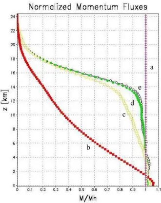
initial mountain experiment are shown in Table 1. Three types of simulation have been run, depending on the type of flow and of the solution that the analytical (and numerical) equation displays. Each of these experiments, well known in the literature, checks the correctness of the numerical solution against the analytical one and, therefore, the ability of the numerical model to reproduce them. Linear and hydrostatic, non-linear and non-hydrostatic experiments have been run, depending on the width and amplitude of the mountain (quantities a and h_m in Table 1). In the first case, flow around the mountain was hydrostatic with a low Froude number (Fr«1), while in the second case, the dynamics of the flow were non-hydrostatic (Fr=0.5) with lee wave separation with flow over and around the mountain. In the linear case, the correct vertical momentum flux propagation has been verified. In the mountain wave problem, it is assumed that all the vertical fluxes vanish at the lower boundary, as well as the normal velocities. Figure 6 shows the vertical momentum flux normalised with the hydrostatic linearised value for the linear mountain case; the analytical value (line a) of the horizontal momentum can be computed explicitly from:

dx

w

p

M

’ ’

³

f_f

(wirh p´ and w´ being the pressure and vertical velocity perturbation, respectively) as the drag per unit length in the case of a bell-shaped mountain (Smith, 1979):

2 0

4 NUhm D S U

where r₀ is the density, N is the static stability at ground level, U is the uniform wind speed and hm is the amplitude of the mountain. The analytical value of the vertical profile of horizontal momentum transport by gravity wave processes has to be compared with the vertical profiles obtained by the numerical integration of the linear wave equation for the bell-shaped mountain case, where curves (b), (c), (d) and (e) in Fig. 6 are profiles obtained at different times and scaled with the same analytical value. Given this normalisation, the analytical value corresponds to a value of unity, while the simulated profiles are almost equal to unity at the surface and very close to it at later times (curve (e) below the Raleigh damping layer (15.5 km)). This sponge layer absorbing waves above the tropopause has been added to the numerical scheme of the ARPS model to absorb the waves excited by the orographic perturbation so that they will have negligible amplitude when they reach the top of it. This ensures that reflections of energy are minimised and a correct flux of vertical momentum results. This absorber of waves was needed in the experiment because the BC changes the flow and convective activity, since convective motion is able to produce gravity waves even without mean wind, as is implied by expression for D for the horizontal momentum for these dry mountain wave experiments. The effect of the sponge layer is that the numerical solution provided by the model absorbs waves without changing the solution appreciably and, after the initial adjustment, resolves the flow with a very high degree of approximation. This experiment shows that the mountain introduces, in the wind and thermodynamic fields, a dynamic perturbation which depends strongly on the height of the ridge; this choice affects both linear and non-linear perturbation of the wind field. Therefore, given the size of the domain in the vertical (20 km) and its resolution in space and time, the height of the mountain (corresponding to the amplitude h_m in the wave equation, see Smith, 1979) had to be limited to 500 m.

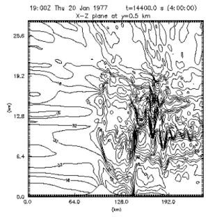
Because the influence of moisture can be introduced through its effect on the vertical stability of the atmosphere changing the sounding applied as an initial condition to the experiment, the last test has been the down-slope windstorm case of a severe windstorm on the lee side of the Rocky Mountains in the 1970s and subsequently studied by Klemp and Lilly (1975); Peltier and Clark, (1979); Klemp and Durran, (1983). The wind field is shown in Figs. 7 and 8 for 2.5 and 4 hours of the simulated storm. Corresponding to

Fig. 6. Vertical flux for the horizontal momentum normalised for different time. From curve (a) normalised value M, (b), (c), (d) and (e) simulated value with increasing time.

a

b

c d

these strong winds (80–90 m s–1_{), both at the surface and}

aloft, a hydraulic jump developed, with a front reversal resulting in flow overturning and strong mixing. This corresponds to the oscillation and breaking of the waves along the lee slope of the mountain (Front Range), accompanied by strong horizontal winds. This wave activity resulted in heavy precipitation due to the strong oscillation above the mountain. This last case has been simulated here to check the ability of the ARPS model to reproduce the dynamics over a mountain using a simplified terrain in

comparison with the same experiment using a realistic terrain profile (see Peltier and Clark, 1979). The dynamic features of the down-slope flow are consistent with the experiment run with realistic terrain, so that, from a dynamic point of view, the impact of a realistic terrain is of higher order than that of the simplified orography (ridge along y direction) and the other terrain parameters considered here. Following Eliassen and Palm (1954), the flux of horizontal momentum is typical of mountain perturbation. Incorrect reflection of the vertical momentum flux can change the dynamic balance for the flow and, hence, the choice of the absorbing layer. Figure 10a and b shows gravity waves excited by the convective activity around the ridge, and travelling through all domains in the case of the 500 m ridge. A negative and positive pattern of horizontal velocity perturbation is developing in the vertical direction and dispersing the amplitude of the wave through the atmosphere. It is the gravity wave’s field that produces heavy precipitation due to the strong oscillation of the flow above and around the mountain.

Orographic effect on rainfall

variability

Having established how the simulation depends on the BC chosen for the energy and velocity fields, the orographic effect on the convective activity must be evaluated. The second part of the predictability experiment enlarged the domain of simulation, to ensure that the statistics of the physically meaningful quantities at radiative-convective equilibrium would be independent of the size of the domain with the mountain. This was done by running the model with the physical parameters used during the flat experiment and then observing the various scales of adjustment on which convection reaches equilibrium. It was stressed earlier that convective activity in the present experiment depends upon surface fluxes, radiation and large-scale forcing. In most of the case studies simulated within the EFFS project, large-scale forcing and orography may trigger convective cells. To ensure that the simulation and subsequent statistics account for all the processes that determine both the convective cells and their organisation, a domain large enough to contain all the spatial- and time-scales that determine the equilibrium state must be considered; for flat BCs, such a domain was shown to be less than the dimension of the previous experiment (66 × 66 grid points). Nevertheless, in this last experiment with orography, the horizontal domain was enlarged to 95 × 95 horizontal grid points, to accommodate the dynamic effect of the width of a bell-shaped mountain, 60 km wide and from 500–1000 m high. Given the periodic BCs for the horizontal domain, the

Fig. 7. Horizontal velocity field u at 2 hrs. for the down-slope windstorm with idealised orography

ridge width is a constraint from a dynamic point of view because of the infinite domain considered. The size chosen for this experiment allows the typical time-scale of convective motions (N–1_{) to be much less than the travelling}

time-scale for waves from one ridge to another. This choice considers that the mountain height h is small compared to the mountain width L_{, so that the terrain feature may be}

considered to be rather gentle (h/L_{), at least for the 500 m}

ridge; this produces small disturbances that can be treated with the BCs and spatial resolution adopted within the domain considered. The adjustment of potential temperature, relative humidity, moist static energy and the energy balance have been evaluated on time-scales of tenths of days to let the numerical simulation reach a stable state. Despite these considerations, several non-linear interactions are possible between disturbances of mountain height h and other length scales in a continuously moist stratified atmosphere, if a mean wind or shear are included in the simulation. Moreover, once the Rossby number for these waves has been considered (2pN/f) possible rotational effects on the flow have been addressed by including Coriolis terms in the equations. With this domain size, the first result showed no visible rotation effect on the dynamics of flow for a time-scale extending beyond the temporal range of interest (10 days).

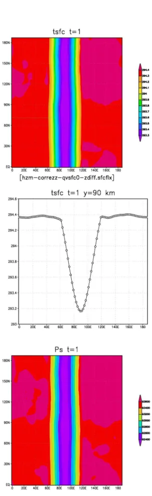
Because of the moist dynamic used, the main effect on the thermodynamics of the flow is due to the consistent anomaly in potential temperature (equal to absolute temperature at the surface) because of the change in pressure when the parcel is lifted above the mountain. The consequent surface temperature variation ranges from 1.2 K at the mountain peak for the 500 m ridge to more than 2 K for the 1000 m ridge. Figure 9a and b shows the anomaly in pressure and potential temperature for the 500 m. mountain. This anomaly is only part of the thermodynamic effect on atmospheric flow due to the mountain and reflects the mechanical lifting of the atmospheric parcel above the mountain ridge. For a hill 500 m high, the main orographic effect on flow is the enhancement of convective activity because of the anomaly on the condensation and formation of rainfall, which interacts with the cold pool mechanism which produces convection (Fig. 3), as studied by Tompkins (2001). However, this will not be true for the 1000 m ridge mountain, where the temperature anomaly is much higher and leads to more complex flow dynamics. This first study has focused particularly on the variability of the convective activity due to this orographic temperature anomaly.

Three experiments have been run on a domain of 95 × 95 × 41 grid points with an horizontal resolution of 2 km, unchanged from the previous experiment because both the horizontal and the vertical resolution are adequate to

resolve the eddies and the turbulent cascade with this model

setting (not shown). Figure 10a and b compare the effect of a 500 m ridge on the convective activity for a horizontal velocity field with the 2-D simulations. The mountain perturbation is connected to a convective wave, excited by

the surface anomaly in temperature and modulated by the height of the mountain ridge. Figure 10b shows the mountain effect amplified, when an anvil has developed over the ridge and cumulus clouds are spread over the domain by the convective perturbation of the flow. The convective activity

Fig. 10 (a) Horizontal velocity in a x–z slice, with a bell-shaped mountain of 500 m. (b) Horizontal velocity in a x–z slice, with a bell-shaped mountain of 500 m; same time as (a) but with different y position

(a)

in these experiments is balanced not only on the cumulus time-scale, reflected by the average rate of rainfall but it is also in equilibrium on an atmospheric moisture time-scale, reflected by the vertical relative humidity profile attained after several tenths of days (not shown). The oscillation of this balance is amplified by the time-scale for field storage (0.5 hr ~ cumulus cloud lifetime). Indeed, to appreciate small variations in rainfall rate and dynamic variables, a time storage of about 15 minutes would be sensitive to most changes in convective activity. However, in consideration of the time for atmospheric humidity to equilibrate (several tenths of days), this is unrealistic; also, for this range of simulation, it would result in an unmanageable amount of data. Therefore, for the storage of variables, the average lifetime of cumulus clouds was chosen.

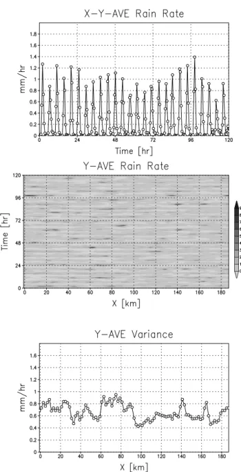
The upper panel of Fig. 11 compares the horizontally averaged rain rate versus time for a simulation run without orography with an equivalent run with the mountain simulations. The horizontally averaged rainfall rate indicates how close the system is to equilibrium; a continuous and regular rainfall rate profile exhibits oscillations corresponding to changes in the relative humidity horizontally averaged vertical profile. Other convective variables, namely cloud mass flux and potential temperature profile, have two maxima, corresponding to shallow and deep convecting clouds, respectively. The middle panel in Fig. 11 shows the Hövmoller diagram for the y-averaged rainfall rate, the oscillation for which is distributed all over the domain, with maxima not corresponding to any preferred direction. If the lower panel for Fig. 11 is analysed along the y-direction, any appreciable difference in rainfall variance can be detected once equilibrium is attained.

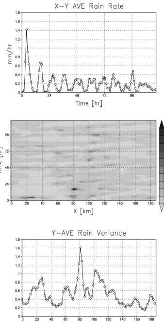
Figure 12 shows the rain rate versus time and its variance in the case of a convective atmosphere where the mountain is a 500 m barrier in the y-direction. This experiment is of a simple orographic interaction as discussed above. The upper panel of Fig. 12 indicates that, after an initial transient, the averaged rainfall rate on the whole domain has been reduced by the presence of the mountain ridge. The mountain enhances the convective activity above the mountain ridge, although it does not inhibit the convective activity around the ridge, as shown in the middle panel of the same figure, which is the Hövmoller diagram for the y-averaged rainfall rate. In this case, the variance peaks well above the former equilibrium value (lower panel of Fig. 12), despite the fact that the convective activity is suddenly reduced when the mountain is introduced in the domain (before this the periodic boundary condition allowed cumulus cloud to span freely all over the domain).

The effect of the orographic barrier can be seen more clearly with a mountain ridge 1000 m high. Not only a sharp

gradient in convective activity but also a strong change of the rain variance is expected. The upper panel of Fig. 13 shows the rain rate versus time averaged over the entire horizontal domain while the distribution in time versus space of the same quantity is shown in the middle panel. The effect of reduction in the rainfall intensity and the increased variance over and around the mountain ridge are shown in the lower panel. The perturbation caused by the mountain ridge concentrates the convective activity and enhances it around the mountain because of the potential temperature

297 anomaly. As can be seen, particularly for the case of the

1000 m mountain, the variance in rainfall rate variance is higher upstream and downstream of the mountain but lower just above the peak of the ridge. As emphasised previously, the dynamic impact on the atmospheric flow of the 1000 m ridge differs from that of the 500 m ridge, and seems to confine the gravity waves excited by convection.

Conclusions

The effect of orography on convective rainfall variability with respect to the initial value problem has been approached differently from that adopted during the EFFS project. Conventionally, this problem has been addressed through case studies on initial value problems, the statistical findings of which cannot be generalised because of their dependence on the initial conditions. This is a first attempt to link the problem of convection simulation with that of simulating the dynamics for orographic rainfall.

Fig. 12. Rain rate for convection with a barrier of 500 m at 90 km along the x direction. Upper panel: x–y averaged rain rate with total and variance, middle panel: Hövmoller diagram of the y averaged rain rate; lower panel: variance of the Y averaged rain rate.

The first requirement has been to find a dynamic and statistically stable numerical state from which to start an experiment to compute the convective variance for a flat domain independent of the initial conditions imposed on the system. The experiment studied an idealised environment using the simplest mechanism able to produce convection, as in a tropical atmosphere or in sunny weather conditions at mid-latitudes. Following Islam et al. (1993), the convective variance for the field of deep and shallow clouds resulting from convective activity at equilibrium has been computed; notwithstanding the different numerical model used and conditions applied, results were similar to those in the Islam et al. study. This concerns the intrinsic variability of a convective rain field simulated by numerical non-hydrostatic models forced only by surface fluxes of heat and moisture; these equilibrate, in a statistical energy equilibrium of moist convection, with the radiative cooling rate. Radiative cooling reproduces the interaction of the convective cloud field with the radiative field and the large-scale forcing caused by the large-large-scale ascent of air. This simulated value of convective variability for rainfall identifies the variability corresponding to averaged values for convective rainfall at the level of confidence specified. An operational application of this statistical evaluation is that, for a specified level of confidence required for forecast evaluation, it can be used to assess the level of variability for averaged measured values of convective rainfall.

After these experiments had been completed, numerical aspects introduced by an orographic perturbation in the resultant numerical and physical model were tested to assess its ability to reproduce the effect of an orographic perturbation applied at the lower boundary of the model. In particular, a suitable domain for a certain height for the mountain ridge level has been selected; this has been positioned along the y direction with an absorbing layer at the tropopause to study, firstly, a simple orographic perturbation without complex interactions with the atmospheric moist flow. The initial domain has been enlarged from the flat experiments to avoid physical constraints on the development of convection and convective activity has been measured, statistically, with a mountain ridge of different heights. Early results show an intensification of convective rainfall around and above the mountain ridge, with a higher rainfall rate corresponding to a higher barrier. This effect is associated with the potential temperature anomaly deriving from the difference of the pressure field along the mountain profile. The quantitative value of variance for convection in these cases results from different dynamic mechanisms, but there is no doubt that convective activity is modified strongly by the presence of the mountain ridge and, specifically, is enhanced by it.

The 1000 m ridge experiment shows an enhancement of orographic rainfall, although with more complex dynamics, involving gravity waves and the mountain ridge. The existence of these gravity wave modulations in the rainfall variability around and above the mountain barrier makes it difficult to take account of rainfall variance once very clustered data in space and time are considered. If raingauge data are considered, they reflect the gravity wave modulation and their meaning, on a small spatial and temporal scale, is limited by this noisy interaction with the convective waves. The statistical evaluation given is unable to filter out this modulation but is a first step to account for different effects on rainfall variability.

The aim of the first part of the study has been to show the strength of the effect of dynamic and thermo-dynamic factors controlling convection in a simple case of orographic forcing. Specifically, an attempt was made to account for different effects controlling convective activity when a mountain ridge perturbs a statistically stable convective system. Although it reaches a thermo-dynamic and dynamic equilibrium, the spatial and temporal scales of this equilibrium differ from the unperturbed case. This leads to different convective activity and changes the convective rainfall variability. A better approach to accounting for rainfall variability is to separate the mechanical effect due to perturbation by the mountain from other thermo-dynamic effects on the flow. Although in the EFFS project, meteorological aspects connected with the hydrology and particularly with the flood problem have been considered, some dynamic issues deserve further investigation. The first generalisation might be the introduction of a different orographic lower boundary (and even realistic orography) in the chosen domain, as well as a more complex dynamic environment, with mean wind and vertical shear to organise convection on different scales.

References

Arakawa, A. and Shubert, W.H., 1974. Interaction of a cumulus cloud ensemble with the large-scale environment. I. J. Atmos. Sci.,31, 674–701.

Buzzi, A., Tartaglione, N. and Malguzzi, P., 1998. Numerical simulations of the 1994 Piedmont flood: role of orography and moist processes. Mon. Weather Rev., 126, 2369–2383. Chen, F., Warner, T.T. and Manning, K., 2001. Sensitivity of

orographic moist convection to landscape variability: a study of the Buffalo Creek, Colorado, flash flood case of 1996. J. Atmos. Sci.58, 3204–3223.

Durran, D.R. and Klemp, J.B., 1983. A compressible model for the simulation of moist mountain waves. Mon. Weather Rev., 111, 2341–2361.

Emanuel, K. A., Neelin, J.D. and Bretherton, C.S., 1994. On large

scale circulation in convecting atmospheres. Quart. J. Roy. Meteorol. Soc., 120, 1111–1143.

Enthekabi, D., Asrar, G.R., Betts, A.K., Beven, K.J., Bras, R.L., Duff y, C.J., Dunne, T., Koster, R.D., Lettenmaier, D.P., McLaughlin, D.B., Shuttleworth, W.J., van Genuchten, M.T., Wei, M. and Wood, E.F., 1999. An agenda for land surface hydrology research and a call for the Second International Hydrological Decade. Bull. Amer. Meteorol. Soc., 80, 2043– 2058.

Islam, S., Bras, R.L. and Emanuel, K.A., 1993. Predictability of mesoscale rainfall in the tropics. J. Appl. Meteorol., 32, 297– 310.

Kaufmann, P., Schubiger, F. and Binder, P., 2003. Precipitation forecasting by a mesoscale numerical weather prediction (NWP) model: eight years of experience. Hydrol. Earth Syst. Sci.,7, 812–832.

Klemp, J.B. and Durran, D.R., 1983. An upper boundary condition permitting internal gravity wave radiation in numerical mesoscale models. Mon. Weather Rev. 111, 430–444.

Klemp, J.B. and Lilly, D.K., 1975. The dynamics of wave-induced downslope windstorm. J. Atmos. Sci..32, 320–339.

Klemp, J.B. and Lilly, D.K., 1978. Numerical simulation of hydrostatic mountain waves. J. Atmos. Sci.,35, 78–107. Long, R.R., 1953. Some aspects of the flow of stratified fluids, I

a theoretical investigation. Tellus5, 42–58.

Orlanski, I., 1975. Rational subdivision of scales for atmospheric processes. Bull. Amer. Meteorol. Soc., 56, 527–530.

Peltier, W.R. and Clark, T.L., 1979. The evolution and stability of finite amplitude mountain waves. Part II: surface wave drag and severe downslope windstorms. J. Atmos. Sci.,37, 2122– 2125.

Queney, P., 1947. Theory of perturbations in stratified currents with applications to airflow over mountain barriers. Misc. Report No 23, Dept. of Meteorology, Univ. of Chicago, USA.

Richard, E., Cosma, S., Benoit, R., Binder, P., Buzzi, A. and Kaufmann, P., 2003. Intercomparison of mesoscale meteorological models for precipitation forecasting. Hydrol. Earth Syst. Sci.,7, 799–811.

Robe, F.R. and Emanuel, K.A., 1996. Moist convective scaling: inferences from three-dimensional cloud ensemble simulations.

J. Atmos. Sci., 53, 3265–3265.

Rotunno, R. and Smolarkiewicz, P.K., 1991. Further results on lee vortices in low-Froude-number flow. J. Atmos. Sci., 48, 2204–2211.

Sawyer, J.S., 1956. The physical and dynamical problems of orographic rain. Weather, 11, 375–381.

Scorer, R.S., 1949. Theory of lee waves of mountains. Quart. J. Roy. Meteorol. Soc., 75, 41–56.

Smith, R.B., 1979. The influence of mountains on the atmosphere.

Adv. Geophys.,21, 87–230.

Smith, R.B., Skubis, S., Doyle, J.D., Broad, A.S., Kiemle, C. and Volker, H., 2002. Mountain waves over Mont Blanc: influence of a stagnant boundary layer. J. Atmos. Sci.,59, 2073–2092. Tompkins, A.M., 2001. Organization of tropical convection in low

vertical wind shears: the role of coldpools. J. Atmos. Sci., 58, 1650–1672.

Tompkins, A.M. and Craig, G.C., 1998a. Radiative-convective equilibrium in a three-dimensional cloud ensemble model.

Quart. J. Roy. Meteorol. Soc., 124, 2073–2097.

Tompkins, A.M. and Craig, G.C., 1998b. Time-scales of adjustment to radiative-convective equilibrium in the tropical atmosphere.

Quart. J. Roy. Meteorol. Soc., 124, 2693–2713.