www.biogeosciences.net/9/217/2012/ doi:10.5194/bg-9-217-2012
© Author(s) 2012. CC Attribution 3.0 License.
Biogeosciences
Seasonal and inter-annual variability of plankton chlorophyll and
primary production in the Mediterranean Sea:
a modelling approach
P. Lazzari1, C. Solidoro1, V. Ibello1,*, S. Salon1, A. Teruzzi1, K. B´eranger2, S. Colella3, and A. Crise1
1Istituto Nazionale di Oceanografia e di Geofisica Sperimentale – OGS, Trieste, Italy 2Ecole Nationale Sup´erieure de Techniques Avanc´ees, ENSTA ParisTech, Palaiseau, France´ 3Centro Nazionale delle Ricerche, CNR ISAC UOS, Roma, Italy
*now at: Institute of Marine Sciences, Middle East Technical University, Erdemli, Turkey Correspondence to:P. Lazzari ([email protected])
Received: 3 May 2011 – Published in Biogeosciences Discuss.: 1 June 2011
Revised: 16 November 2011 – Accepted: 14 December 2011 – Published: 11 January 2012
Abstract. This study presents a model of chlorophyll and
primary production in the pelagic Mediterranean Sea. A 3-D-biogeochemical model (OPATM-BFM) was adopted to explore specific system characteristics and quantify dynam-ics of key biogeochemical variables over a 6 yr period, from 1999 to 2004. We show that, on a basin scale, the Mediter-ranean Sea is characterised by a high degree of spatial and temporal variability in terms of primary production and chlorophyll concentrations. On a spatial scale, important horizontal and vertical gradients have been observed. Ac-cording to the simulations over a 6 yr period, the devel-oped model correctly simulated the climatological features of deep chlorophyll maxima and chlorophyll west-east gra-dients, as well as the seasonal variability in the main off-shore regions that were studied. The integrated net primary production highlights north-south gradients that differ from surface net primary production gradients and illustrates the importance of resolving spatial and temporal variations to calculate basin-wide budgets and their variability. Accord-ing to the model, the western Mediterranean, in particular the Alboran Sea, can be considered mesotrophic, whereas the eastern Mediterranean is oligotrophic. During summer stratified period, notable differences between surface net pri-mary production variability and the corresponding vertically integrated production rates have been identified, suggesting that care must be taken when inferring productivity in such systems from satellite observations alone. Finally, specific simulations that were designed to explore the role of external fluxes and light penetration were performed. The subsequent results show that the effects of atmospheric and terrestrial
nutrient loads on the total integrated net primary production account for less than 5 % of the its annual value, whereas an increase of 30 % in the light extinction factor impacts pri-mary production by approximately 10 %.
1 Introduction
The qualitative and quantitative dynamics of biogeochemical properties in the open ocean are not well understood despite a growing awareness of their importance to ecosystem func-tioning and related goods and services on a planetary scale.
Monitoring programs are currently widespread in coastal areas but seldom cover open ocean waters, and they are prin-cipally devoted to the measurement of physical variables. Remote sensing observations provide valuable knowledge but primarily at the sea surface level. Research cruises en-able scientists to explore ocean interior; however, these are limited to a few transects per year and often have inadequate sampling rates at seasonal or inter-annual time scales. Bio-geochemical floats and gliders are not currently used in sus-tained observational programs.
The use of validated models to reconstruct and explore the spatial and temporal dynamics of a property that can-not be readily measured at high frequency is already quite common in other fields, such as hydrology, and is now being increasingly applied in global ocean studies as well (Sarmiento and Gruber, 2006; Follows et al., 2007; Le Qu´er´e et al., 2010). This is relevant despite the fact that, in these cases, it may not be possible to use strictly validated mod-els (Arhonditsis and Brett, 2004). In principle, by optimally merging theoretical knowledge that is coded into a model with available experimental observations, data assimilation would provide insight into system functioning and properties where experimental observations are sparse.
In this article, we explore the spatial and temporal vari-ability of chlorophyll concentrations and plankton primary production rates in the epipelagic open ocean waters of the Mediterranean Sea (MS hereafter) with a state-of-the-art nu-merical model that is constrained by satellite data. Model re-sults provide useful information for developing a better un-derstanding of MS trophodynamics and 3-D climatological descriptions of biogeochemical properties that could be use-ful as evidence-based support for regulations that are aimed at marine protection and conservation (such as the Marine Strategy Framework Directive) or as a comparison point for future studies and cross-site analyses. Annual budgets and temporal variability of chlorophyll concentrations and net primary production (NPP hereafter) are presented for differ-ent MS sub-basins and compared to previous studies.
2 Methods
2.1 The Mediterranean Sea
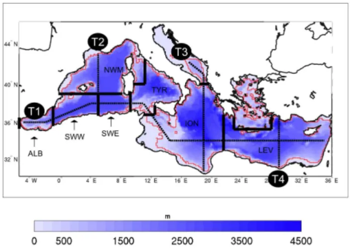
The MS is the largest semi-enclosed basin in the world. The Strait of Sicily separates the western and eastern sub-basins, which are shifted latitudinally, and can, in turn, be subdivided into several regional seas based on bathymetric and morpho-logical considerations (Fig. 1). Physical processes create a dynamic and complex system in which mesoscale, thermoha-line and wind driven circulations interact at different scales, resulting in a dominant west to east surface transport partially compensated by east to west transport at intermediate depths (Pinardi and Masetti, 2000).
The MS has long been considered one of the most olig-otrophic areas in the world (Azov, 1991). Low primary pro-duction annual budgets have been estimated by several stud-ies based on in situ measurements (i.e., Sournia, 1973; Ro-barts et al., 1996; Moutin and Raimbault, 2002). Ocean colour satellite analysis clearly indicates a decreasing west-east trophic gradient in productivity (Bosc et al., 2004; Volpe et al., 2007; Barale et al., 2008; D’Ortenzio and Ribera d’Alcal`a, 2009), confirmed by (sparse) in situ measurements (Turley et al., 2000). Model analysis has indicated that this gradient is created by the superposition of physical dynamic
Fig. 1.Map of Mediterranean Sea bathymetry, with a-priori defined regions (delimited by solid black lines) and T1, T2, T3 and T4 tran-sects (dashed black lines). ALB = Alboran Sea, SWW = South Western Mediterranean Sea (western side), SWE = South West-ern Mediterranean Sea (eastWest-ern side), NWM = North WestWest-ern Mediterranean Sea, TYR = Tyrrhenian Sea, ION = Ionian Sea, LEV = Levantine basin. Red line indicates shallow water limits (depth<200 m).
features and asymmetric distributions of nutrient sources and is maintained by biological pump activity (Crise et al., 1999, 2001). Satellite estimations have also demonstrated an anal-ogous meridional trophic gradient from the north to the south (Siokou-Frangou et al., 2010). These spatial patterns are reflected in the location of the deep chlorophyll maximum (DCM), which is a quasi-permanent structure, except during the winter mixing period, characterised by a zonal gradient in terms of depth (shallower in the west and deeper in the east; Crispi et al., 1999; Siokou-Frangou et al., 2010). De-spite its oligotrophic features, the MS maintains high levels of biodiversity (Bianchi and Morri, 2000; Coll et al., 2010) and some hot spots for fisheries (Caddy et al., 1995).
The lack of spatial-temporal coverage of in situ measure-ments does not allow for a direct estimate of the annual bud-get and temporal variability of NPP, except for specific sites, such as the DYFAMED station (Marty and Chiav´erini, 2002) and other Long Term Ecological Research stations (Pugnetti et al., 2006). Therefore, there are large uncertainties in present estimates of NPP at the basin scale due to the sparcity of available observations (Sournia, 1973).
2.2 The numerical model
coupled in an operational tool for studying MS biogeochem-istry (Lazzari et al., 2010) and are applied here, with several modifications.
The model solves a system of partial differential equations describing the temporal evolution of the concentration of a tracercias:
∂ci
∂t =A+D
v+S+R,
(1) whereArepresents the advection term,Dvthe vertical diffu-sion term,Sthe sinking term (only for particulates) and the reaction termRbiological and chemical processes.
2.2.1 The transport terms
The physical dynamics that are coupled with biogeochemical processes are pre-computed by a high resolution ocean gen-eral circulation model (OGCM MED16). This circulation model supplies temporal evolution fields of horizontal and vertical current velocities; vertical eddy diffusivity; poten-tial temperature; salinity, in addition to surface data for solar shortwave irradiance and wind stress. The associated trans-port terms (advectionA, vertical diffusion Dv and sinking
S, see Eq. (1)) are integrated off-line by a modified version of the OPA tracer model, version 8.1, on parallel machines via the method of domain decomposition, according to the equations presented in Appendix A. The off-line integration scheme implies that concentrations of biogeochemical prop-erties (other than salt) do not significantly affect circulation, which is a reasonably safe assumption in the MS.
The dynamical model is called MED16, and is a regional configuration of the primitive-equation rigid-lid numerical model Ocean PArallel (OPA) (Madec et al., 1997) for the MS (B´eranger et al., 2005). Its horizontal resolution is 1/16◦ in longitude and 1/16◦cos(φ) in latitude (φ is the latitude), which corresponds to about 6 km, with 43 vertical levels on a stretched grid with layer thickness increasing from 6 m at the surface to 200 m at the bottom. The initial state of the simulation is the climatology MODB4 from Brankart and Brasseur (1998) in the MS and the climatology of Reynaud et al. (1998) in the Atlantic Ocean. A buffer zone is applied in the Atlantic domain. The horizontal eddy momentum and tracer diffusivity are parameterised by a bi-harmonic opera-tor (coefficient equal to−3×10⁹m4s−2). The vertical dif-fusivity for tracers and momentum is modeled with the Tur-bulent Kinetic Energy closure scheme proposed by Blanke and Delecluse (1993). In case of vertical static instabilities, the vertical diffusivity is increased to a threshold value of 1 m2s−1. The mixed layer depth is diagnosed as the depth at which the vertical diffusivity coefficient corresponds to the threshold value taking care of vertical static instability. Starting from rest, the MED16 model was forced by the rean-alyzed fields from ERA40 (Uppala et al., 2005) from January 1989 to February 1998 period, and then by the ECMWF anal-yses from March 1998 to 2006. The net climatic heat fluxes,
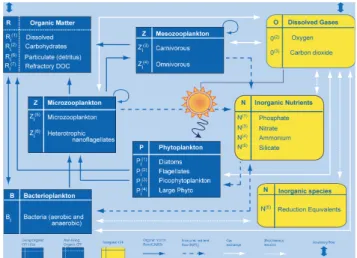
Fig. 2. Compartments and processes in the Biogeochemical Flux Model. Scheme modified from Vichi et al. (2007a), Copyright ©2006, with permission from Elsevier.
the Reynolds SST, the freshwater E-P flux and the wind stress are as described in Barnier (1998). Between March 1998 and October 2000, the resolution of ECMWF was 60 km, then increased to 40 km from November 2000 to 2006. The stud-ied period (1999–2004) has been validated by B´eranger et al. (2009, 2010) who showed that the MED16 model is able to reproduce winter convection events in the main areas of the MS.
2.2.2 The biogeochemical model
The biogeochemical model (corresponding to the reaction termRin Eq. (1)) is a modified version of the Biogeochem-ical Flux Model, BFM. This model describes dissolved and particulate organic and inorganic components as functions of temperature, salinity, irradiance level and other biogeochem-ical properties (Fig. 2). This model’s complexity has been chosen considering the need to describe energy and mate-rial fluxes through both “classical food chain” and “micro-bial food web” pathways (Thingstad and Rassoulzadegan, 1995), and to take into account co-occurring effects of multi-nutrient interactions. Both of these factors are very important in the MS, wherein microbial activity fuels the trophodynam-ics of a large part of the system for much of the year and both phosphorus and nitrogen can play limiting roles (Krom et al., 1991; B´ethoux et al., 1998).
A detailed description of the BFM is given in Vichi et al. (2007a). In the version adopted here we modified the chlorophyll synthesis parameterisation, because several tests have shown that surface chlorophyll and NPP levels in the MS oligotrophic areas were higher than those identified via SeaWiFS satellite estimations and in situ primary production measurements. The introduction of a multi-nutrient (nitro-gen and phosphorus) limitation in the chlorophyll synthesis equation has improved this situation. Furthermore, we have constrained the model dynamics with a satellite-based light extinction coefficient.
Following Geider et al. (1997), the BFM parameterisa-tion describes gross primary producparameterisa-tion (gpp) in terms of PAR, temperature (both linearly interpolated in time from the MED16 outputs), carbon quota in plankton cells (C), chlorophyll content per unit of carbon biomass (θ), and sil-icate concentrations in the case of diatoms. In the previous BFM version, chlorophyll synthesis rate was proportional to the carbon synthesis rate which, in turn, is limited by inter-nal nitrogen quotas. This formulation implies (as our tests indicated) that, in phosphorous-limited conditions the syn-thesis of carbon and chlorophyll are overestimated. In the BFM version used in this study, we included the effect of phosphorus limitation on carbon synthesis kinetics using a multi-nutrient limitation rule as proposed by Flynn (2001) involving both nitrogen and phosphorous and following the Liebig rule.
The revised formulation reads as shown in Appendix B, and the complete list of parameters that were used in our ex-periments is reported in the Supplement (part 2).
2.2.3 Constraining the model using satellite
observations
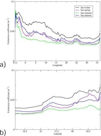
Several test simulations have revealed that standard formu-lations for light extinction factors based on water absorption and plankton self-shading (Riley, 1975) do not adequately describe the observed light attenuation along the water col-umn and the spatial differences in DCM depth between MS sub-basins. We have assumed that the water optical proper-ties were not of the Yerlov “case I” type, owing to the pres-ence of “yellow substances” (CDOM) that can increase the water’s absorption coefficient (Morel and Gentili, 2009). Be-cause the dynamics of such substances cannot be modelled, we used a light extinction coefficient (k) that was derived from satellite observations. As a consequence, we implicitly included, albeit empirically, the effects of all dissolved and particulate matter. As shown in Fig. 3,kis space- and time-dependent: higher values are observed during the winter in the western Mediterranean area. The light model that was used to evaluate the photosynthetic available irradianceI (z)
at different depths (z) is based on the Lambert-Beer formu-lation:
I (z)=I (zo)e−k(x,y,z,t )z (2)
Fig. 3. Satellite extinction factor used in model simulations, zonal averages (upper panel) and meridional averages (lower panel), data provided by GOS-ISAC-CNR.
k(x,y,z,t)=ksat(x,y,t ), (3)
whereI (z0)is the irradiance at the surface level, andx,y and t are longitude, latitude and time, respectively. The light attenuation term (k) is derived from SeaWiFS data (ksat) adopting the diffuse attenuation coefficient at 490 nm (K490; see the web reference at oceancolor.gsfc.nas.gov);
ksat consists of seasonal climatological measurements over the 1998–2004 period, which were spatially interpolated onto the model grid with a 5-day temporal frequency.
It might be argued that, strictly speaking, the use of surface
ksatto determinekfor the whole water column is not correct. However, the absolute error due to uncertainty in the rate of decay ofkwith depth is larger than the error due to the use ofksat. Further, sensitivity analysis of the effect of varyingk on the NPP is presented here.
2.2.4 The initial and boundary conditions in the
numerical experiments
using vertical profiles from a retrospective reanalysis per-formed during the MFSTEP project using the MEDAR-MEDATLAS 2002 data set (Crise et al., 2003). The extracted data include measurements of dissolved oxygen (from 1948 to 2002), nitrate (from 1987 to 2002), phosphate (from 1987 to 2002) and silicate (1987 to 2002). A vertical nutrient pro-file was assigned to each of the eleven regions, as reported in Crise et al. (2003). The other biogeochemical state vari-ables were homogeneously initialised in the photic layer (0– 200 m) according to the standard BFM values and with lower values in the deeper layers. A smoothing algorithm was ap-plied to manage the discontinuities between the different sub-domains.
A Newtonian dumping (DN) term regulates the Atlantic buffer zone that is outside of the Strait of Gibraltar:
DN=1
τ
ciD−cti (4)
whereτ is the time scale of the relaxation, and the tracer con-centrationci is relaxed to the seasonally varying value cDi , which is derived from climatological MEDAR-MEDATLAS data (phosphate, nitrate, silicate, dissolved oxygen) mea-sured outside Gibraltar.
Atmospheric deposition rates of inorganic nitrogen and phosphorus were set according to the synthesis proposed by Ribera d’Alcal`a et al. (2003) and based on measurements of field data (L¨oye-Pilot et al., 1990; Guerzoni et al., 1999; Herut and Krom, 1996; Cornell et al., 1995; Bergametti et al., 1992). No distinction was made between dry and wet depositions, and all of the deposited nutrients were con-sidered to be bio-available. Atmospheric deposition rates of nitrate and phosphate were assumed to be constant dur-ing the year, albeit with different values for the western (580 Kt N yr−1and 16 Kt P yr−1) and eastern (558 Kt N yr−1 and 21 Kt P yr−1) sub-basins. The rates were calculated by averaging the “low” and “high” estimates reported by Ribera d’Alcal`a et al. (2003).
Nutrient load from rivers and other coastal nutrient sources were set based on the reconstruction of the spatial and tem-poral water discharge variability estimated following the method described by Ludwig et al. (2009), with total nitrate and phosphate inputs of 826 Kt N yr−1 and 25 Kt P yr−1. These values are based on available field data for nutrient concentrations, climate parameters that have been available since the early 1960s, and on model results for areas that are not covered by the data. The nutrient discharge rates for the major rivers (Po, Rhone and Ebro) take into account seasonal variability on a monthly scale and are calculated on the basis of direct observations. All other inputs are treated as con-stants throughout the year due to a lack of associated data.
2.3 Experimental procedure
In this work we compare projections of three selected runs. These runs were all characterised by the same code configu-ration, forcing fields and initial conditions. The simulations
covered the period from 1999 to 2004, and the output files were stored on disk as 10-day averages. The integration time step was 1800 seconds. The reference numerical experiment OPATM-BFM REF (Table 1, column 1) was used in the re-sults section to derive best estimates according to our knowl-edge of NPP and chlorophyll fields. The second simulation was configured with neither atmospheric nor terrestrial in-puts (ATIs) to assess the impacts of these sources on model output. The third run was conducted to analyse the sensitiv-ity of model output to an increase of the extinction coefficient
kof 0.01 m−1(corresponding to 30 % of the minimum value of k) based on the fact that the satellite algorithm tends to underestimate extinction factors in oligotrophic areas (Psarra et al., 2000).
3 Results
In this section, we present model results for NPP rates and chlorophyll concentrations. Surface and vertically integrated distributions, both at the basin and sub-basin scales, and their evolution over seasonal and inter-annual time scales are pre-sented. The NPP results are then compared to available mea-surements. To further corroborate the model, in situ data and satellite estimates of chlorophyll were compared to the corre-sponding model variables. Because their spatial and tempo-ral resolutions are different, observed data and model results were compared using suitable aggregation methods. Shallow areas (depth<200 m) and marginal seas were excluded from the statistics because the model was designed for pelagic ar-eas.
Mixed layer plays a relevant role in regulating both spa-tially and temporarily the primary producers in the MS. Climatological mixed layer depth (MLD) simulated by the OGCM model shows a reduction in summer to values lower than 10 m depth, reaching 30 m depth in the south-eastern MS. In winter, MLD progressively increases, with values be-tween 80 and 110 m depth in December, attaining its high-est values in February in areas of dense water formation. This dynamics is in good agreement with the MLD estimates shown in Fig. 1 of D’Ortenzio et al. (2005), see Supplement (part 1).
3.1 Spatial and temporal chlorophyll variability
We evaluated climatological fields of chlorophyll concentra-tion by averaging all of the outputs for the 1999–2004 period. The climatological spatial variability throughout the MS was presented considering variables distribution along four tran-sects (Fig. 1) that had been chosen to provide a good repre-sentation of the chlorophyll vertical structure, as previously proposed by D’Ortenzio and Ribera d’Alcal`a (2009).
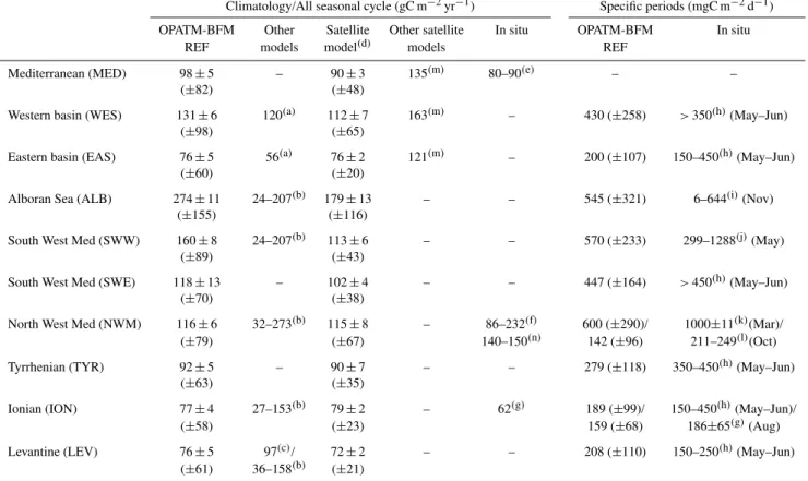
Table 1.Regional averages of net primary production presented as annual value and for shorter specific period selected on the basis of data availability. Data indicate typical mean and (for climatology only) related inter-annual variability, computed as mean and standard deviations of the six annual mean values, respectively. The average of the six standard deviations is reported in parentheses as the typical intra-period variability. References:(a)Crispi et al. (2002),(b)Allen et al. (2002),(c)Napolitano et al. (2000),(d)Colella (2006),(e)Sournia (1973),
(f)Marty and Chiaverini (2002),(g)Boldrin et al. (2002),(h)Moutin and Raimbault (2002),(i)Mac´ıas et al. (2009),(j)Lohrenz et al. (2003),
(k)Moran and Estrada (2001),(l)Granata et al. (2004),(m)Bosc et al. (2004),(n)Conan et al. (1998).
Climatology/All seasonal cycle (gC m−2yr−1) Specific periods (mgC m−2d−1)
OPATM-BFM Other Satellite Other satellite In situ OPATM-BFM In situ REF models model(d) models REF
Mediterranean (MED) 98±5 – 90±3 135(m) 80–90(e) – – (±82) (±48)
Western basin (WES) 131±6 120(a) 112±7 163(m) – 430 (±258) >350(h)(May–Jun) (±98) (±65)
Eastern basin (EAS) 76±5 56(a) 76±2 121(m) – 200 (±107) 150–450(h)(May–Jun) (±60) (±20)
Alboran Sea (ALB) 274±11 24–207(b) 179±13 – – 545 (±321) 6–644(i)(Nov) (±155) (±116)
South West Med (SWW) 160±8 24–207(b) 113±6 – – 570 (±233) 299–1288(j)(May) (±89) (±43)
South West Med (SWE) 118±13 – 102±4 – – 447 (±164) >450(h)(May–Jun) (±70) (±38)
North West Med (NWM) 116±6 32–273(b) 115±8 – 86–232(f) 600 (±290)/ 1000±11(k)(Mar)/ (±79) (±67) 140–150(n) 142 (±96) 211–249(l)(Oct) Tyrrhenian (TYR) 92±5 – 90±7 – – 279 (±118) 350–450(h)(May–Jun)
(±63) (±35)
Ionian (ION) 77±4 27–153(b) 79±2 – 62(g) 189 (±99)/ 150–450(h)(May–Jun)/ (±58) (±23) 159 (±68) 186±65(g)(Aug) Levantine (LEV) 76±5 97(c)/ 72±2 – – 208 (±110) 150–250(h)(May–Jun)
(±61) 36–158(b) (±21)
0.25 mg chl-am−3. The DCM was found at roughly the same depth from the Alboran Sea area up to the western part of the Algerian region (5◦E, Fig. 4a, T1). In the south Ionian Sea
and the Levantine region, the DCM was observed to occur at a quite uniform depth of approximately 110 m with aver-age chlorophyll concentrations of approximately 0.1 mg
chl-am−3. The north-south transects, which cut across the west-ern MS, the central MS and the Levantine (T2, T3 and T4 in Fig. 1), indicate a gradient with a shallower DCM in the northern reaches of the MS, wherein chlorophyll concen-trations of approximately 0.15–0.25 mg chl-am−3were ob-served at a depth of 70 m in the western sub-basin (Fig. 4b, T2) and 0.10–0.15 mg chl-am−3were observed at a depth of 110 m in the Levantine region (Fig. 4b, T4). The DCM in the Ionian transect (T3, Fig. 4c) also follows a gradient with deeper values in the southern part.
The west-east DCM gradient that was observed by Turley et al. (2000; see their Table 2) and Moutin and Raimbault (2002; see their Table 1) in the period between May and June is another characteristic feature reproduced by the model.
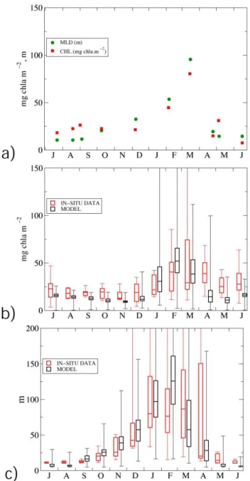
We compare (Fig. 5) the average seasonal cycle in MLD and chlorophyll standing stocks obtained with the model output in a 1◦ box around the DYFAMED station and the
Fig. 4a. Vertical section of average chlorophyll (mg chl-a m−3) along the T1 zonal transect (see Fig. 1) from OPATM-BFM REF run averaged for the period 1999–2004. Crossing lines between transect T1 and regions are indicated by dashed red lines.
Fig. 4b. Vertical section of average chlorophyll (mg chl-am−3)
from OPATM-BFM REF run along the T2 (left) and T4 (right) meridional transects (see Fig. 1) for the 6-yr period 1999–2004. Crossing lines between transect T2 and regions are indicated by dashed red lines.
model run, with peak biomass in February both in model re-sults and in situ. The inter-quartile range for March is larger in the DYFAMED site than in the model. The main discrep-ancy between data and model simulation is related to late bloom period (Fig. 5b): in April the model shows a fast de-crease in concentration, whilst the data show higher concen-trations. In the same period modeled MLD presents inter-quartile range values lower than those observed in the DY-FAMED site (Fig. 5c).
The chlorophyll seasonal cycle that was described above for the DYFAMED station is consistent with the general
Fig. 4c. Vertical section of average chlorophyll (mg chl-am−3)
from OPATM-BFM REF run along the T3 meridional transect (see Fig. 1) for the period 1999–2004. Crossing lines between transect T3 and regions are indicated by dashed red lines.
Table 2. Horizontal averages of vertically integrated net primary productions (gC m−2yr−1)for selected model simulations. Data indicate typical mean and (for climatology only) related inter-annual variability, computed as mean and standard deviations of the six annual mean values, respectively. The average of the six stan-dard deviations is reported in parentheses as the typical intra-period variability.
OPATM-BFM OPATM-BFM OPATM-BFM
REF without ATI REF (k+0.01)
Mediterranean (MED) 98±5 95±4 87±7
(±82) (±85) (±74)
Western basin (WES) 131±6 127±5 120±7
(±98) (±103) (±89)
Eastern basin (EAS) 76±5 73±4 64±8
(±60) (±61) (±53)
Alboran Sea (ALB) 274±11 273±12 243±7
(±155) (±129) (±137)
South West Med (SWW) 160±8 156±7 145±6
(±89) (±91) (±79)
South West Med (SWE) 118±13 113±12 109±12
(±70) (±71) (±66)
North West Med (NWM) 116±6 111±6 108±7
(±79) (±84) (±75)
Tyrrhenian (TYR) 92±5 88±5 88±6
(±63) (±66) (±62)
Ionian (ION) 77±4 74±3 68±6
(±58) (±61) (±54)
Levantine (LEV) 76±5 73±6 60±11
Fig. 5. (a)Seasonal cycle of integrated chlorophyll and mixed layer depth at DYFAMED station for the year 1998; (b) climatologi-cal seasonal cycle of integrated chlorophyll from in situ data and model results aggregated as monthly medians; (c)climatological seasonal cycle of mixed layer depth from in situ data and model results aggregated as monthly medians. In situ climatology data is derived from DYFAMED dataset for the period 1991–1999 (Marty and Chavi`erini, 2002). Model outputs are monthly medians for the period 1999–2004 considering a 1 degree box centered on DY-FAMED station position. Boxes values represent, from lower to higher values, minimum, 25th percentile, median, 75th percentile and maximum.
behaviour of the chlorophyll that was modelled in the NWM area in the model. This offers support to the hypothesis of Marty and Chiav´erini (2002), who argued that
the chlorophyll seasonal cycle that has been observed at the DYFAMED station is representative of a larger area in which open ocean processes drive the biotic dynamics of the ecosystem.
At the basin scale, the temporal and spatial variability of surface chlorophyll concentrations simulated by the model are compared to satellite results (Fig. 6). Regionally ag-gregated median values of modelled surface chlorophyll are compared to SeaWiFS level 4 composites that were repro-cessed using a regional algorithm (Volpe et al., 2007) and interpolated onto the model grid. We applied the algorithm described in Vichi et al. (2007b) to compare model chloro-phyll with surface observation.
A clear seasonal cycle is present in all of the regions with maximum values during February or March and min-imum values in summer. This is also the period when the largest relative underestimation of the model is observed when compared to satellite data, which was typically lower than 0.05 mg chl-am−3. In the NWM region in particu-lar, the simulated spring bloom terminates one month ear-lier than observations. Such model behaviour may be related to the MLD dynamics shown in Fig. 5 for DYFAMED sta-tion, which is representative of the NWM region. Spatial differences in the range between 25th and 75th percentiles around the median value appear to be quite similar between the model and satellite data, as already observed in Lazzari et al. (2010) with the analyses done for the operational model.
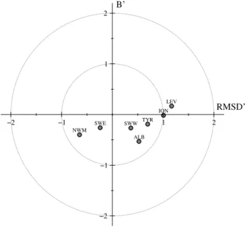
The model skill in each region can be graphically sum-marised with a target diagram (Jolliff et al., 2009). This di-agram (Fig. 7) reports on thex-axis the unbiased root mean square difference (RMSD’) between model results and ref-erence data, whereas they-axis indicates the bias (B’) with respect to the reference data (in this case satellite). Both axes are normalised based on the variance of the satellite data. We computed B’ and RMSD’ for the climatological seasonal cycle of each grid cell of the model with respect to the ref-erence satellite grid cell (interpolated onto the model grid), and we collapsed each cloud of data by computing median values of B’ and RMSD’ for each region. Because RMSD’ is intrinsically positive, the sign of thex-axis was used to indicate whether the model variance was higher (x >0) or lower (x <0) than the satellite variance. The model results and reference data perfectly agree for points that are plotted at the centre of the target. All of the western regions are in-side of the unitary circle, which indicates a good agreement with observations. The eastern regions are outside of the uni-tary circle; however, in those areas, the absolute differences between model and data are very low due to the marked olig-otrophic regime.
! !"# !"$ !"% !"&
'()*+,-)'
!
. /01
! !"# !"$ !"% !"&
'()*+,-)'
!
. 234
! !"# !"$ !"% !"&
'()*+,-)'
!
. 533
! !"# !"$ !"% !"&
'()*+,-)'
!
. 536
! !"# !"$ !"% !"&
'()*+,-)'
!
. 789
! !"!: !"; !";: !"#
'()*+,-)'
!
. <=2
>?0 /?@ 56A =B7 2=C D6B >/2 E61 4/9 /A9 4/8 >?2
! !"!: !"; !";: !"#
'()*+,-)'
!
. 06C
Fig. 6. Surface chlorophyll seasonal cycle (mg chl-am−3) for the period 1999–2004 simulated by OPATM-BFM model (solid red lines = median, dashed red lines = 25 and 75 percentile) compared with data from SeaWIFs (box-plot). Data are spatially aggregated (spatial median) in regions corresponding to those presented in Fig. 1.
3.2 Net primary production
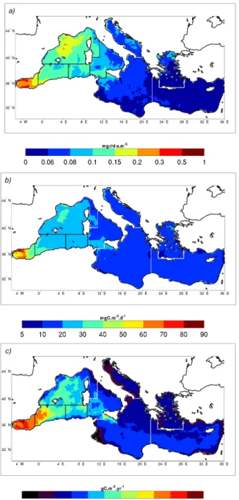
Climatological maps (1999–2004 period) of model-derived NPP and chlorophyll distribution (Fig. 8) show that surface chlorophyll, surface net primary production and vertically integrated NPP (int-NPP hereafter) differ, even though all these quantities show a west-east gradient.
The most productive pelagic areas, with respect to surface NPP, include the Alboran Sea and the NWM region, whereas the eastern Mediterranean (including the ION and LEV re-gions) is remarkably uniform.
The Alboran Sea production is correlated with the circula-tion patterns present in the area (see Supplement, part 1): ver-tical velocities enrich the surface Atlantic waters with nutri-ents that are subsequently advected horizontally through the gyres present in the area. The principal sites of vertical flux are located in the Gibraltar Strait and along the northern coast of the Alboran Sea. The north-south gradient of int-NPP in
ALB SWW SWE NWM
TYR ION
LEV
!2 !1 1 2
RMSD’
!2
!1 1 2
B’
Fig. 7.Target diagram comparing model-derived seasonal cycle in surface chlorophyll concentrations with those derived from SeaW-IFs for the different regions defined in Fig. 1. Each dot is the median of the temporal skill of each pixel for the specific regions described in Fig. 1.
the western basin is less evident than that for surface NPP, moreover a south-north int-NPP gradient can be observed in the Levantine region. A relative maximum of int-NPP rates appears along the south-western Sicilian coast, which can be ascribed to the persistent wind-driven upwelling events that are observed in this area (B´eranger et al., 2004). The effects of riverine input on int-NPP values are very weak.
Table 1 shows annual int-NPP for several regions (simu-lated period 1999–2004) from model experiments and satel-lite estimates as well as in situ data.
Fig. 8.Model-derived climatology of(a)annual surface chlorophyll concentration (mg chl-am−3);(b)surface net primary production (mgC m−3d−1); (c) vertically integrated net primary production (gC m−2yr−1).
measured values in excess of 350 mgC m−2d−1 in the western area and 150 to 450 mgC m−2d−1 in the east-ern basin (May–June 1996, Minos Cruise). OPATM-BFM estimates for the same period of the year are 430±258 mgC m−2d−1 and 200±107 mgC m−2d−1, re-spectively. The seasonal variability (OPATM-BFM REF
column, number in parentheses) is higher in the model than satellite-based estimates.
In the Alboran Sea, which is known to be the most pro-ductive MS area (Siokou-Frangou et al., 2010), our model estimates a production rate of 274±11 gC m−2yr−1. Field observations do not cover all seasons; however, a compar-ison can be made for November 2003, when Mac´ıas et al. (2009) reported primary production data characterised by high spatial variability (6–644 mgC m−2d−1) while our cur-rent model estimate is 545±321 mgC m−2d−1.
The elevated production signal from the Alboran Sea prop-agates into the Algerian region, which generates a spatial gradient that marks the declining influence of the Gibraltar Strait dynamics. The simulated annual budgets for the SWW and SWE areas are 160±8 and 118±13 gC m−2yr−1, re-spectively. An analysis by Lohrenz et al. (1988) of the Al-gerian Current (western part) in May period reported values ranging from 299 to 1288 mgC m−2d−1, whereas the model average results for the SWW are 570±233 mgC m−2d−1 for May. Moutin and Raimbault (2002) reported an int-NPP rate for the SWE area that was in excess of 450 mgC m−2d−1, whereas the model results for the same period are 447±164 mgC m−2d−1.
The difference in int-NPP between the NWM (116 gC m−2yr−1) and SWE (118 gC m−2yr−1) regions is very small, in contrast to surface properties in these regions. Experimental data also do not show a clear gradient in terms of int-NPP (Moutin and Raimbault, 2002; see their Fig. 1). Conan et al. (1998) estimated an int-NPP in the range of 140–150 gC m−2yr−1for the years of 1992–1993 (NWM region), whereas other 14C measurements for the Catalan-Balearic region range from 1000±1 mgC m−2d−1 (March period, Moran and Estrada, 2001) to 211–249 mgC m−2d−1 (October period, Granata et al., 2004). The DYFAMED station measurements presented highly variable int-NPP rates, ranging from 86 to 232 gC m−2yr−1 for the 1993– 1999 period, with an average of 156 gC m−2yr−1 (Marty and Chiav´erini, 2002). A high degree of seasonal variability was also obtained in a one-dimensional modelling study for the same area and in other sites across the MS (Allen et al., 2002).
Fig. 9. Temporal series of integrated net primary production (gC m−2yr−1)averaged for the 7 areas of Fig. 1 (black line); cli-matological values for the period 1999–2004 (brown shading), and annual averages (red lines).
of 159±68 mgC m−2d−1 are in fair agreement with the measured rates of 186±65 mgC m−2d−1 (Boldrin et al., 2002). Similar agreement holds for the Levantine region.
The temporal series of int-NPP values from the standard run is shown in Fig. 9. All the regions are characterised by a strong seasonal cycle. As shown in Table 1, the inter-annual variability in annual int-NPP (red lines in Fig. 9) is lower than that of the seasonal cycle (black lines in Fig. 9). In the ALB region, the maxima are spread across the period from January–June. The western and eastern regions differ primarily in the declining phase of int-NPP: in the western regions, the int-NPP winter peak is sustained for a longer period than in the eastern reaches.
Because the light extinction factor adopted in these cal-culations is characterised by substantial uncertainty, we per-formed a simulation to evaluate the impact of increasing the extinction factor (k)by 0.01 m−1 (around 30 % of min-imum value). This analysis demonstrates the sensitivity of the system to k and results in a reduction in int-NPP of
approximately 10 gC m−2yr−1. Further, the sensitivity of model output tokis largely confined to surface fields. This test revealed that the belt-like pattern of higher int-NPP, which is evident in the south Ionian and south Levantine regions as depicted in Fig. 8, is sensitive tok because the higher int-NPP rates that are present in the eastern area dis-appear with a 30 % increase ink(image not shown).
A comparison between different simulations (Table 2), performed with varying ATIs, indicates that the impact of these sources on the annual int-NPP budget amounts to an increase of 3 gC m−2yr−1 and varies across different sub-basins over a range of 3–5 gC m−2yr−1.
4 Discussion
Numerical simulations give a virtual representation of reality which can be sampled at high frequency in both space and time and, therefore, allow us to fully cover and quantify the spatial and temporal variability of the biogeochemical and physical characteristics of pelagic systems and within each of its regions.
According to our basin-scale simulation, the normalised, tiaveraged inter-quartile range (IQR) around the me-dian chlorophyll concentration was between 60 % (ALB) and 35 % (SWE) and typically of the order of 45 %, whereas the normalised IQR was between 60 % (ALB) and 45 % (SWE) and typically of the order of 52 % for the int-NPP. These ranges imply that single measurements can rarely provide ac-curate representations of regional biogeochemical conditions or annual productivity budgets.
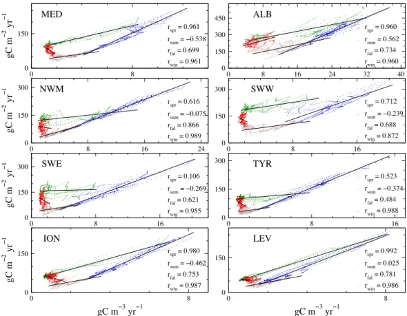
Similarly, for all the investigated regions, the instanta-neous spatial variability of the int-NPP can exceed a nor-malised IQR of 100 % at any given moment, which high-lights the need of an appropriate spatial sampling frequency. Satellite-derived information may provide important knowledge about sea surface biogeochemical characteristics; however, our simulations indicate that the correlation be-tween surface productivity and integrated NPP throughout the MS is seasonally variable (Fig. 10). In general, the cor-relation is higher during winter period (January–February– March) and lower during summer period (July–August– September). This suggests a decoupling of surface and sub-surface dynamics due to stratification in summer. It is worth noting that during spring and winter, the relationship between int-NPP and surface productivity in the MS followed a linear relationship (r=0.961). Conversely, during summer the cor-relation between int-NPP and surface productivity was nega-tive with lower correlation coefficient (r= −0.538).
0 8 0
150
gC m
!
2 yr
!
1
r
spr = 0.961
r
sum = !0.538
r
fal = 0.699
rwin = 0.961
0 8 16 24 32 40
0 150 300 450
r
spr = 0.960
r
sum = 0.562
r
fal = 0.734
rwin = 0.960
0 8 16 24
0 150 300
gC m
!
2 yr
!
1
rspr = 0.616
rsum = !0.075 rfal = 0.866
rwin = 0.989
0 8 16
0 150 300
rspr = 0.712
r
sum = !0.239
rfal = 0.688
rwin = 0.872
0 8 16
0 150 300
gC m
!
2 yr
!
1
rspr = 0.106
r
sum = !0.269
rfal = 0.621
rwin = 0.955
0 8 16
0 150 300
rspr = 0.523
rsum = !0.374 r
fal = 0.484
r
win = 0.988
0 8
gC m!3 yr!1 0
150
gC m
!
2 yr
!
1
rspr = 0.980
rsum = !0.462 rfal = 0.753
rwin = 0.987
0 8
gC m!3 yr!1 0
150
rspr = 0.992
rsum = 0.025
rfal = 0.781
rwin = 0.986 MED
NWM
SWE
ION
ALB
SWW
TYR
LEV
Fig. 10. Scatter plots of integrated (gC m−2yr−1) versus surface (gC m−3yr−1) net primary production: each point represents the 10-day regional average in the period 1999–2004 for the MS and the 7 areas defined in Fig. 1. Points are colored according to seasons: winter (blue, January–February–March), spring (green, April–May–June), summer (red, July–August–September) and fall (brown, October–November– December). Black lines represent the linear regressions, whose correlation coefficientsrare also shown.
when considering environmental regulations. Specifi-cally, adopting the Nixon classification of trophic regimes (Nixon, 1995), our estimates indicate that, on average, the MS is oligotrophic (int-NPP<100 gC m−2yr−1), how-ever, the western MS, particularly the Alboran Sea area, is mesotrophic (int-NPP between 100 and 300 gC m−2yr−1), while the eastern region is typically oligotrophic.
In contrast to common perceptions, the SWW region appears to be more productive than the NWM region.
Among the bio-provinces introduced by Longhurst (1995) for the Global Ocean we found that the Longhurst model 3 (Lm 3 “subtropical nutrient-limited winter-spring produc-tion period”) was the closest to the results of the simulations presented; Lm 3 was indeed associated by Longhurst to the MS. However, this does not imply an homogeneous situa-tion for MS. In fact Longhurst classes are qualitative, and each one encompasses a spectrum of quantitative trends as illustrated by the Longhurst diagrams for each region in the MS, as well as the deep convection area (grid point located in NWM at 5.0625◦E–42.1258◦N), given in Fig. 11. From the analysis of the Longhurst diagrams the west-east gradient in chlorophyll accumulation (Fig. 11) is evident. The same
a) JUL AUG SEP OCT NOVDEC JAN FEB MAR APR MAY JUN 0 0.1 0.2 0.3 0.4 0.5 chl− a
(mg chla m
−3)
JUL AUG SEP OCT NOVDEC JAN FEB MAR APR MAY JUN 0 300 600 900 1200
NPP, GRZ (mg C m
−2 d −1) Alboran Sea
JUL AUG SEP OCT NOVDEC JAN FEB MAR APR MAY JUN −200 −175 −150 −125 −100 −75 −50 −25 0
MLD, PCL (m)
b) JUL AUG SEP OCT NOV DEC JAN FEB MAR APR MAY JUN
0 0.1 0.2 0.3 0.4 0.5 chl− a
(mg chla m
−3)
JUL AUG SEP OCT NOV DEC JAN FEB MAR APR MAY JUN 0 300 600 900 1200
NPP, GRZ (mg C m
−2 d −1) SWW region
JUL AUG SEP OCT NOV DEC JAN FEB MAR APR MAY JUN −200 −175 −150 −125 −100 −75 −50 −25 0
MLD, PCL (m)
c) JUL AUG SEP OCT NOV DEC JAN FEB MAR APR MAY JUN
0 0.1 0.2 0.3 0.4 0.5 chl− a
(mg chla m
−3)
JUL AUG SEP OCT NOV DEC JAN FEB MAR APR MAY JUN 0 300 600 900 1200
NPP, GRZ (mg C m
−2 d −1) SWE region
JUL AUG SEP OCT NOV DEC JAN FEB MAR APR MAY JUN −200 −175 −150 −125 −100 −75 −50 −25 0
MLD, PCL (m)
d) JUL AUG SEP OCT NOV DEC JAN FEB MAR APR MAY JUN
0 0.1 0.2 0.3 0.4 0.5 chl− a
(mg chla m
−3)
JUL AUG SEP OCT NOV DEC JAN FEB MAR APR MAY JUN 0 300 600 900 1200
NPP, GRZ (mg C m
−2 d −1) NWM region
JUL AUG SEP OCT NOV DEC JAN FEB MAR APR MAY JUN −200 −175 −150 −125 −100 −75 −50 −25 0
MLD, PCL (m)
e) JUL AUG SEP OCT NOV DEC JAN FEB MAR APR MAY JUN
0 0.1 0.2 0.3 0.4 0.5 chl− a
(mg chla m
−3)
JUL AUG SEP OCT NOV DEC JAN FEB MAR APR MAY JUN 0 300 600 900 1200
NPP, GRZ (mg C m
−2 d −1) Tyrrhenian Sea
JUL AUG SEP OCT NOV DEC JAN FEB MAR APR MAY JUN −200 −175 −150 −125 −100 −75 −50 −25 0
MLD, PCL (m)
f) JUL AUG SEP OCT NOV DEC JAN FEB MAR APR MAY JUN
0 0.1 0.2 0.3 0.4 0.5 chl− a
(mg chla m
−3)
JUL AUG SEP OCT NOV DEC JAN FEB MAR APR MAY JUN 0 300 600 900 1200
NPP, GRZ (mg C m
−2 d −1) Ionian Sea
JUL AUG SEP OCT NOV DEC JAN FEB MAR APR MAY JUN −200 −175 −150 −125 −100 −75 −50 −25 0
MLD, PCL (m)
g) JUL AUG SEP OCT NOVDEC JAN FEB MAR APR MAY JUN
0 0.1 0.2 0.3 0.4 0.5 chl− a
(mg chla m
−3)
JUL AUG SEP OCT NOVDEC JAN FEB MAR APR MAY JUN 0 300 600 900 1200
NPP, GRZ (mg C m
−2 d
−1
)
Levantine Sea
JUL AUG SEP OCT NOVDEC JAN FEB MAR APR MAY JUN −300 −275 −250 −225 −200 −175 −150 −125 −100 −75 −50 −25 0
MLD, PCL (m)
h) JUL AUG SEP OCT NOV DEC JAN FEB MAR APR MAY JUN
0 0.2 0.4 0.6 0.8 chl− a
(mg chla m
−3)
JUL AUG SEP OCT NOV DEC JAN FEB MAR APR MAY JUN 0 300 600 900 1200 1500 1800
NPP, GRZ (mg C m
−2 d
−1
)
Deep convection (5.0625 o E − 42.1258 o N)
JUL AUG SEP OCT NOV DEC JAN FEB MAR APR MAY JUN −1500 −1250 −1000 −750 −500 −250 0
MLD, PCL (m)
The seasonal variability (number in parentheses, Table 1) is higher in the model results than in the satellite data. Such variability, however, is consistent with observations at the DYFAMED site (Marty and Chiav´erini, 2002) and time se-ries measurements by Psarra et al. (2000) in the eastern MS. The temporal variability of int-NPP also qualitatively agrees with variability in short wave radiation and wind speed (im-ages not shown); in fact, for both forcings, the seasonal cycle is the strongest component of the signal, whereas the vari-ability of the annual average is very low. The same argu-ments are valid for the variability of the MLD.
The sensitivity analysis performed indicates that uncer-tainty ink is associated with a 10 % uncertainty in the es-timation of int-NPP. This suggests that even if the present model configuration can be considered an useful tool to esti-mate the spatial-temporal variability of the variables consid-ered, an increase in our quantitative knowledge of the factors regulating the system is required for more accurate estimates. The impact of ATIs are low in terms of large-scale averaged int-NPP but could be relevant when considering new produc-tion.
5 Conclusions
A model based synthesis of the chlorophyll concentrations and net primary production rates in the Mediterranean Sea for the 1999–2004 period is presented in this study. Model simulations illustrate the high spatial and temporal variability of chlorophyll concentrations and integrated NPP, and high-light the importance of considering these variables when per-forming basin-wide budgets and exploring basin-wide tem-poral variability.
According to the results obtained, the following summary points can be concluded:
– The model outcomes agree fairly well with prior in situ observations.
– The seasonal cycle signal of the integrated NPP domi-nates over the inter-annual variability when large scale averages are considered.
– The horizontal averages over selected regions show a clear spatial gradient in NPP and chlorophyll standing stocks from west to east.
– The north-south patterns are different with respect to surface and integrated properties.
– On average the model results are in line with the Longhurst biological domain “subtropical nutrient-limited winter-spring production period”.
– Depth of nutricline and grazing rates are important pa-rameters to explain spatial differences between MS re-gions which are not resolved using the Longhurst clas-sification scheme (Longhurst, 1995).
– The impact of atmospheric and terrestrial inputs on the annual budget of the integrated NPP (new production) is in the range of 3–5 gC m−2yr−1.
– Moreover, the impact of a 30 % increase in the extinc-tion factor (k) on the integrated NPP annual budget is approximately 10 gC m−2yr−1.
The spatial and temporal variability of simulated chlorophyll and int-NPP ranges suggests that a 3-D model approach con-stitutes an important tool for exploring seasonal and spatial variability in land-remote oceanic areas, in particular within the context of establishing conservation policies.
Appendix A
Transport equations formulation
The ocean 3-D fields from the MED16 model at 1/16◦ reso-lution are horizontally interpolated on a 1/8◦resolution grid while the original vertical grid is maintained. In more details, the working meshgrid is based on 1/8◦ longitudinal scale factors (e1)and on 1/8◦cos(ϕ)latitudinal scale factor (e2). The vertical meshgrid (e3)accounts for 43 vertical z-levels: 13 in the first 200 m depth, 18 between 200 and 2000 m, 12 below 2000 m.
The temporal scheme is explicit forward time scheme for the advection term (A) whereas an implicit time step is adopted for the vertical diffusion (Dv).
In numerical terms, the transport reaction equations are:
A =
"
1
e1e2e3
1 e2e3ctiu
1i +
1 e1e3ctiv
1j +
1 e1e2ctiw
1k
!#
(A1) The advection term Acorresponds to the budget of all the fluxes across the boundaries of the cell with index (i lon-gitude, j latitude,k depth) normalized on the cell volume (e1e2e3).
Dv=
1
e3
1 1k
kv
e3
1cti+1
1k
(A2)
wherekvis the vertical eddy diffusivity coefficient andciare the concentration at timet+1.
The vertical diffusion term (Dv) is calculated by an im-plicit forward time scheme to increase the stability, espe-cially in the vertical mixing phase where vertical diffusion coefficient can be very high.
The sinking termSis a vertical flux:
S=
"
1
e1e2e3
1 e1e2ctiws
1k
!#
(A3)
Appendix B
Photosynthesis formulation
The carbon (C) fixation, Eq. (B1) and chlorophyll (chl) syn-thesis, Eq. (B2), read:
∂C
∂t =gpp−rsp−exu−predC (B1)
∂chl
∂t =f n,p
P ρchl(gpp−rsp−exu)−tratechl+chlREL−predchl (B2)
in particular the gross productivity rate is defined as
gpp=pCmfEfTfSC (B3)
wherePmCis the maximum potential uptake,fT,fSare the limitations for temperature and silicates (diatoms only),fE, Eq. (B3), is the limiting factor for photosynthetic available radiationI (z).
fE= 1−e−
αchl(P )I (z)θ PmC
!
(B4)
trate=max(psdchl(P )(1−f n,p
P ),0) (B5)
ChlREL=min(0,gpp−rsp)max(Chl−pqchlc(P )C,0) (B6) ρchlis the rate of chlorophyll synthesis for unit of carbon fix-ation that regulates the degree of adaptfix-ation, expressed by the quota of chlorophyll over carbonθ, to the different light regimes. trate is the turnover rate based on nutrient stress andChlRELis a relaxation term toward optimal chlorophyll to carbon ratio (pqchlc(P )). fn andfp are linear limitation terms, bounded betweenpoand 1, based on nutrient to Car-bon quota.
fn→fn,p=min(fn,fp) (B7)
fn=Lpo,1
Q
NC(P )−pqnlc
pqnRc(P )−pqnlc
, (B8)
fp=Lpo,1
Q
PC(P )−pqplc(P )
pqpRc(P )−pqplc(P )
We switched fromfntofn,pin order to represent phospho-rus limitation. A full detailed description of all the biogeo-chemical model equations and correspondent parameters are included in the Supplement (part 2).
Supplementary material related to this article is available online at:
http://www.biogeosciences.net/9/217/2012/
bg-9-217-2012-supplement.zip.
Acknowledgements. This work was partially funded by projects V.E.C.T.O.R. (VulnErabilit`a delle Coste e degli ecosistemi marini italiani ai cambiamenti climaTici e loro ruolO nel ciclo del caRbonio mediterraneo; financed by Italian Special Research Fund FISR 2001), EC-FP6 SESAME-IP and Accordo di esecuzione tra CMCC ed OGS.
The simulations were carried out at the CINECA supercomputer centre (Bologna, Italy).
This work was granted access to the HPC resources of IDRIS of CNRS under allocation 2008 (i2008010227) made by GENCI. Atmospheric forcing was provided by ECMWF.
Karine B´eranger thanks the Mercator project for support to the MED16 work.
The authors thank Laurent Coppola for providing access to DYFAMED data, and Gianpiero Cossarini for fruitful discussions. Authors thank Maurizio Ribera d’Alcal`a and the other anonymous reviewer for their useful comments.
Edited by: C. Klaas
References
Allen, J. I., Somerfield, P. J., and Siddorn, J.: Primary and bacte-rial production in the Mediterranean Sea: a modelling study, J. Marine Syst., 33/34, 473–495, 2002.
Arhonditsis, G. B. and Brett, M. T.: Evaluation of the current state of mechanistic aquatic biogeochemical modelling, Mar. Ecol.-Prog. Ser., 271, 13–26, 2004.
Azov, I.: The Mediterranean Sea, a marine desert?, Mar. Pollut. Bull., 23, 225–232, 1991.
Barale, V., Jaquet, J.-M., and Ndiaye, M.: Algal blooming patterns and anomalies in the Mediterranean Sea as derived form Sea-WiFS dataset (1998–2003), Remote Sens. Environ., 112, 3300– 3313, 2008.
Barnier, B.: Forcing the Ocean, in: Ocean Modeling and Param-eterization, edited by: Chassignet, E. P. and Verron, J., NATO Sciences Series, Serie C: Mathematical and Physical Sciences, vol. 516., 45–80, Kluwer Academic Publishers. Printed in the Netherlands, 1998.
Behrenfeld, M. J.: Abandoning Sverdrup’s Critical Depth Hypoth-esis on phytoplankton blooms: Ecology, 91, 977–989, 2010. B´eranger, K., Mortier, L., Gasparini, G.-P., Gervasio, L., Astraldi,
M., and Cr´epon, M.: The dynamics of the Sicily Strait: A com-prehensive study from observations and models, Deep Sea Res. Pt. II, 51, 411–440, 2004.
B´eranger, K., Mortier, L., and Cr´epon, M.: Seasonal variability of water transport through the Straits of Gibraltar, Sicily and Cor-sica, derived from a high-resolution model of the Mediterranean circulation, Prog. Oceanogr., 66, 341–364, 2005.
B´eranger, K., Testor, P., and Cr´epon, M.: Modelling water mass for-mation in the Gulf of Lion (Mediterranean Sea), WORKSHOP CIESM Monograph n◦38 on Dynamics of Mediterranean deep waters, F. Briand Eds., Monaco, 2009.
in the Mediterranean Sea, J. Geophys. Res., 115, C12041, doi:10.1029/2009JC005648, 2010.
Bergametti, G., Remoudaki, E., Losno, R., Steiner, E., and Chatenet, B.: Source, transport and deposition of atmospheric Phosphorus over the northwestern Mediterranean, J. Atmos. Chem., 14, 501–513, 1992.
B´ethoux, J. P., Morin, P., Chaumery, C., Connan, O., Gentili, B., and Ruiz-Pino, D.: Nutrients in the Mediterranean Sea, mass balance and statistical analysis of concentrations with respect to environ-mental change, Mar. Chem., 63, 155–169, 1998.
Bianchi, C. N. and Morri, C.: Marine Biodiversity of the Mediter-ranean Sea: Situation, Problems and Prospects for Future Re-search, Mar. Pollut. Bull., 40, 367–376, 2000.
Blanke, B. and Delecluse, P.: Variability of the tropical Atlantic ocean simulated by a general circulation model with two dif-ferent mixed layer physics, J. Phys. Oceanogr., 23, 1363–1388, 1993.
Boldrin, A., Miserocchi, S., Rabitti, S., Turchetto, M. M., Balboni, V., and Socal, G.: Particulate matter in the southern Adriatic and Ionian Sea: characterization and downward fluxes, J. Ma-rine Syst., 33/34, 389–410, 2002.
Bosc, E., Bricaud, A., and Antoine, D.: Seasonal and inter-annual variability in algal biomass and primary production in the Mediterranean Sea, as derived from 4 years of Sea-WiFS observations, Global Biogeochem. Cy., 18, GB1005, doi:10.1029/2003GB002034, 2004.
Brankart, J.-M. and Brasseur, P.: The general circulation in the Mediterranean Sea: a climatological approach, J. Mar. Syst., 18, 41–70, 1998.
Caddy, J. F., Refk, R., and Do-Chi, T.: Productivity estimates for the Mediterranean: evidence of accelerating ecological change, Ocean Coastal Manage., 26, 1–18, 1995.
Colella, S.: La produzione primaria nel Mar Mediterraneo da satel-lite: sviluppo di un modello regionale e sua applicazione ai dati SeaWiFS, MODIS e MERIS, Phd Thesis, Universit`a Federico II Napoli, 162 pp., 2006.
Coll, M., Piroddi, C., Steenbeek, J., Kaschner, K., Ben Rais Lasram, F., Aguzzi, J., Ballesteros, E., Bianchi, C. N., Corbera, J., Dailia-nis, T., Danovaro, R., Estrada, M., Froglia, C., Galil, B. S., Gasol, J. M., Gertwagen, R., Gil, J., Guilhaumon, F., Kesner-Reyes, K., Kitsos, M.-S., Koukouras, A., Lampadariou, N., Laxamana, E., L´opez- F´e de la Cuadra, C. M., Lotze, H. K., Martin, D., Mouil-lot, D., Oro, D., Raicevich, S., Rius-Barile, J., Saiz- Salinas, J. I., San Vicente, C., Somot, S., Templado, J., Turon, X., Vafidis, D., Villanueva, R., and Voultsiadou, E.: The Biodiversity of the Mediterranean Sea: Estimates, Patterns, and Threats, PLoS One, 5, 1–34, 2010.
Conan, P., Pujo-Pay, M., Raimbault, M., and Leveau, M.: Hydro-logical and bioHydro-logical variability of the Gulf of Lions. II Pro-ductivity on the inner edge of the North Mediterranean Current, Oceanol. Acta, 21, 767–782, 1998.
Cornell, S., Rendell, A., and Jickells, T.: Atmospheric inputs of dissolved organic Nitrogen to the oceans, Nature, 376, 243–246, 1995.
Crise, A., Allen, J. I., Baretta, J., Crispi, G., Mosetti, R., and Solidoro, C.: The Mediterranean pelagic ecosystem response to physical forcing, Prog. Oceanogr., 44, 219–243, 1999.
Crise, A., Solidoro, C., and Tomini, I.: Preparation of initial con-ditions for the coupled model OGCM and initial parameters
set-ting, MFSTEP report WP11, subtask 11310, 2003.
Crispi. G., Crise, A., and Mauri, E.: A seasonal three-dimensional study of the nitrogen cycle in the Mediterranean Sea: Part II. Verification of the energy constrained trophic model, J. Marine Syst., 20, 357–379, 1999.
Crispi, G., Mosetti, R., Solidoro, C., and Crise, A.: Nutrient cycling in Mediterranean basins: the role of the biological pump in the trophic regime, Ecol. Model., 138, 101–114, 2001.
Crispi, G., Crise, A., and Solidoro, C.: Coupled Mediterranean eco-model of the Phosphorus and Nitrogen cycles, J. Marine Syst., 33/34, 497–521, 2002.
D’Ortenzio, F. and Ribera d’Alcal`a, M.: On the trophic regimes of the Mediterranean Sea: a satellite analysis, Biogeosciences, 6, 139–148, doi:10.5194/bg-6-139-2009, 2009.
D’Ortenzio, F., Iudicone, D., de Boyer Montegut, C., Testor, P., Antoine, D., Marullo, S., Santoleri, R., and Madec G.: Seasonal variability of the mixed layer depth in the Mediterranean Sea as derived from in situ profiles, Geophys. Res. Lett., 32, L12605, doi:10.1029/2005GL022463, 2005.
Flynn, K. J.: A mechanistic model for describing dynamic multi-nutrient, light, temperature interactions in phytoplankton, J. Plankton Res., 23, 977–997, 2001.
Follows, M. J., Dutkiewicz, S., Grant, S., and Chisholm, S. W.: Emergent Biogeography of Microbial Communities in a Model Ocean, Science, 315, 1843–1846, 2007.
Foujols, M.-A., L´evy, M., Aumont, O., Madec, G.: OPA 8.1 Tracer Model Reference Manual, Institut Pierre Simon Laplace, 39 pp., 2000.
Geider, R. J., MacIntyre, H. L., and Kana, T. M.: Dynamic model of phytoplankton growth and acclimation: responses of the bal-anced growth rate and the chlorophyll a: Carbon ratio to light, nutrient-limitation and temperature, Mar. Ecol.-Prog. Ser., 148, 187–200, 1997.
Granata, T. C., Estrada, M., Zika, U., and Merry, C.: Evidence for enhanced primary production resulting from relative vorticity in-duced upwelling in the Catalan Current, Sci. Mar., 68, 113–119, 2004.
Guerzoni, S., Chester, R., Dulac, F., Herut, B., Lo¨ye-Pilot, M.-D., Measures, C., Migon, C., Molinaroli, E., Moulin, C., Rossini, P., Saydam, C., Soudine, A., and Ziveri, P.: The role of atmo-spheric deposition in the biogeochemistry of the Mediterranean Sea. Prog. Oceanogr., 44, 147–190, 1999.
Herut, B. and Krom, M.: Atmospheric input of nutrients and dust to the SE Mediterranean, in: The Impact of Desert Dust Across the Mediterranean, edited by: Guerzoni, S. and Chester, R., Kluwer Acad., Norwell, Mass., 349–358, 1996.
Jolliff, J. K., Kindle, J. C., Shulman, I., Penta, B., Friedrichs, M. A. M., Helber, R., and Arnone, R. A.: Summary diagrams for cou-pled hydrodynamic-ecosystem model skill assessment, J. Marine Syst., 76, 64–82, 2009.
Krom, M. D., Kress, N., Brenner, S., and Gordon, L. I.: Phospho-rus limitation of primary production in the eastern Mediterranean Sea, Limnol. Oceanogr., 36, 424–432, 1991.
Lazzari, P., Teruzzi, A., Salon, S., Campagna, S., Calonaci, C., Colella, S., Tonani, M., and Crise, A.: Pre-operational short-term forecasts for the Mediterranean Sea biogeochemistry, Ocean Sci., 6, 25–39, 2010,
http://www.ocean-sci.net/6/25/2010/.
Sutherland, S. C.: Impact of climate change and variability on the global oceanic sink of CO2, Global Biogeochem. Cy., 24, GB4007, doi:10.1029/2009GB003599, 2010.
L¨oye-Pilot, M. D., Martin, J. M., and Morelli, J.: Atmospheric input of inorganic Nitrogen to the western Mediterranean, Bio-geochem., 9, 117–134, 1990.
Lohrenz, S. E., Wiesenburg, D. A., DePalma, I. P., Johnson K. S., and Gustafson D. E.: Inter-relationship among primary produc-tion, chlorophyll, and environmental conditions in frontal regions of the western Mediterranean Sea, Deep-Sea Res., 35, 793–810, 1988.
Longhurst, A. R.: Seasonal cycles of pelagic production and con-sumption, Prog. Oceanogr., 36, 77–167, 1995.
Ludwig, W., Dumont, E., Meybeck, M., and Heussner, S.: River discharges of water and nutrients to the Mediterranean and Black Sea: Major drivers for ecosystem changes during past and future decades?, Progr. Oceanogr., 80, 199–217, 2009.
Mac´ıas, D., Navarro, G., Bartual, A., Echevarr´ıa, F., and Huertas, I. E.: Primary production in the Strait of Gibraltar: Carbon fixation rates in relation to hydrodynamic and phytoplankton dynamics, Estuar. Coast. Shelf S., 83, 115–264, 2009.
Madec, G., Delecluse, P., Imbard, M., and L´evy, C.: OPA, release 8, Ocean General Circulation reference manual, Technical report 96/xx, LODYC/IPSL, France, February, 1997.
Mann, K. H. and Lazier, J. R. N.: Dynamics of Marine Ecosystems, Blackwell Publishing, 496 pp., 2006.
Marty, J. C. and Chiav´erini, J.: Seasonal and interannual variations in phytoplankton production at the DYFAMED time -series sta-tion (1991–1999), Deep-Sea Res. Pt. II, 49, 2017–2030, 2002. Mor´an, X. A. G. and Estrada, M.: Short term variability of
photo-synthetic parameters and particulate and dissolved primary pro-duction in the Alboran Sea (SW Mediterranean), Mar. Ecol.-Prog. Ser., 212, 53–67, 2001.
Morel, A. and Gentili, B.: The dissolved yellow substance and the shades of blue in the Mediterranean Sea, Biogeosciences, 6, 2625–2636, doi:10.5194/bg-6-2625-2009, 2009.
Moutin, T. and Raimbault, P.: Primary production, Carbon export and nutrients availability in western and eastern Mediterranean Sea in early summer 1996 (MINOS cruise), J. Marine Syst., 33/34, 273–288, 2002.
Napolitano, E., Oguz, T., Malanotte-Rizzoli, P., Yilmaz, A., and Sansone, E.: Simulations of biological production in the Rhodes and Ionian basins of the eastern Mediterranean, J. Marine Syst., 24, 277–298, 2000.
Nixon, S. W.: Coastal marine eutrophication: a definition, social causes, and future concerns, Ophelia, 41, 199–219, 1995. Pinardi, N. and Masetti, E.: Variability of the large scale general
circulation of the Mediterranean Sea observations and modelling: a review, Palaeogeogr. Palaeocl., 158, 153–173, 2000.
Psarra, S., Tselepides, A., and Ignatiades, L.: Primary production in the oligotrophic Cretan Sea (NE Mediterranean): seasonal and interannual variability, Prog. Oceanogr., 46, 187–204, 2000. Pugnetti, A., Camatti, E., Mangoni, O., Morabito, G., Oggioni, A.,
and Saggiomo, V.: Phytoplankton production in italian fresh-water and marine ecosystems: state of the art and perspectives, Chem. Ecol., 22, S49–S69, 2006.
Reynaud, T., LeGrand, P., Mercier, H., and Barnier, B.: A new anal-ysis of hydrographic data in the Atlantic and its application to an inverse modelling study, International WOCE Newsletter, 32, 29–31, 1998.
Ribera d’Alcal`a, M., Civitarese, G., Conversano, F., and Lavezza, R.: Nutrient ratios and fluxes hint at overlooked processes in the Mediterranean Sea, J. Geophys. Res., 108, 8106, doi:10.1029/2002JC001650, 2003.
Riley, G. A.: Transparency-chlorophyll relations, Limnol. Oceanogr., 20, 150–152, 1975.
Robarts, D. R., Zohary, T., Waiser, M. J., and Yacobi, Y. Z.: Bac-terial abundance, biomass, and production in relation to phy-toplankton biomass in the Levantine Basin of the southeastern Mediterranean Sea, Mar. Ecol.-Prog. Ser., 137, 273–281, 1996. Sarmiento, J. L. and Gruber, N.: Ocean Biogeochemical Dynamics,
PUP, 526 pp., 2006.
Siokou-Frangou, I., Christaki, U., Mazzocchi, M. G., Montresor, M., Ribera d’Alcal´a, M., Vaqu´e, D., and Zingone, A.: Plank-ton in the open Mediterranean Sea: a review, Biogeosciences, 7, 1543–1586, doi:10.5194/bg-7-1543-2010, 2010.
Sournia, A.: La production primaire planctonique en M´editerrane´ee: Essai de mise `a jour. Bull. Etude Commun. M´editer., 5, 1–128, 1973.
Thingstad, T. F. and Rassoulzadegan, F.: Nutrient limitations, mi-crobial food webs, and “biological C-pumps”: suggested inter-actions in a P-limited Mediterranean, Mar. Ecol.-Prog. Ser., 117, 299–306, 1995.
Turley, C. M., Bianchi, M., Christaki, U., Conan, P., Harris, J. R. W., Psarra, S., Ruddy, G., Stutt, E. D., Tselepides, A., and Van Wambeke, F.: Relationship between primary producers and bac-teria in oligotrophic sea: the Mediterranean and biogeochemical implication, Mar. Ecol.-Prog. Ser., 193, 11–18, 2000.
Uppala, S. M., Kallberg, P. W., Simmons, A. J., Andrae, U., da Costa Bechtold, V., Fiorino, M., Gibson, J. K., Haseler, J., Her-nandez, A., Kelly, G. A., Li, X., Onogi, K., Saarinen, S., Sokka, N., Allan, R. P., Andersson, E., Arpe, K., Balmaseda, M. A., Beljaars, A. C. M., van de Berg, L., Bidlot, J., Bormann, N., Caires, S., Chevallier, F., Dethof, A., Dragosavac, M., Fisher, M., Fuentes, M., Hagemann, S., H´olm, E., Hoskins, B. J., Isak-sen, L., JansIsak-sen, P. A. E. M., Jenne, R., McNally, A. P., Mahfouf, J.-F., Morcrette, J.-J., Rayner, N. A., Saunders, R. W., Simon, P., Sterl, A., Trenberth, K. E., Untch, A., Vasiljevic, D., Viterbo, P., and Woollen, J.: The ERA-40 re-analysis, Quart. J. R. Meteorol. Soc., 131, 2961–3012, 2005.
Vichi, M., Pinardi, N., and Masina, S.: A generalized model of pelagic biogeochemistry for the global ocean ecosystem, Part I: Theory, J. Marine Syst., 64, 89–109, 2007a.
Vichi, M., Masina, S., Navarra, A.: A generalized model of pelagic biogeochemistry for the global ocean ecosystem, Part II: Numer-ical simulations, J. Marine Syst., 64, 110–134, 2007b.