Sensitivity of the simulated precipitation to changes in convective relaxation time scale

(1)

Ann. Geophys., 28, 1827–1846, 2010 www.ann-geophys.net/28/1827/2010/ doi:10.5194/angeo-28-1827-2010

Annales

Geophysicae

Sensitivity of the simulated precipitation to changes in convective

relaxation time scale

S. K. Mishra1,2and J. Srinivasan3,4

1_{National Center for Atmospheric Research, Boulder, CO, USA}

2_{Department of Computer Science, University of Colorado, Boulder, CO, USA} 3_{Divecha Centre for Climate Change, Bangalore, India}

4_{Centre for Atmospheric and Oceanic Sciences, Indian Institute of Science, Bangalore, India}

Received: 4 March 2010 – Revised: 11 August 2010 – Accepted: 26 August 2010 – Published: 6 October 2010

Abstract. The paper describes the sensitivity of the simu-lated precipitation to changes in convective relaxation time scale (TAU) of Zhang and McFarlane (ZM) cumulus param-eterization, in NCAR-Community Atmosphere Model ver-sion 3 (CAM3). In the default configuration of the model, the prescribed value of TAU, a characteristic time scale with which convective available potential energy (CAPE) is re-moved at an exponential rate by convection, is assumed to be 1 h. However, some recent observational findings sug-gest that, it is larger by around one order of magnitude. In order to explore the sensitivity of the model simulation to TAU, two model frameworks have been used, namely, aqua-planet and actual-aqua-planet configurations. Numerical integra-tions have been carried out by using different values of TAU, and its effect on simulated precipitation has been analyzed.

The aqua-planet simulations reveal that when TAU in-creases, rate of deep convective precipitation (DCP) de-creases and this leads to an accumulation of convective in-stability in the atmosphere. Consequently, the moisture con-tent in the lower- and mid- troposphere increases. On the other hand, the shallow convective precipitation (SCP) and large-scale precipitation (LSP) intensify, predominantly the SCP, and thus capping the accumulation of convective insta-bility in the atmosphere. The total precipitation (TP) remains approximately constant, but the proportion of the three com-ponents changes significantly, which in turn alters the verti-cal distribution of total precipitation production. The vertiverti-cal structure of moist heating changes from a vertically extended profile to a bottom heavy profile, with the increase of TAU. Altitude of the maximum vertical velocity shifts from upper troposphere to lower troposphere. Similar response was seen

Correspondence to:S. K. Mishra (saroj@ucar.edu)

in the actual-planet simulations. With an increase in TAU from 1 h to 8 h, there was a significant improvement in the simulation of the seasonal mean precipitation. The fraction of deep convective precipitation was in much better agree-ment with satellite observations.

Keywords. Meteorology and atmospheric dynamics (Pre-cipitation)

1 Introduction

The precipitation in many general circulation models (GCMs) has three components, namely, deep convective, shallow convective and large-scale precipitation. In the con-vective parameterization schemes used in GCMs there are many tunable parameters. Some of the parameters are ob-servable (e.g., particle size distribution), while many oth-ers are not (e.g., convective relaxation time scale). The se-lection of suitable values for these unobservable parameters is one of the most challenging tasks. Since, these param-eters are free and disposable, their values are deduced by an indirect method. The usual method followed, is to find the effect of a parameter on the model simulation, and then choose a value, which maximizes agreement with observa-tions (Mapes, 2001). These parameters are considered to be the weakest link in the chain of the parameterization (Mapes, 2001).

The convective relaxation time scale (TAU, also known as convective adjustment time scale) is one of the parameters, which influences the model simulation significantly (Mishra, 2007; Lee et at., 2009). The definition and function of TAU is described in Sect. 4.2.

(2)

1828 S. K. Mishra and J. Srinivasan: Sensitivity of simulated precipitation to changes in TAU showed that, when the value of TAU was set to approximately

2 h, the observed features (e.g., wave structure and ampli-tude observed during the GATE experiment) were accurately reproduced. Following Betts (1986), the value of TAU has been used as approximately 1–2 h in most of the present day GCMs. The standard value of TAU in NCAR-CAM3 is 1 h, which uses the Zhang-McFarlane (ZM) convection scheme (Collins et al., 2004). In Canadian Center for Climate Mod-eling and Analysis (CCCma) AGCM3, TAU is set to 40 min, which also uses the ZM scheme (Lorant et al., 2006). Ric-ciardulli and Garcia (2000) used TAU = 2 h in CCM3, which is an older version of CAM3. On the contrary recent stud-ies suggested that, adjustment time scale is scale dependent and should be on the order of 12 h for 300 km horizontal res-olution (Bretherton et al., 2004; Lee et al., 2009). Hence it is important to investigate the sensitivity of the model sim-ulation to changes in TAU. Recently, Frierson (2007) used a range of values for TAU, starting from 1 h to 16 h in an ide-alized model with a simplified convection scheme (similar to Betts-Miller scheme) in a gray-radiation aqua-planet moist GCM. He showed that the model simulation is not sensitive to TAU. However, in his simplified model, there are no cloud and water vapor radiative feedbacks. So, it is necessary to investigate if the model simulation is sensitive to TAU in a full GCM with water vapor and radiative feedbacks, which is the focus of this study. Since precipitation is one of the most important components of the Earth’s climate system, its simulation is examined in detail in this paper. We have carried out experiments with NCAR-CAM3 with different values of TAU. Most of the investigation has been carried out in an aqua-planet framework. We have also conducted simulations in the real-planet framework to verify that our inferences based on aqua-planet simulation are relevant to the actual planet.

The model components are briefly described in Sect. 2, and the experiments are described in Sect. 3. The results are discussed in Sect. 4 and conclusions are presented in Sect. 5.

2 Description of the model

The Community Atmosphere Model version 3 (CAM3) is a sixth generation atmospheric general circulation model (AGCM) developed by the atmospheric modeling commu-nity in collaboration with the National Center for Atmo-spheric Research (NCAR). The source code, documentation and input datasets for the model was obtained from the CAM website (http://www.ccsm.ucar.edu/models/atm-cam).

CAM3 is designed to produce simulations with reasonable accuracy for various dynamical cores and horizontal resolu-tions (Collins et al., 2006; Hack et al., 2006; Hurrel et al., 2006; Meehl et al., 2006; Rasch et al., 2006;). For this study semi-Lagrangian dynamical (SLD) core was used at 128×64 horizontal resolution with 26 vertical levels. The model uses the hybrid vertical coordinate, which is terrain following at

earth’s surface, but reduces to pressure coordinate at higher levels near the tropopause.

The moist precipitation process consists of deep convec-tive, shallow convective and stratiform processes. The phys-ical parameterization schemes include those for deep con-vective (Zhang and McFarlane, 1995), shallow concon-vective (Hack, 1994) and stratiform processes (Rasch and Kristjans-son, 1998; Zhang et al., 2003). The updraft ensembles in ZM are deep penetrative in nature, which rooted in the planetary boundary layer and penetrate into the upper troposphere un-til their neutral buoyancy levels. The top of the “shallowest” of the convective plumes is assumed to be no lower than the height of the minimum in saturated moist static energy (typ-ically in the mid-troposphere). On the contrary, HK uses a simple cloud model based on triplets, in which convective in-stability is assessed for three adjacent layers in the vertical. If a parcel of air in the lower layer is more buoyant than one in the middle layer, adjustment occurs. So, unlike the deep pen-etrative plume of ZM scheme, HK can have both shallow and deep plumes, but no plume in HK is deeper than the thickness of 3-model layers. Secondly, in the tropical atmosphere the typical MSE has its minima in the mid-troposphere, so the triplet cloud model mainly works in the lower and middle troposphere. The above discussed designed principle of HK scheme is such, even when ZM scheme is inactive/absent, where only HK was operating, it could not produce plumes which are deeper than 3 model layers. So, it is more like a local scheme that primarily does shallow and mid-level con-vection.

Separate evolution equations have been included for the liquid and ice phase condensate. Condensed water detrained from shallow and frontal convection can either form precip-itation or additional stratiform cloud water. Convective pre-cipitation can evaporate into its environment at a rate deter-mined from Sundqvist (1988).

Equations governing cloud condensate include advection and sedimentation of cloud droplets and ice particles. The settling velocities for liquid and ice-phase constituents are computed separately as functions of particle size character-ized by the effective radius. Small ice particles are assumed to fall like spheres according to the Stokes equation. With the increase in size of the ice particles, there is a smooth transi-tion to a different formulatransi-tion for fall speeds following Lo-catelli and Hobbs (1974). In the case of liquid drops, fall velocities are calculated using Stokes equation for the entire range of sizes.

(3)

S. K. Mishra and J. Srinivasan: Sensitivity of simulated precipitation to changes in TAU 1829

3 Description of numerical experiments

For this work we carried out two sets of numerical experi-ments, one in an aqua-planet framework and the other in a real-planet framework. Since aqua-planet framework is rel-atively simpler in comparison to real planet, understanding of the underlying mechanism is often easier. Finally, to see how the aqua-planet results translate to full GCM, integra-tions were performed in actual-planet framework. For all the experiments, semi-Lagrangian dynamical core, 128×64 hor-izontal resolution, 26 vertical levels, and 60 min time step size were used.

3.1 Aqua-planet integrations

In the aqua-planet configuration all the land points are re-placed by ocean points such that the surface drag coeffi-cients, albedo, and evaporation characteristics are homoge-neous over the globe. A further simplification was obtained by fixing the solar declination. Solar insolation was fixed to be same as on 21 March, which puts the sun overhead at the equator. Additionally this produces another desirable sim-plification by providing approximate hemispheric symmetry of insolation forcing. The experiments have been performed with a zonally symmetric SST profile as boundary condition. The distribution of SST used in the simulation is given in Eq. (1) (similar to the control SST of Neale and Hoskins, 2000).

TS(λ,φ)=

27[1−sin2(3φ/2)]◦C: −π/3< φ < π/3

0◦_C_: _Otherwise (1)

Where, TS= Sea Surface Temperature (◦C),λ= Longitude,

φ= Latitude.

A set of integrations was performed with various values of TAU, ranging from 1 h to infinity. The initial condition for all simulations was from a previous aqua-planet simulation. All the integrations were performed for 18 months and the last 12 months were used for analysis.

3.2 Actual-planet integrations

This framework uses actual land-ocean distribution with to-pography, observed sea surface temperature and seasonal cy-cle of solar radiation. Two 10-year (1979 to 1988) simula-tions were performed with observed SST (Reynolds et al., 2002; Rayner et al., 2003), one with TAU = 1 h and another with TAU = 8 h. The initial condition used was generated for 1 January 1979. Soil moisture and snow cover were com-puted by the model. Supplementary information about the numerical experiments is given in the respective places in the following section.

Comparisons with observations were avoided for the aqua-planet analysis, since it doesn’t represent the actual terrestrial conditions. However, the results from the actual-planet sim-ulations were compared with the observed data (CMAP

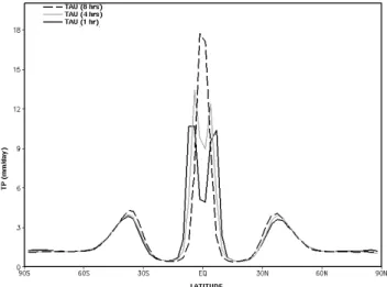
rain-Fig. 1.Zonal averaged time mean total precipitation (TP) with three different TAUs, i.e. TAU (1 h), TAU (4 h), and TAU (8 h). TAU stands for convective relaxation time scale.

fall and TRMM rainfall) for the evaluation, verification, and performance testing.

4 Results of numerical experiments

4.1 Partitioning between precipitation components

(4)

1830 S. K. Mishra and J. Srinivasan: Sensitivity of simulated precipitation to changes in TAU

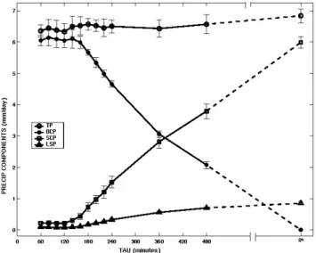
Fig. 2. Area averaged, time mean total precipitation (TP) and its various components (DCP, SCP and, LSP) versus TAU for the re-gion (0◦E to 360◦E and 12.5◦S to 12.5◦N). Points showed adja-cent to the right margin represent TAU =∞. The error bars show the respective standard deviation in time about the time mean val-ues. Notations: TP for total precipitation, DCP for deep convective precipitation, SCP for shallow convective precipitation, and LSP for large-scale precipitation (also called as stratiform precipitation).

4.2 Computation of deep convective precipitation

The closure for the ZM scheme is based on the budget equa-tion for CAPE. This budget equaequa-tion may be written as:

∂A/∂t= −MbF+G (2)

Where,Arepresents CAPE,Grepresents the large-scale pro-duction of CAPE by the grid scale dynamics, and −MbF

represents the sub-grid scale CAPE consumption by the pa-rameterized deep convection. Mbrepresents the cloud base

mass flux, andF represents the rate at which cumulus clouds consume CAPE per unit cloud base mass flux. The closure used in the scheme, in CAM3, is a diagnostic closure condi-tion, which is as follows:

Mb=A/τ F (3)

where,τ is the convective relaxation time scale. This closure assumes that CAPE is consumed at an exponential rate (1/τ ) by cumulus convection. This may be seen by substituting Eq. (3) in Eq. (2), which will give Eq. (4).

∂A/∂t= −A/τ+G (4)

So, if at t=0, CAPE is A0, in the absence of large-scale

CAPE generation, the solution will be,A=A0exp (−t /τ ),

fort >0. Hence, when the relaxation time scale (hereafter will be referred as TAU) is increased, it will reduce the mag-nitude of cloud base mass flux. This in turn determines the updraft mass flux at every level of the model, by taking the

entrainment and detrainment rate into consideration. Even-tually, updraft mass flux along with cloud liquid water deter-mines the DCP production at every model level, as in Eq. (5).

[DCP]i=C0· [Mu]i· [L]i (5)

where,C0 is the DCP production efficiency parameter,Muis

the updraft mass flux, andLis the cloud liquid water at the i-th level. The vertical integral of [DCP]iover all the model

levels, gives the surface reaching DCP.

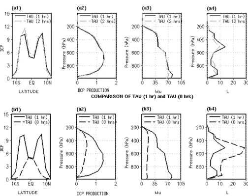
To understand, why change in TAU up to 2 h, there was no impact, 3-cases were chosen (namely, TAU (1 h), TAU (2 h), and TAU (8 h)) for a more detailed investigation. Fig-ure 3 shows surface reaching DCP, vertical structFig-ure of DCP production rate, updraft mass flux, and cloud liquid water. The top panel of the figure shows the comparison between TAU (1 h) and TAU (2 h) and the bottom panel for TAU (1 h) and TAU (8 h). Figure 3a3 shows that updraft mass flux in TAU (1 h) and TAU (2 h)) is almost same at all the model lev-els, except in the layers adjacent to the surface. Figure 3a4 shows the cloud liquid water is almost same in both the cases. Hence, as expected, the DCP production rate (Fig. 3a2) is also found to be same at all the model levels and so is the surface reaching DCP (Fig. 3a1).

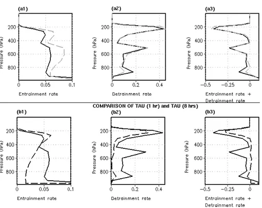
Bottom panel shows that updraft mass flux is lower for TAU (8 h) than TAU (1 h). The cloud liquid water is found to be higher in TAU (8 h). The effect of reduction in updraft mass flux on the production of DCP outweighs that caused by the increase in cloud liquid water and thus resulting in a lower value of DCP production. Figure 4 shows the en-trainment and deen-trainment rates for TAU (1 h), TAU (2 h) and TAU (8 h). Figure 4a3 and (b3) show the net lateral mixing due to the combined effect of entrainment and detrainment. The net lateral mixing is found to be negative in most of the levels in TAU (1 h) and TAU (2 h), which is the reason be-hind the decrease in updraft mass flux with height in these simulations. Whereas in TAU (8 h), the net lateral mixing is nearly zero from the surface up to 300 hPa. This is why, the updraft mass flux does not show an appreciable change with height.

(5)

Fig. 3.Top panel shows the comparison of TAU (1 h) and TAU (2 h), and bottom panel shows the comparison of TAU (1 h) and TAU (8 h).

(a1)and(b1)show the zonal averaged time mean surface reaching DCP (mm/day),(a2)and(b2)show the vertical profile of area (0◦E to 360◦E and 12.5◦S to 12.5◦N) averaged DCP production (kg/kg/day),(a3)and(b3)show the vertical profile of area (0◦E to 360◦E and 12.5◦S to 12.5◦N) averaged updraft mass flux (mb/day), and(a4)and(b4)show the vertical profile of area (0◦E to 360◦E and 12.5◦S to 12.5◦N) averaged cloud water (gram/m2).

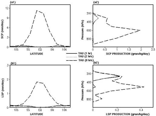
4.3 Shallow convective precipitation and large scale precipitation

Figure 6 shows the impact of TAU on shallow convective precipitation (SCP) and large-scale precipitation (LSP). SCP and LSP are found to be more when TAU is 8 h. Since, there is considerable difference in SCP and LSP in the region 7◦S to 7◦N (see a1 and b1), our analysis will now be confined to this region. When TAU is 1 h, SCP and LSP production was primarily confined to the upper troposphere (see Fig. 6a2 and b2). When TAU is 8 h, a significant enhancement of SCP and LSP is noticed in lower and mid troposphere.

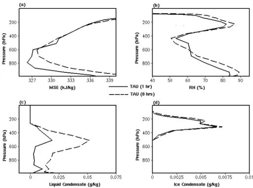
Figure 7 shows the vertical profiles of moist static energy (MSE), relative humidity, liquid condensate and ice conden-sate from TAU (1 h) and TAU (8 h). When TAU is 8 h, the MSE is found to be higher in the lower troposphere and cloud liquid water is higher in lower as well as mid troposphere. Hence, the enhancement of SCP in the lower troposphere is due to increase of both MSE and cloud liquid water. How-ever, increase in SCP in the mid troposphere is due to the in-crease of cloud liquid water alone, as there is not much differ-ence in MSE. Figure 7b shows that RH is more in the lower and upper troposphere, when TAU is higher. As can be seen from Fig. 7c, the liquid condensate is found to be more in the

lower and middle troposphere, when TAU is 8 h, whereas, ice condensate is not significantly different (Fig. 7d). Hence, higher value of LSP in the lower troposphere is due to the increase in RH when TAU is 8 h, whereas, in the middle tro-posphere, the increase in LSP is caused by the increase in liquid condensate.

It is noticed in Fig. 6 that there is no considerable differ-ence between TAU (1 h) and TAU (2 h). This is due to the fact that, DCP was unchanged up to 2 h because of the com-pensation between the decrease of cloud base mass flux and increase of the lateral mixing.

4.4 Temperature and moisture

4.4.1 Vertical structure

(6)

Fig. 4.Top panel shows the comparison of TAU (1 h) and TAU (2 h), and bottom panel shows the comparison of TAU (1 h) and TAU (8 h).

(a1)and(b1)show the vertical profile of area (0◦E to 360◦E and 12.5◦S to 12.5◦N) averaged updraft mass entrainment rate (per day),

(a2)and(b2)show the vertical profile of area (0◦E to 360◦E and 12.5◦S to 12.5◦N) averaged -ve updraft mass detrainment rate, (per day), and(a3)and(b3)show the vertical profile of area (0◦E to 360◦E and 12.5◦S to 12.5◦N) averaged updraft mass entrainment and detrainment rate, (per day).

be responsible for the observed structure of MSE and RH. Similar difference was observed in geopotential height (not shown here), but its contribution to MSE is an order of mag-nitude less than that contributed by temperature and mois-ture.

4.4.2 Heating rates

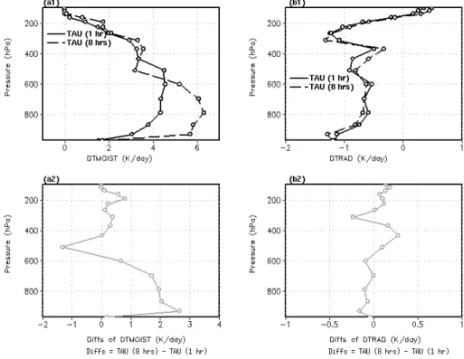
The heating rate due to moist and radiative processes are shown in Fig. 9. Top panel shows the heating rate with TAU (1 h) and TAU (8 h), while the bottom panel shows the differ-ence between them i.e. [TAU (8 h) – TAU (1 h)]. Figure 9a2 indicates that, relatively TAU (8 h) has larger moist heating below 550 hPa and above 250 hPa. In between the above two altitudes it is is lesser than that of TAU (1 h).

However, Radiative processes cause more cooling below 500 hPa and between 350 hPa and 250 hPa, and does the re-verse at all other model layers. Close comparison of Fig. 9a2 and b2 with Fig. 8a revels that, the moist processes are pri-marily responsible for the observed temperature structure, discussed above.

4.4.3 Surface evaporation and large-scale moisture con-vergence

Figure 10a shows the difference in zonally averaged, time mean, surface evaporation between TAU (8 h) and TAU (1 h). Similarly, Fig. 10b shows the difference in the large-scale moisture convergence i.e. (PRECIP – EVP). It is noticed from Fig. 10a that, surface evaporation is more in TAU (8 h) over∼10◦S–10◦N, and beyond 20◦S/N. However, between 10◦S/N to 20◦S/N it is lower than that in TAU (1 h). More-over, over equatorial belt (5◦S–5◦N), the difference is al-most zero. Figure 10b shows that, over 5◦S–5◦N, the large-scale moisture convergence in TAU (8 h) is higher, whereas it is found to be lower in between 5◦_{S/N and 12.5}◦_{S/N. In}

Fig. 8b, it was noticed that, for TAU (8 h), over 7◦_S–7◦_N,

(7)

Fig. 5. Zonal averaged time mean quantities. Top panel shows the comparison of TAU (1 h) and TAU (2 h), and bottom panel shows the comparison of TAU (1 h) and TAU (8 h).(a1)and(b1)show the cloud base mass flux (mb/day),(a2)and(b2)show CAPE (J/Kg),(a3)and

(b3)showF, which is the CAPE consumption rate per unit cloud base mass flux (J/Kg/Mb).

(8)

Fig. 7. Vertical structure of the time mean area averaged quantities over 0◦E to 360◦E and 7◦S to 7◦N with TAU (1 h) and TAU (8 h).

(a)Moist Static Energy (MSE),(b)RH,(c)liquid condensate, and(d)ice condensate.

Fig. 8.Vertical structure of the time mean area averaged quantities over 0◦E to 360◦E and 7◦S to 7◦N with TAU (1 h) and TAU (8 h).(a)T, and(b)Q.

difference between them, i.e. [TAU (8 h) – TAU (1 h)]. It can be noticed from the figure that, more amount of moisture is coming into this region in the lower troposphere, for the TAU (8 h) case. On the other hand, more amount of moisture

(9)

Fig. 9. Top panel shows the vertical structure of the time mean area averaged quantities over 0◦E to 360◦E and 7◦S to 7◦N with TAU (1 h) and TAU (8 h).(a1)Temperature tendency due to moist processes,(b1)temperature tendency due to radiative processes. Bottom panel shows the differences between TAU (8 h) and TAU (1 h).

(10)

Fig. 11. Zonally averaged time mean quantity with TAU (1 h), and TAU (8 h),(a1)wind magnitude at lowest model level (m/s),(a2) per-centage change of magnitude of wind at the lowest model level of TAU (8 h) with respect to TAU (1 h),(b1)dq at lowest model level (g/kg),

(b2)percentage change of dq for TAU (8 h) with respect to TAU (1 h).

Notation: Percentage change of TAU (8 h) with respect to TAU (1 h) = [(TAU (8 h) – TAU (1 h))/TAU (1 h)}·100, dq =QS(TS)– QA.

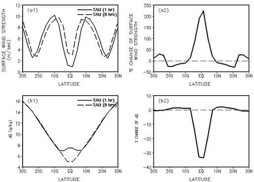
4.4.4 Surface level wind strength and moisture deficit

Figure 11a1 shows the surface level wind strength, and panel (b1) shows the moisture deficit at the 1st model level. In Fig. 11a2 and b2, the corresponding percentage change is shown i.e., [{TAU (8 h) – TAU (1 h)}/TAU (1 h)]·100. Wind strength in TAU (8 h) is found to be higher over 10◦S–10◦N and beyond 20◦S/N, and lower over 10◦S/N and 20◦S/N. On the other hand, the moisture deficit at the 1st model level, is found to be lower with TAU (8 h), between 10◦S–10◦N. A closer look at Fig. 10a and Fig. 11a2 and b2, reveals that the observed surface evaporation profile is due to the combined effect of wind strength and moisture deficit at the 1st model level (dq). However, the surface wind strength is found to be the primary cause, for the enhancement of evaporation over 10◦_S–10◦_{N, which in turn gets transported into 7}◦_S–7◦_N,

by the lateral moisture convergence and causes higher spe-cific humidity in that region.

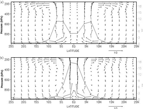
4.5 Large scale circulation

4.5.1 Meridional cell

Time mean, zonally averaged, meridional circulation is shown in Fig. 12a and b, respectively for TAU (1 h) and TAU (8 h). In the background of these plots, zonally averaged time mean total surface precipitation is also shown. The position of the ITCZ and position of the strongest ascent are found to

coincide at the same latitudes. The notable differences be-tween the two cases i.e., TAU (1 h) and TAU (8 h) are the following: in TAU (1 h) the circulation over the equatorial belt is weak, whereas in TAU (8 h) circulation over the same region becomes strong. The rising limb of Hadley cell shifts towards the equator in TAU (8 h), associated with strong sur-face winds over the equatorial belts. This strengthening of the circulation, in turn, leads to an increase in the moisture convergence into the equatorial region.

4.5.2 Vertical velocity

(11)

Fig. 12.Zonally averaged time mean meridional circulation (vector arrows: v; 50xw) and total precipitation (grey line) for(a)TAU (1 h), and(b)TAU (8 h).

(12)

Fig. 14. Vertical distribution of the net precipitation production from each component of the total precipitation. Zonally averaged time mean values are shown. Unit of all the quantities are same and in kg/kg/day. Notation: DCP represents the deep convective precipitation, which is computed by deep convective precipitation scheme. SCP represents the shallow convective precipitation, which is computed by shallow convective precipitation scheme. LSP represents the large-scale precipitation, which is computed by large-scale precipitation scheme. Shading indicates (-)ve values i.e. re-evaporation of precipitating precipitation and cloud liquid water.

Fig. 15. Time evolution of area (12◦S to 12◦N and 0◦E to 360◦E) averaged quantities for integration with TAU (1 h) and TAU (8 h).

(13)

Fig. 16. Time evolution of area (12◦S to 12◦N and 0◦E to 360◦E) averaged quantities. Shown quantities are normalized against their maximum values.(a)TAU (1 h), and(b)TAU (8 h).

Fig. 17.Area averaged (0◦E to 360◦E and 12.5◦S to 12.5◦N), time mean (all months of 10 years) quantities for TAU (1 h) and TAU (8 h).

(14)

Fig. 18. Area averaged (0◦E to 360◦E and 30◦S to 30◦N), time mean (all months of 10 years) quantities for TAU (1 h) and TAU (8 h).

(a)TP, in this plot,(b)deep convective precipitation,(c)shallow convective precipitation,(d)large scale precipitation,(e)EVP,(f)PRECIP – EVP,(g)magnitude of wind at 1st model level,(h)specific humidity at the 1st model level, and(i)CAPE.

the strength of maximum omega. The maximum omega in TAU (1 h) is−0.08 to−0.09 Pa/s, whereas, in TAU (8 h), it is−0.15 Pa/s (see Figs. 4.16a1, and a2).

Figure 13b1 and b2 shows the latitude-height section of the heating rate due to the moist processes, for both the cases. The background gray shading indicates the negative heating due to the evaporation of falling precipitation and melting of the precipitating ice. In TAU (1 h), the primary heating occurs in the upper troposphere, and the secondary in the lower troposphere, whereas, in TAU (8 h), the reverse is true. Besides heating due to moist processes, there are some other heating terms in the model equations, e.g., solar radia-tion, long wave radiaradia-tion, diffusion and KE dissiparadia-tion, and temperature advection, which are not shown here. However, the moist heating is found to be the most important term and largely resembles the structure of omega. Hence, it can be inferred that the structure of omega is primarily governed by the distribution of moist heating.

4.5.3 Vertical distribution of precipitation production

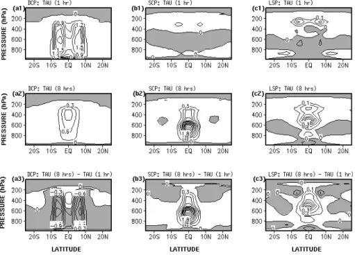
Moist heating comprises of the heating due to DCP, SCP and LSP. Moreover, it also includes the negative heating due to re-evaporation and the (±)ve heating associated with the freezing/melting of falling precipitation. In Fig. 14 the ver-tical distribution of the aforementioned precipitation compo-nents are shown individually. With increase of TAU, the

fol-lowing can be noted from the figure: (1) DCP is decreasing largely throughout the troposphere, (2) SCP is increasing sig-nificantly in the lower- and mid-troposphere, and (3) LSP is increasing in the mid-troposphere. It is also noteworthy that, the magnitude of SCP is approximately one order higher than LSP.

In TAU (1 h), the evaporation of shallow and large scale precipitation (see Fig. 14b1 and c1, respectively) does oc-cur in the lower mid-troposphere, which is the reason be-hind the occurrence of primary peak in heating in the up-per troposphere, and the bi-modal heating structure. In TAU (8 h), most of the precipitation occurs in the lower to mid troposphere by shallow convection (see Fig. 14b2). A small amount of low-level evaporation of large-scale precipitation is noticed in TAU (8 h), which is adjacent to the surface. 4.6 Evolution during spin-up

(15)

Fig. 19.Vertical profile of the difference of the area averaged, time mean, quantities between TAU (8 h) and TAU (1 h), at the raining points. grid points where the total precipitation is more than 1 mm/day are considered as the raining points. Top panel for the deep tropics (0◦E to 360◦E and 12.5◦S to 12.5◦N) and bottom panel for the whole tropics (0◦E to 360◦E and 30◦S to 30◦N).(a1)and(a2)RH difference (%),(b1)and(b2)specific humidity difference (gram/kg),(c1)and(c2)atmospheric temperature difference (◦C). Time mean is calculated by averaging over all the months of 10 years.

evolution of cloud base mass flux, DCP, SCP, CAPE, CAPE consumption rate per unit cloud base mass flux, and LSP, has been shown. Each of the variables shown is found to reach a quasi-steady state within the 96th hour of model integration. From Fig. 15a and c, respectively, it can be seen that, at timet=0 h, there is a difference in cloud base mass flux and DCP, whereas all other variables shown in the figure are same in both the cases. Subsequently, difference in all other variables started showing up, which was seen to grow in time and arrive at their equilibrium level after a few hours of model integration. In Sect. 4.2, the computation of DCP has been illustrated, where Eq. (3) determines the cloud base mass flux. At timet=0 h, CAPE and CAPE consumption rate were same (see Fig. 15b and d), so higher TAU leads to lower cloud base mass flux. Equation (5) determines the DCP, which depends upon C0, updraft mass flux, and cloud liquid water. C0 is a constant parameter and same for both the simulations, and cloud liquid water was also found to be same at time t=0 h (not shown here). Updraft mass flux depends upon cloud base mass flux and lateral mixing due to entrainment and detrainment. We observed at timet=0 that, the lateral mixing is same for both the cases. However, cloud base mass flux is lower in TAU (8 h), which leads to a lower updraft mass flux. A lower value of updraft mass flux, in turn leads to lower DCP. Since convective precipitation consumes

CAPE, decrease in DCP results in increase of CAPE (see Fig. 15b), which in turn increases the DCP, and CAPE con-sumption rate (see Fig. 15c and d). This process continues till a quasi-steady state is reached, which happens at around the 96th hour (see Fig. 15f). During this time, SCP and LSP also increase, because of the increase in the instability of the atmosphere (measured in terms of CAPE).

Figure 16 shows the evolution of the normalized DCP, SCP, LSP, and CAPE to illustrate the lead-lag between them. Top panel (Fig. 16a) is for TAU (1 h), and the bottom panel (Fig. 16b) is for TAU (8 h). As discussed above, TAU (1 h) does not show any major change, which is because of the fact that, it is the continuation of the previous run from where the initial conditions were extracted. However, the simulation with TAU (8 h) shows an increase in CAPE followed by an increase in DCP, followed by an increase in SCP and then an increase in LSP.

4.7 Actual-planet simulations

(16)

Fig. 20. Area averaged (0◦E to 360◦E and 20◦S to 20◦N), time mean (all months) deep convective precipitation fraction from ob-servation (PR), TAU (1 h) and TAU (8 h).

integrated for 10 years with the climatological SST, and for 10 years with the observed SST, with TAU (1 h) and TAU (8 h).

4.7.1 Area integrated precipitation

Monthly data of 10 years from the climatological SST sim-ulations were analyzed to address the impact of TAU on the area-integrated precipitation. Figure 17 shows the impact on precipitation and its associated variables in the deep tropics (12.5◦S to 12.5◦N). From this figure it is seen that TP is largely same, the change being less than 2% of the mean TP (see Fig. 17a). DCP is found to decrease (see Fig. 17b), and SCP and LSP are found to increase with increase in TAU (see Figs. 17c, d). So, it is inferred that TP is insensitive to TAU due to the compensation between the three components of precipitation. Figure 17e shows that, there is an increase in evaporation over the region. Hence large-scale convergence [PRECIP-EVP] is reduced (see Fig. 17f). The increase in evaporation is found to be due to the enhancement in wind strength at 1st model level (see Fig. 17g). Surface evapora-tion is a funcevapora-tion of wind strength and humidity. The specific humidity is higher at the 1st model level (see plot h), thus reducing the moisture deficit. Hence, it is inferred that the increase in evaporation is due to the increase in wind strength at the 1st model level. Figure 17i shows that increase in TAU leads to increase in CAPE. This finding is similar to those found in aqua-planet simulations.

Figure 18 shows the response of the above-discussed vari-ables in the whole tropics (0◦E to 360◦E and 30◦S to 30◦N). It is noticed that, DCP is decreasing (see plot b), and SCP and LSP are increasing (see Fig. 18c and d), with increase in TAU. However, TP is found to decrease by ∼5% (see

Fig. 18a). Evaporation is found to decrease (see Fig. 18e), whereas, wind strength at the 1st model level is found to in-crease (see plot g). Figure 18h shows that specific humidity in the 1st model level is increasing, which means reduction in the moisture deficit at the 1st model level. Hence, it is inferred that, the response of evaporation is due to the dom-inance of the response of specific humidity over the wind strength at the 1st model level. Since, in the deep trop-ics there is an enhancement of evaporation, it could be be-cause of the opposite response in the rest of the tropics (from 12.5◦N/S to 30◦N/S). Figure 18f shows the enhancement in the large-scale moisture divergence. The increase in CAPE with increase of TAU can be seen from Fig. 18i.

Figure 19 shows the vertical profile of the difference in RH, Q, andT, for deep tropics (in top panel), and for the whole tropics (bottom panel). Increase of TAU leads to in-crease in RH throughout the atmosphere (see Fig. 19a1 and 19a2). Specific humidity (Q), is found to increase below 500 hPa, (see plot b1 and b2). Temperature (T) is noticed to have increased in the lower (below 850 hPa), and upper (200–100 hPa) troposphere, whereas, in between it gets re-duced with increase in TAU. So, the increase in RH in the lower troposphere is attributable to the increase inQ, but in the middle troposphere, it is primarily attributable to the de-crease in T. In the upper troposphere, the increase in RH is due to the increase inQ, (not shown here). However, an exception is plot (a2), which shows a slight decrease of RH between 100 to 200 hPa, which is because of the dominant ef-fect of increase in temperature (see Fig. 19c2) over the small increase inQ(see Fig. 19b2) at those levels.

Rasch et al. (2006) showed that the proportion of precipi-tation components in CAM3 is not satisfactorily simulated, though the simulated total precipitation is in close agree-ment with the observation. We noticed that TAU affects the proportion of the precipitation components, by keeping the TP by and large the same. In Fig. 20, the fraction of deep convective precipitation is shown from observation (TRMM Precipitation Radar), TAU (1 h) and TAU (8 h). TRMM product 2A23 places the majority of the shallow convec-tive clouds in the stratiform subcategory (Schumacher and Houze, 2003). So, to compare with the TRMM data, we use similar classification of the TP i.e. deep convective and re-maining as stratiform. Figure 20 shows that, in observation the DCP is around 40% whereas in TAU (1 h) it is around 90%. This is in agreement with the results shown by Rasch et al. (2006). However, in TAU (8 h), proportion of DCP is seen to be around 50%, which is very close to the observa-tion.

4.7.2 Seasonal mean simulation

(17)

Fig. 21.Climatological mean DJF precipitation (mm/day) for(a)TAU (1 h),(b)TAU (8 h),(c)CMAP,(d)[TAU (8 h) – TAU (1 h)],(e)[TAU (1 h) – CMAP], and(f)[TAU (8 h) – CMAP]. The climatological mean is derived from 10 years (1979 to 1988).

(18)

Fig. 23.Difference in the Climatologically mean precipitation (mm/day) between TAU (8 h) and TAU (1 h). The left panel is for DJF and the right panel for JJA.(a)and(b)Total precipitation,(c)and(d)Convective precipitation, and(e)and(f)Large-scale precipitation. The climatological mean is derived from 10 years (1979 to 1988).

From Fig. 21a, it is noticed that, the control simulation successfully captures many of the observed features during Northern Hemisphere winter, e.g., south Pacific and south Atlantic convergence zones, precipitation minima over the sub-tropics of the eastern parts of the oceans of both the hemispheres. Similarly Fig. 22a shows that, the control sim-ulation captures the broad features of Northern Hemisphere summer e.g., precipitation maxima along 10◦N, strong pre-cipitation over western Pacific, prepre-cipitation over eastern Pa-cific, and precipitation minima over the sub-tropical eastern parts of the oceans in both the hemispheres. These are found to be consistent with the previous studies e.g., Hurrell et al. (2006), Rasch et al. (2006), Hack et al. (2006), Collins et al. (2006), and Meehl et al. (2006).

However, there do exist many biases (Hurrell et al., 2006). During northern winter, the precipitation over the south of the equator between 60◦E to 120◦W is underestimated, and over tropical Africa, northern Australia, and north of the equator over the western Pacific, it is overestimated. Similarly, dur-ing northern summer, over the equatorial zone of western, eastern, and central Pacific, and eastern and head of the Bay of Bengal, the model underestimates the precipitation. Over Saudi Arabia, western Indian Ocean, western Arabian sea, and western part of south Pacific, the precipitation is overes-timated.

From Fig. 21, it was noticed that, increase of TAU leads to increase in precipitation south of the equator between 60◦E to 120◦_{W, and south Pacific convergence zone. On the other}

hand, there is a decrease in precipitation over tropical Africa, northern Australia, and north of the equator over the western Pacific. These changes seem to rectify some of the existing biases of the model. However, along with this, there is also an increase in precipitation over the eastern Pacific, resulting in a positive bias. Since some of the existing biases have been rectified, the pattern correlation is found to be better with TAU (8 h) i.e., from 0.79 it has increased to 0.83 (see bottom of the Fig. 21).

It is noticed from Fig. 22 that increase of TAU increases the precipitation over the equatorial belts of western, eastern, and central Pacific. It also increases the precipitation over the eastern coast and north Bay of Bengal, and over the Indian subcontinent. Over tropical Africa, Saudi Arabia, equatorial Indian ocean, western parts of the south Pacific, the precip-itation decreases with increase of TAU. These changes, rec-tifies some of the aforementioned model biases and improve the pattern correlation coefficient from 0.67 to 0.79.

(19)

S. K. Mishra and J. Srinivasan: Sensitivity of simulated precipitation to changes in TAU 1845 positive biases are rectified by the reduction of the DCP and

the negative biases are rectified by the enhancement of SCP and LSP. However, comparatively the contribution of SCP is much higher than that of LSP.

5 Conclusions

The sensitivity of the simulated precipitation to changes in convective relaxation time scale (TAU) of Zhang and Mc-Farlane (ZM) cumulus scheme in NCAR-Community Atmo-sphere Model version 3 (CAM3) was examined. The inves-tigation was carried out in two modeling frameworks i.e., aqua-planet and actual-planet. A series of numerical experi-ments were conducted in the aqua-planet mode by increasing TAU from 1 h (default value) up to infinity, and its impact on simulated precipitation was examined. The deep convective precipitation (DCP) was found to decrease with an increase in TAU. This leads to an accumulation of convective insta-bility and moisture content in the atmosphere. Consequently, the shallow convective precipitation (SCP) and large-scale precipitation (LSP) intensify and cap the accumulation of convective instability. The decrease in DCP and increase in SCP and LSP, have a compensating effect, and thus the net surface reaching total precipitation (TP) is insensitive to TAU. Comparatively the magnitude of the increase in SCP is one order higher than that of LSP. Thus, it is the enhancement of SCP that primarily compensates the decrease of DCP. The DCP occurs throughout the troposphere, with peak in the up-per levels, whereas SCP mainly occurs in the lower- and mid-troposphere. So, when TAU was increased, DCP decreased throughout the troposphere but SCP increased in the lower and mid-troposphere. Hence, even though the surface reach-ing TP remains same, there is a change in the vertical distri-bution of the total precipitation. As a result, the moist heat-ing increases in the lower and mid troposphere and decreases in the upper troposphere. The vertical velocity intensifies in the lower troposphere and the meridional circulation be-comes stronger.

In order to verify if the effects of TAU on simulated precip-itation in an aqua-planet framework translate to a real-planet, numerical integrations were carried out with actual land-ocean distribution, observed sea surface temperatures con-taining the annually varying seasonal cycle, and fully interac-tive physics. The model was integrated for 10 years (January 1979 to December 1988), with TAU = 1 h in one experiment, and with TAU = 8 h in the other. The seasonal mean pre-cipitation was analyzed and compared with observed values (CMAP). The seasonal mean precipitation with TAU = 8 h was found to be more realistic. In a previous study, we have shown that some of the variability aspects (convectively cou-pled equatorial waves) of simulated climate become more reasonable with TAU = 8 h (Mishra, 2007). However, for val-ues of TAU greater than 8 h, the quality of model simulations was found to deteriorate. Since the current work was

car-ried out with a model spectral resolution of T63 (equivalent grid spacing of∼280 km), it seems that 8 h is the optimum value for 280 km horizontal grid spacing. Future work will focus on determining the optimum value of TAU and its de-pendence on model resolution.

Acknowledgements. The first author (SKM) thanks Sandeep

Sa-hany (of UCLA), Brian Mapes (of Univ. of Miami), and Joe Tribbia (of NCAR) for helpful discussions on the related topics. The en-couragement and support of Henry Tufo (of NCAR) and Ram Nair (of NCAR) is sincerely appreciated. The authors gratefully ac-knowledge the helpful comments and suggestions of the two anony-mous referees and Paolo Michele Ruti (topical editor).

Topical Editor P. M. Ruti thanks two anonymous referees for their help in evaluating this paper.

References

Arakawa, A.: The cumulus parameterization past present, and fu-ture, J. Climate, 17, 2493–2525, 2004.

Betts, A. K.: A new convective adjustment scheme. Part I: Obser-vational and theoretical basis, Q. J. Roy. Meteorol. Soc., 112, 677–692, 1986.

Betts, A. K. and Miller, M. J.: A new convective adjust-ment scheme. Part II: Single column tests using GATE-wave, BOMEX, ATEX, and Arctic Airmass data sets, Q. J. Roy. Me-teorol. Soc., 112, 693–710, 1986.

Boville, B. A. and Bretherton, C. S.: Heating and dissipation in the NCAR community atmosphere model, J. Climate, 16, 3877– 3887, 2003.

Bretherton, C. S., Peters, M. E., and Back, L. E.: Relationships between water vapor path and precipitation over the tropical oceans, J. Climate, 17, 1517–1528, 2004.

Brown, R. G. and Bretherton, C. S.: A test of the strict quasi-equilibrium theory on long time and space scales, J. Atmos. Sci., 54, 624–638, 1997.

Collins, W. D., Rasch, P. J., Eaton, B. E., et al.: Simu-lation of aerosol distributions and radiative forcing for IN-DOEX: Regional climate impacts, J. Geophys. Res., 107, 8028, doi:10.1029/2000JD000032, 2002.

Collins, W. D., Rasch, P. J., Boville, B. A., et al.: Description of the NCAR Community Atmosphere Model (CAM 3.0), NCAR Technical Note, NCAR/TN-464+STR, 226 pp., 2004.

Collins, W. D., Rasch, P. J., Boville, B. A., et al.: The formula-tion and atmospheric simulaformula-tion of the Community Atmosphere Model: CAM3, J. Climate, 19, 2144–2161, 2006.

Frierson, D. M. W.: The Dynamics of Idealized convection scheme on the zonally averaged tropical circulation, J. Atmos. Sci., 64, 1959–1976, 2007.

Gates, W. L.: AMIP: the atmospheric model intercomparsion project, B. Am. Meteorol. Soc., 73, 1962–1970, 1992.

Hack, J. J.: Parameterization of moist convection in the National Center for Atmospheric Research Community Climate Model (CCM2), J. Geophys. Res., 99, 5551–5568, 1994.

(20)

Houze Jr., R. A.: Stratiform precipitation in regions of convection: A meteorological paradox?, B. Am. Meteorol. Soc., 78, 2179– 2196, 1997.

Hurrell, J. W., Hack, J. J., Phillips, A. S., Caron, J., and Yin, J.: The Dynamical Simulation of the Community Atmosphere Model Version 3 (CAM3), J. Climate, 19, 2162–2183, 2006.

Johnson, R. H.: Partitioning tropical heat and moisture budgets into cumulus and mesoscale components: Implication for cumulus parameterization, Mon. Weather Rev., 112, 1590–1601, 1984. Lee, J.-E., Pierrehumbert, R., Swann, A., and Lintner, B. R.:

Sensitivity of stable water isotopic values to convective pa-rameterization schemes, Geophys. Res. Lett., 36, L23801, doi:10.1029/2009GL040880, 2009.

Lin, J. L., Mapes, B. E., Zhang, M., and Newman, M.: Stratiform precipitation, vertical heating profiles, and the Madden-Julian Oscillation, J. Atmos. Sci., 61, 296–309, 2004.

Locatelli, J. D. and Hobbs, P. V.: Fall Speeds and Masses of Solid Precipitation Particles, J. Geophys. Res., 79, 2185–2197, 1974. Lorant, V., McFarlane, N. A., and Scinocca, J. F.: Variability of

pre-cipitation intensity: sensitivity to treatment of moist convection in an RCM and a GCM, Clim. Dynam., 26, 183–200, 2006. Mapes, B. E. and Houze Jr., R. A.: Cloud clusters and

superclus-ters over the oceanic warm pool, Mon. Weather Rev., 121, 1398– 1415, 1993.

Mapes, B. E. and Houze Jr., R. A.: Diabatic divergence profiles in western Pacific mesoscale convective systems, J. Atmos. Sci., 52, 1807–1828, 1995.

Mapes, B. E.: Empirical studies of unobservable parameters, 2001 ECMWF annual seminar course on physical parameterization, 2001.

McFarlane, N. A.: The effect of orographically excited gravity wave drag on the general circulation of the lower stratosphere and tro-posphere, J. Atmos. Sci., 44, 1775–1800, 1987.

Meehl, G. A., Arblaster, J. M., Lawrence, D. M., et al.: Monsoon regimes in the CCSM3, J. Climate, 19, 2482–2495, 2006. Mishra, S. K.: The impact of convective relaxation time on the

simulation of seasonal migration of ITCZ, MJO, and Kelvin waves in CAM3.0 An International Conference: Celebrating the Monsoon, IISc, Bangalore, http://www.image.ucar.edu/∼_saroj/

presentations.html, July 2007.

Mishra. S. K., Srinivasan, J., and Nanjundiah, R. S.: The impact of time step on the intensity of ITCZ in aqua-planet GCM, Mon. Weather Rev., 136, 4077–4091, 2008.

Neale, R. B.: A study of the tropical response in an idealized global circulation, PhD thesis, Department of Meteorology, University of Reading, UK, 1999.

Neale, R. B. and Hoskins, B. J.: A standard test for AGCMs includ-ing their physical parameterizations. I: The proposal, Atmos. Sci. Lett., 1, 101–107, 2000.

Rasch, P. J. and Kristjansson, J. E.: A comparison of the CCM3 model climate using diagnosed and predicted condensate param-eterizations, J. Climate, 11, 1587–1613, 1998.

Rasch, P. J., Stevens, M. J., Ricciardulli, L., et al.: A Character-ization of tropical transient activity in the CAM3 Atmospheric hydrologic cycle, J. Climate, 19, 2222–2242, 2006.

Rayner, N. A., Parker, D. E., Horton, E. B., et al.: Global analyses of sea surface temperature, sea ice, and night marine air temperature since the late nineteenth century, J. Geophys. Res., 108, 4407, doi:10.1029/2002JD002670, 2003.

Reynolds, R. W., Rayner, N. A., Smith, T. M., Stokes, D. C., and Wang, W.: An improved in situ and satellite SST analysis for climate, J. Climate, 15, 1609–1625, 2002.

Ricciardulli, L. and Garcia, R. R.: The excitation of equatorial waves by deep convection in the NCAR community climate model (CCM3), J. Atmos. Sci., 57, 3461–3487, 2000

Sahany, S. and Nanjundiah, R. S.: Impact of convective down-drafts on model simulations: results from aqua-planet integra-tions, Ann. Geophys., 26, 1877–1887, doi:10.5194/angeo-26-1877-2008, 2008.

Sundqvist, H.: Parameterization of condensation and associated clouds in models for weather prediction and general circulation simulation, in Physically-based Modeling and Simulation of Cli-mate and CliCli-mate Change, vol.1, edited by: Schlesinger, M. E., 433–461, Kluwer Academic, 1998.

Williamson, D. L.: Time-split versus process-split coupling of pa-rameterizations and dynamical core, Mon. Weather Rev., 130, 2024–2041, 2002.

Xie, P. and Arkin, P. A.: Global precipitation: a 17-year monthly analysis based on gauge observations, satellite estimates, and nu-merical model outputs, B. Am. Meteorol. Soc., 78, 2539–2558, 1996.

Zhang, G. J. and McFarlane, N. A.: Sensitivity of climate sim-ulations to the parameterization of cumulus convection in the CCGCM, Atmos.-Ocean, 33, 407–446, 1995.