Financially Integrated Emerging
Economy:
The Case of Brazil
Marcelo Kfoury Muinhos Doutor em Economia - Universidade de Cornell e
Pesquisador do Banco Central do Brasil
RESUMO
Este trabalho conduz algumas simulações da regra de Taylor ampliada (com a taxa de câm-bio adicionada). Essas simulações foram feitas também para analisar choques externos em um modelo simples de Metas de Inflação com equações de balança comercial. Em contraste com Ball (2000), quando a taxa de câmbio é incluída na regra de Taylor, a volatilidade do produto aumenta após um choque negativo no fluxo de capitais. Além disso, o paper apre-senta um estudo do pass-through da desvalorização da taxa de câmbio para a inflação con-siderando a mudança recente no regime das taxas de câmbio no Brasil. Estimativas
econométricas foram feitas usando as especificações do pass-through sugeridas por Goldfajn e Werlang (2000).
PALAVRAS-CHAVE
pass-through, flutuação da taxa de câmbio, regra de Taylor
ABSTRACT This paper conducts simulations of the augmented Taylor rule (with an added exchange rate term). It has also been made to analyze the response from external shocks in a simple Infla-tion Targeting model with trade balance equaInfla-tions. In contrast to Ball (2000), when the ex-change rate is included in the Taylor rule, output volatility increases after a negative shock to the capital inflow. The paper also studies the pass-through from the exchange rate devalua-tion to infladevalua-tion considering the recent change in the foreign exchange regime in Brazil. Econometric estimations were performed using the specifications of the pass-through sug-gested by Goldfajn and Werlang (2000)
KEY WORDS pass-through, floating exchange rate, Taylor rule
INTRODUCTION
In recent years, one can observe that an increased number of countries have adopted inflation targeting as their monetary policy regime. Even among emerging markets, this policy regime has been adopted recently in a number of countries such as Chile, Brazil, Poland, and Israel. In the opposite direc-tion, some authors such as Calvo and Reinhart (2000) empirically conclude that emerging countries have a bias against flexible exchange rates that are an important feature of the inflation-targeting framework.
They argue that the reasons for the alleged bias against exchange-rate flexi-bility are in general linked to the high pass-through from the exchange rate to inflation (fear of inflation) and the financial imbalances caused by the high degree of foreign-currency indebtedness of firms in those countries (fear of floating). Ball (2000) doubts the adoption of a purely inflation-tar-geting framework is efficient, unless the monetary policy rule is modified in order to give some role to the exchange rate.
This paper conducts simulations in a simple inflation-targeting model for Brazil that include equations for the trade balance and an augmented Taylor rule (with an added exchange rate term) as suggested by Ball (2000). Those simulations enable us to obtain the response for external shocks. In contrast to Ball (2000), when the exchange rate is included, output volatility increas-es after a negative capital inflow shock.
on the trade balance surplus. Section 4 shows the simulation exercises and the last section concludes the paper.
1. STYLIZED FACTS ABOUT THE LIMITED FLEXIBILITY OF THE EXCHANGE RATE IN EMERGING COUNTRIES
The main reasons that are usually presented as the cause of limited flexibility of exchange rate in emerging market countries are:
• the high degree of pass-through from the exchange rate to inflation; • the financial impact of devaluations on dollar denominated liabilities in
the balance sheet of firms;
• the recessionary impact of major devaluations.
In this section we discuss each of the above arguments and use them to frame the Brazilian experience with a floating exchange rate regime.
The empirical evidence on the limited flexibility of the exchange rate in emerging countries (even in those that defined themselves as free floating) has been discussed in many papers. Calvo and Reinhart (2000) is the main reference on this matter.
Regarding the pass-through, Haussmann, Panizza and Stein (1999) present a table with the estimations of the inflation pass-through for more than 40 countries. The authors estimate a below 5% 12-months pass-through for G-7 countries, and on the other extreme, countries like Mexico, Paraguai and Poland have a pass-through higher than 50%.
these reasons, the pass-through indeed was very low in this single episode, but there is no guarantee that this will be the average pass-through for the Brazilian economy. In other phases of the business cycle and with the ex-change rate closer to the equilibrium level, the pass-through might be high-er. The next section presents some estimations for the pass-through in Brazil.
The second negative consequence of extreme volatility of the exchange rate in emerging markets is the occurrence of financial crises caused by the dollar denominated liabilities of firms. Haussmann, Panizza and Stein (2000) ar-gued that:
“Central Banks of countries unable to borrow in their own
currency will internalize the potential impact of a deprecia-tion due to currency mismatches when carrying out exchange rate and monetary policy.”
Those mismatches are even more dramatic in a financially integrated world, where any rumor of financial problems can generate capital flight that might produce self-fulfilling crises.
The third undesirable impact of the devaluations is the resulting recession. Calvo and Reinhart (2000) show that there is no evidence of expansionary effects of devaluation even in developed economies, anyway the drop in GDP growth is higher in emerging countries than in developed ones. Goldfajn and Olivares (2001) also contributed to the debate about the choice of exchange regime. They gathered stylized facts as following:
They also concluded using a panel that countries more integrated to the in-ternational financial markets and with a weaker current account position are less able to use the exchange rate to respond to external shocks.
Analyzing these stylized facts in regard to the Brazilian recent floating expe-rience, we want to show that exchange rate flexibility is not a major concern for Brazilian policymakers. However, a more careful analysis of the impact of the devaluation on the inflation rate is required including the exchange rate as a policy instrument in the monetary policy rule. The next section presents some empirical evidence of the pass-through in Brazil, and after that, a model including the exchange rate in the Taylor rule and uncovered interest parity depending upon which fundamentals are presented.
2. PASS-THROUGH IN BRAZIL: EMPIRICAL EVIDENCE
All the econometric estimates for the Brazilian experience in this paper are based on two equations presented in Goldfajn and Werlang (2000). Two samples were used and forward-looking terms and instrumental variables were also added to the specifications. In order to choose the best results, some in-and-out-of-sample tests were performed.
The first equation is a standard Phillips curve equation, adding a term for the real exchange rate gap and also for the degree of openness of the econo-my in the standard Phillips curve:
(1) where π is the quarterly IPCA inflation, h is the output gap measured as
GDP minus a linear trend, RER is the real exchange rate gap and OPE is the degree of openness of the economy. The degree of openness is the ratio of the sum of import and export to GDP. The real exchange rate gap is the percentage difference between the actual real exchange rate1 and a
Hodrick-Prescott filter of the real exchange rate.
1 The real exchange rate is the price of one dollar in local currency deflated by domestic CPI and
US PPI.
)
( 1 2 1 3 1 4 1 5 1
1
0 t t t t t t t
t =β +β e −e− +β RER− +βh− +βπ− +βOPE− +u
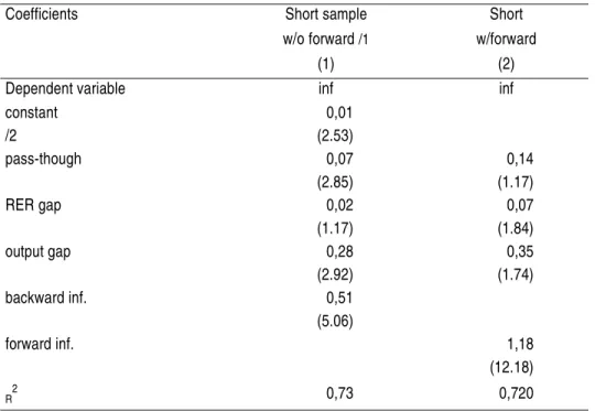
Table 1 presents the results for the 1994:4-2002:2 period (columns (1) and (2)), considering quarterly data. A forward-looking term was also included to cover for inflation expectations in column (2). There are many alterna-tives for modeling expectations. The chosen alternative is to estimate a sim-ple Arma process as the forward-looking term.2 This equation tries to be a
proxy of economic agents expectations. When the forward-looking term is used, there is certainly correlation with the error term, so it is important to use instrumental variables to correct it. The estimations, by a two-stage least squared using as instrument the lagged exogenous variable,3 are presented
in column (2) of Table 1.
TABLE 1 - LINEAR PHILLIPS
/1 without forward-looking term and sample from 1994:4 to 2002:2. /2 t statistics in parentheses
2 An Arma(2,1) for inflation was used as a proxy for the agent's expectations.
Coefficients Short sample Short
w/o forward /1 w/forward
(1) (2)
Dependent variable inf inf
constant 0,01
/2 (2.53)
pass-though 0,07 0,14
(2.85) (1.17)
RER gap 0,02 0,07
(1.17) (1.84)
output gap 0,28 0,35
(2.92) (1.74)
backward inf. 0,51
(5.06)
forward inf. 1,18
(12.18)
The pass-through coefficient is robust for the estimation without forward-looking term. The contemporaneous value is around 10% and is compara-ble to the Goldfajn and Werlang (2000) estimate for the 3-month pass-through. However, it is smaller than the 19.9% value for the America re-gion and similar to the European number. The output gap coefficient is around 30% and greater than in Goldfajn and Werlang (2000) which is lower (0.015). The deviation of the real exchange rate from the equilibrium value is not significant in any model. The same thing happened with the de-gree of openness then it was excluded from the equation in Table 1.
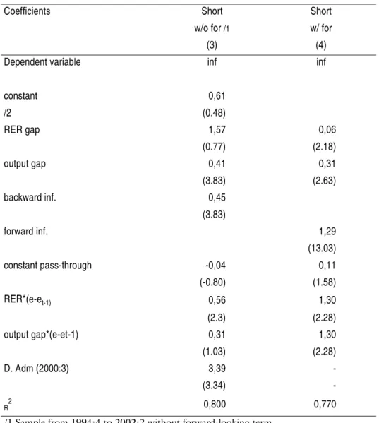
The second equation presented in Goldfajn and Werlang (2000) is a non-linear equation. As explained above, the pass-through is positively related to the output gap, the initial inflation rate and the degree of openness and with the real exchange rate misalignment from its equilibrium.
(2) where
Table 2 contains the results for the non-linear equation. Column (4) con-tains a forward-looking term.4 In the non-linear Phillips curve, instrumental
variables were the exogenous lagged variables.5 The coefficient for the initial
inflation was not significant in any specification and the coefficient for the real exchange rate gap was only significant for the estimation (4). The con-stant terms inside the pass-through (β6) in Table 2 (columns (4) and (5))
are not comparable to the ones reported in Table 1 and they are not signifi-cant at conventional levels.
The output gap* is significant only in (4) and in both
specificati-ons they have the expected sign. In the recession phase of the business cycle the pass-through is smaller and then the sign should have been positive. The
sign and the magnitude6 of the real exchange rate gap are in line with
Gol-4 The same specification for the Arma process.
5 The instrument list: constant, RER gap(-3), inf(-1), infarma(-1) pass-though(-1), d adm (-1,(2000:3)), (RER*(e-et-1)(-3)), (output gap*(e-et-1)(-3))
6 The value of the cross term RER*Ê after 12 months in Goldfajn &Werlang (2000) is 0.67 and highly significant.
)
( 1 2 1 3 1 4 1 5 1
1
0 t t t t t t t
t =β +β e −e− +β RER− +β h− +β π − +β OPE− +u
π
1 10
1 9 1 8 1 7
6
1 = β +β RERt− +β ht− +β πt− +β OPEt− β
)
dfajn and Werlang (2000). The intuition behind this is that because exchange was overvalued pass-through is smaller, meaning room for a correction in
relative prices (tradable & non-tradable). The cross term *
is not important statically in the estimations and it is excluded in (4).
TABLE 2 - NON-LINEAR PHILLIPS
Coefficients Short Short
w/o for /1 w/ for
(3) (4)
Dependent variable inf inf
constant 0,61
/2 (0.48)
RER gap 1,57 0,06
(0.77) (2.18)
output gap 0,41 0,31
(3.83) (2.63)
backward inf. 0,45
(3.83)
forward inf. 1,29
(13.03)
constant pass-through -0,04 0,11
(-0.80) (1.58)
RER*(e-et-1) 0,56 1,30
(2.3) (2.28)
output gap*(e-et-1) 0,31 1,30
(1.03) (2.28)
D. Adm (2000:3) 3,39
-(3.34)
-R2 0,800 0,770
/1 Sample from 1994:4 to 2002:2 without forward-looking term. /2 t statistics in parentheses.
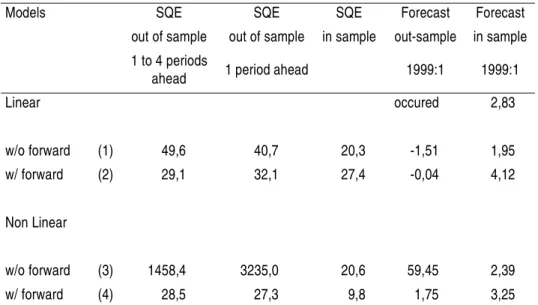
Table 3 presents in-sample and out-of-sample performance tests for the four different specifications. The first two columns are the out-of-sample sum of squared errors (SQE) from 1998:1 to 2002:2.7 The first is the average of
the one to four-steps ahead forecasts compared to the actual inflation out-come and the second is only the one-step ahead forecast. The out-of-sample results are robust with the forward-looking specifications getting better per-formance. The in-sample test the non-linear specification with forward looking term is also the best one, but the specification (3) is not the worst any more, because its in-sample forecast for 1999:1 is not that bad as the out-of-sample ones. The unique exception for out-of-sample forecast for this quarter is specification (4) the non-linear with a forward-looking term. However all models present good results for the in sample forecast in this quarter.
TABLE 3 - PERFORMANCE OF DIFFERENT SPECIFICATIONS
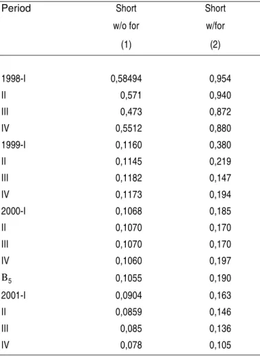
Table 4 shows the evolution of the pass-through when the sample is expand-ed.8 Before 1999:1, the contemporaneous pass-through coefficient is higher
than 50% for the short-sample specifications. This is the explanation for
7 The SQE test is a rolling window with a sample starting in 1994:4 and adding one more obser-vation. In each sample is computed the squared error for the one-step ahead forecast and the average of the one to four step ahead forecasts.
Models SQE SQE SQE Forecast Forecast
out of sample out of sample in sample out-sample in sample
1 to 4 periods
ahead 1 period ahead 1999:1 1999:1
Linear occured 2,83
w/o forward (1) 49,6 40,7 20,3 -1,51 1,95
w/ forward (2) 29,1 32,1 27,4 -0,04 4,12
Non Linear
w/o forward (3) 1458,4 3235,0 20,6 59,45 2,39
w/ forward (4) 28,5 27,3 9,8 1,75 3,25
the enormous out-of sample forecast. After the floating the pass-through reduces steadily for the first two columns.
TABLE 4 - PASS-THROUGH ADJUSTMENTS
In the simulation part of the paper, the chosen specifications were number (2) (the short sample linear model with forward looking expectations), which is the most standard, but with the long run rigidity in nominal vari-ables as explained below and also number (4), which has the coefficient for the cross term output gap and exchange rate difference with the expected sign.
Period Short Short
w/o for w/for
(1) (2)
1998-I 0,58494 0,954
II 0,571 0,940
III 0,473 0,872
IV 0,5512 0,880
1999-I 0,1160 0,380
II 0,1145 0,219
III 0,1182 0,147
IV 0,1173 0,194
2000-I 0,1068 0,185
II 0,1070 0,170
III 0,1070 0,170
IV 0,1060 0,197
Β5 0,1055 0,190
2001-I 0,0904 0,163
II 0,0859 0,146
III 0,085 0,136
3. A SIMPLE MODEL WITH TRADE BALANCE
In order to test for the role of the exchange rate as part of the monetary pol-icy rule, we have to present a complete small inflation-targeting model, which includes an equilibrium condition for the external sector in order to define the exchange rate behavior.
The IS equation is very simple. The aggregate demand only depends on it-self with a lag, on the lagged real interest rate and on the real exchange rate. (3) Where h is the log of the output gap based on a linear trend, θ is the real
exchange rate, i is Selic rate, π is consumer price inflation, and u is the
de-mand disturbance.
The Phillips equation is compatible with any open economy Keynesian model with the restriction of long-term nominal neutrality, which means a vertical Phillips equation in the long run. The econometric estimations in the previous section have not included this restriction in order to be compa-rable with Goldfajn and Werlang (2000). This restriction implies that the coefficients associated with the nominal variables should sum up to 1. Specifications (2) and (4) of the previous sections are used with the restric-tion explained above.
(4) Where is the aggregate supply disturbance and (et – et-1) is the first
differ-ence of nominal exchange rate.
In the appendix one can see the calibrated coefficients for IS equation and for the Phillips curve.
The next equation is a Taylor Rule. However, following Ball (2000) and Mishkin (2000), we add an exchange rate term to the standard rule. In his paper Policy Rules and External Shocks Ball reckons that policy rules used in
closed economies do not fit well for countries that are more sensitive to ex-t
t t
t t
t a a h a i a u
h+1 = 10 + 11 + 12( −π )+ 13θ +
t t t
t t
t t
t a π E a a π a e e a h ε
π = 21 −1+ [(1− 21− 22) +1]+ 22( − −1)+ 24 −1+
ternal shocks. In open economies, such rules should be modified to include the exchange rate. Hence, he suggested a modification in the Taylor rule so that the exchange rate is also included as an instrument in the left-hand side, which is called the Monetary Condition Index (MCI). He presents a very simplified model similar in many ways with the model that is presented in this section.
Ball (2000) in page 12 obtained the following result that we will test for the Brazilian case:
“When there is a shock to net foreign investment, an MCI
target keeps output more stable than an interest-rate target.” The rationale is that when the interest rate is kept constant there is a major devaluation of the exchange rate, which raises aggregate output. On the other hand, when the MCI is held constant, there is a smaller devaluation associated with a rise in the interest rate, with opposite effects on aggregate output that might be held constant.
Ball concludes that “stability is also enhanced by including the exchange rate in policy reaction function.”
In his recent paper Mishkin (2000):
“also reinforces the importance of the exchange rate in infla-tion targeting for emerging countries.”
The author suggests:
that the system is capable of withstanding exchange rate sho-cks.”
If Central Banks are willing to respond strongly to defend the exchange rate, this might hurt the credibility of the monetary policy as the public perceives that protecting the exchange rate is more important than assuring price sta-bility.
The conclusion of the author is that
“One possible way to avoid this problem is for inflation-targe-ting central banks in emerging market countries to adopt a transparent policy of smoothing short-run exchange-rate fluc-tuations that helps mitigate potentially destabilizing effects of abrupt exchange rate changes while making it clear to the public that they will allow exchange rates to reach their market-determined level over longer horizons.”
Hence, there are two instruments in order to reduce inflation rate and the output gap. We are considering that an appreciation will reduce inflation and the output gap, so the second term of the left-hand side of the equation is negative. We are also considering in the rule the first difference of the nominal exchange rate instead of its level. Therefore, the augmented Taylor rule is:
(5) When ω is set equal to one, it is again a standard Taylor rule.
The determination of exchange rate is based on the UIP with fundamentals, in line with Muinhos, Freitas and Araujo (2000), as stated in equation (6). In order to estimate the exchange rate path, however, it is necessary to an-chor the exchange rate at some point in the future. An alternative to achieve this result is to assume that at period t+K the nominal exchange rate will be consistent with a constant current account/GDP ratio. For each period be-tween t and t+K, the nominal exchange rate will move according to the in-terest rate differential corrected by the risk premium, as predicted by the
1 33 1 32 *
1 31
30 ( )
) 1
( − = + − − 1 + − + −
− t t − t t
t e a a a h a i
i ω π πt
UIP hypothesis. Therefore, the following 2 equations determine the ex-change rate path:
, for n < k (6)
(7) where θ is the expected real exchange rate compatible with a constant
cur-rent account/GDP ratio in the medium run, and xt is an exogenous risk
pre-mium that follows an AR(1) process. The equilibrium equation is:
where BS is the balance of services surplus in real terms, BC is the trade
bal-ance surplus in real terms y is the real GDP and b is a arbitrary current
ac-count/GDP equilibrium ratio, that represents a net capital flow consistent with an equilibrium scenario for the capital account. This ratio b is a source
of external shock, representing different international finance liquidity con-ditions as presented in the simulations. BS is an exogenous variable and BC
is determined by:
(9)9
Where Pj is the price index vector for exported and imported goods. Qj is
the quantitative index for exported and imported goods, which depends on the output gap and the real exchange rate, αs are the weights to transform
the indexes in US$ terms.
All the estimates are done using quarterly data with the sample period initi-ating in 1980. We will report here only the coefficients for the trade bal-ance.
b y BC
BS + )/ =
(
∑
= = 2 1 ) , ( j j jjQ y P
BC α θ
K t f K t K t K t
te p p
E + =θ + − + + +
∑
− = + + + + + =− − − + 1 * ) ( K n j K t t j t j t j t t n tte E i i x Ee
The quantitative index for exports is estimated in level, because we could re-ject the unit root for the series. The estimated equation for exports includ-ing the t-statistics in parentheses is:
(10) Where is the world GDP measure as the log of the world’s import quan-titative index. The sample for the above equation comprises the 1991 to 2000 period. We used instrumental variables to avoid correlation between the contemporaneous regressors and the residual. All other information is in the Annex.
When a unit root test is conducted in the import quantitative quantum in-dex, the null of unit root cannot be rejected. However it is clear that a struc-tural break happened in the early 1990’, due to the opening of the economy in the period, which eliminated the ban on some imports and reducing the average import tariff s. If a dummy variable is inserted in the unit root test, one can reject the unit root hypothesis. Hence the estimated equation for imports is:
(11) where d1993 is a dummy that is zero until 1993:3, 0.5 from then to 1994:3 and one afterwards.
4. SIMULATION RESULTS
For the simulation, the two specifications of the Phillips curve were used: number (2) and number (4). Both are with a forward-looking term for in-flation.
For the Phillips equation (2), two types of shocks were tested. The first is to the current account. Three scenarios were considered. The basic one sup-poses that at the end of 2005 the current account deficit/GDP ratio (net capital flow) will reach 2. The worst scenario anticipates a tightening in the
* t y 1993 22 . 0 . 30 . 0 16 . 0 23 . 0 78 . 0 34 . 0 85 . 2 ) 48 . 3 ( ) 81 , 2 ( ) 13 , 2 ( 1 ) 72 , 13 ( ) 56 , 0
( imp y seasonaldummies dCruzado d
impt= + t− + t − − θt + + +
dCruzado mmies
seasonaldu
yt t
international environment, with only a current account deficit of 1% of GDP being sustainable.
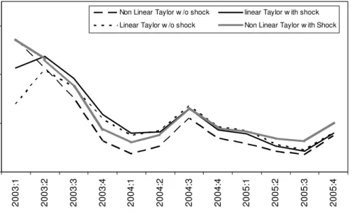
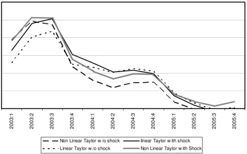
Figure 1 shows the two scenarios for net capital flow. When there is a tight-ening in the financial markets, the exchange rate has to be devalued to as-sure a correction in the trade balance to offset the capital shock. This movement increases inflation and so the interest rate reacts to correct the deviation of inflation from the target. For the same external shock, the non linear Phillips curve brings about very similar results. The only slight differ-ence is the higher level of the output gap in the end of the simulation peri-od for the non-linear Phillips curve. The solid result is the depreciation of the nominal exchange rate in R$ 0,35 per dolar when the equilibrium capi-tal flow shrunk from 2% to 1% of the GDP. Under the shock, the non-lin-ear presents a bit smaller nominal exchange and interest rate.
FIGURE 1 - THE TWO PHILLIPS CURVE WITH AND WITHOUT EX-TERNAL SHOCK
INFLATION
1 2 3 4
20
03
:1
20
03
:2
20
03
:3
20
03
:4
20
04
:1
20
04
:2
20
04
:3
20
04
:4
20
05
:1
20
05
:2
20
05
:3
20
05
:4
Non Linear Taylor w /o shock linear Taylor w ith shock
OUTPUT GAP
NOMINAL EXCHANGE RATE 97,5 98 98,5 99 99,5 100 200 3: 1 200 3: 2 200 3: 3 200 3: 4 200 4: 1 200 4: 2 200 4: 3 200 4: 4 200 5: 1 200 5: 2 200 5: 3 200 5: 4
Non Linear Taylor w /o shock
linear Taylor w ith shock
Linear Taylor w /o shock Non Linear Taylor w ith Shock
2,9 3 3,1 3,2 3,3 3,4 3,5 3,6 3,7 2003: 1 2003: 2 2003: 3 2003: 4 2004: 1 2004: 2 2004: 3 2004: 4 2005: 1 2005: 2 2005: 3 2005: 4
NOMINAL INTEREST RATE
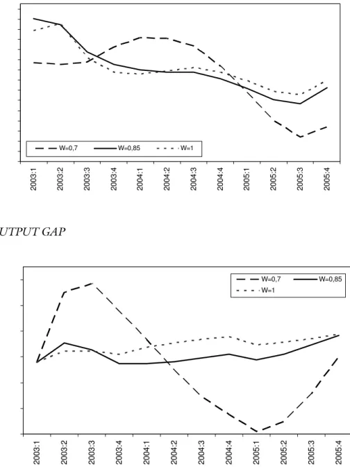
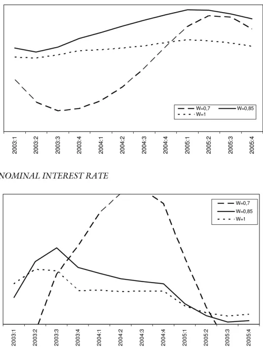
Figure 2 shows different parameterizations of the weight of the exchange rate in the Taylor rule. This weight is not result of any optimization process. It is in line with this kind of rule, when Taylor and Monetary Condition In-dex (MCI) always assume an ad-hoc value. The benchmark is a scenario with no external shocks nor any value for the exchange rate in the Taylor Rule. The first alternative is to set the parameter ω at 0.85, meaning that
the exchange rate is also used as a monetary policy instrument. In the sec-ond alternative, ωis equal to 0.7. As one can see in Figure 2, the third
op-tion brought about an increase of the volatility of the relevant variables.
2003
:1
2003
:2
2003
:3
2003
:4
2004
:1
2004
:2
2004
:3
2004
:4
2005
:1
2005
:2
2005
:3
2005
:4
FIGURE 2 - THE LINEAR PHILLIPS CURVE WITH DIFFERENT WEIGHTS ON EXCHANGE RATE
INFLATION OUTPUT GAP 0,4 0,6 0,8 1 1,2 1,4 1,6 1,8 2 2,2 2,4 2,6 2,8 3 3,2 3,4 200 3: 1 200 3: 2 200 3: 3 200 3: 4 200 4: 1 200 4: 2 200 4: 3 200 4: 4 200 5: 1 200 5: 2 200 5: 3 200 5: 4
W=0,7 W=0,85 W=1
NOMINAL EXCHANGE RATE
NOMINAL INTEREST RATE
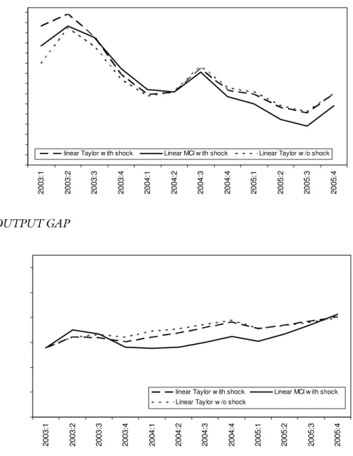
Figure 3 presents the two Taylor rule alternatives when the economy is sub-ject to an external constraint (net capital flow bellow 1% of GDP). In the first alternative no weight is given to the exchange rate. After the shock, the exchange rate and the inflation rate increase less than when the exchange
2003
:1
2003
:2
2003
:3
2003
:4
2004
:1
2004
:2
2004
:3
2004
:4
2005
:1
2005
:2
2005
:3
2005
:4
W=0,7 W=0,85 W=1
2003
:1
2003
:2
2003
:3
2003
:4
2004
:1
2004
:2
2004
:3
2004
:4
2005
:1
2005
:2
2005
:3
2005
:4
in the interest rate results in larger output volatility. The intuition from Ball (2000) does not work in the case of Brazil, because the coefficient for ex-change rate in the IS curve is very small. So the exex-change rate’s devaluation impact on GDP does not offset the impact of the higher interest rate.
FIGURE 3 - TAYLOR RULE, MCI AND EXTERNAL SHOCK (LINEAR)
INFLATION OUTPUT GAP 0,4 0,6 0,8 1 1,2 1,4 1,6 1,8 2 2,2 2,4 2,6 2,8 3 3,2 3,4 20 03: 1 20 03: 2 20 03: 3 20 03: 4 20 04: 1 20 04: 2 20 04: 3 20 04: 4 20 05: 1 20 05: 2 20 05: 3 20 05: 4
linear Taylor w ith shock Linear MCI w ith shock Linear Taylor w /o shock
92 94 96 98 100 102 104 2003: 1 2003: 2 2003: 3 2003: 4 2004: 1 2004: 2 2004: 3 2004: 4 2005: 1 2005: 2 2005: 3 2005: 4
NOMINAL EXCHANGE RATE
NOMINAL INTEREST RATE
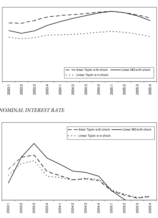
Figure 4 shows how the standard Taylor Rule and the MCI index works for the non-linear Phillips curve under an external shock. The behavior shows the same pattern as in the linear version (Figure3), with a sharper increase
200
3
:1
200
3
:2
200
3
:3
200
3
:4
200
4
:1
200
4
:2
200
4
:3
200
4
:4
200
5
:1
200
5
:2
200
5
:3
200
5
:4
linear Taylor w ith shock Linear MCI w ith shock Linear Taylor w /o shock
2003
:1
2003
:2
2003
:3
2003
:4
2004
:1
2004
:2
2004
:3
2004
:4
2005
:1
2005
:2
2005
:3
2005
:4
linear Taylor w ith shock Linear MCI w ith shock
in the interest rate and a smoother exchange rate with the MCI rule but with a greater sacrifice ratio.
FIGURE 4 - TAYLOR RULE, MCI AND EXTERNAL SHOCK (NON LINEAR) INFLATION OUTPUT GAP 0,4 0,6 0,8 1 1,2 1,4 1,6 1,8 2 2,2 2,4 2,6 2,8 3 3,2 3,4 3,6 3,8 4 20 03 :1 20 03 :2 20 03 :3 20 03 :4 20 04 :1 20 04 :2 20 04 :3 20 04 :4 20 05 :1 20 05 :2 20 05 :3 20 05 :4
linear Taylor w ith supply shock Linear MCI w ith supply shock Linear Taylor w /o shock
90 92 94 96 98 100 102 104 200 3: 1 200 3: 2 200 3: 3 200 3: 4 200 4: 1 200 4: 2 200 4: 3 200 4: 4 200 5: 1 200 5: 2 200 5: 3 200 5: 4
linear Taylor w ith supply shock Linear MCI w ith supply shock
NOMINAL EXCHANGE RATE
NOMINAL INTEREST RATE
One can conclude that when the model is hit by an external shock, a pure Taylor rule will allow a major depreciation and according to Ball, it would increase output, but our model presented more stable output. When a MCI is considered the nominal exchange rate did not depreciate as much but the
3 3,2 3,4 3,6 3,8 4 4,2 4,4 4,6 4,8 5
2003:1 2003:2 2003:3 2003:4 2004:1 2004:2 2004:3 2004:4 2005:1 2005:2 2005:3 2005:4
linear Taylor w ith supply shock Linear MCI w ith supply shock Linear Taylor w /o shock
2003:
1
2003:
2
2003:
3
2003:
4
2004:
1
2004:
2
2004:
3
2004:
4
2005:
1
2005:
2
2005:
3
2005:
4
model suggested a decrease in output in opposite to Ball’s suggestion of a more stable output.
5. FINAL REMARKS
Even considering that exchange rate devaluations in emerging economies may cause high pass-through, financial instability and sluggish output re-coveries, these stylized facts have not been observed in Brazil in the episode of the switching for a floating exchange rate in 1999, at least as the high through. These results presented for Brazil show a smaller pass-through than found by for other American countries. In 2002, after a new wave of exchange rate devaluation, the pass-through seemed to be slighter higher, due to the higher initial inflation, less recessive economy activity and an already depreciated exchange rate. These results in 2002 are again in line with Goldfajn and Werlang (2000).
The non-linear Phillips curve with no forward-looking term does not fit well for the Brazilian data, but the other two with the forward term present consistent results for the two different sample periods. The linear models bring about a major break in the 1999 floating episode what would suggest caution by using those for forecasting purpose.
In the fixed exchange rate regime the entire burden of the shock adjustment is borne by the interest rate. Increasing the volatility of the exchange rate in order to decrease the volatility of the interest rate may be better for the economy.
Why not allow the exchange rate volatility?
• fear of inflation - the results in this paper showed us that Brazilian pass-through has been very low;
• fear of floating - the recent experience proved to us that the balance sheet effects were not so large that they could be safety absorbed in 1999;
• fear of output volatility - the effect of real exchange rate on IS curve was also very small.
The simulations results show that it is better to use a Taylor rule allowing the exchange rate to float using the interest rate only to control inflation.
REFERENCES
BALL, Laurence. Policy rules and external shocks. NBER Working Paper
Series 7910, Cambridge Ma, 2000.
BOGDANSKI, Joel; TOMBINI, Alexandre; WERLANG, Sergio R. C. Implementing inflationtargeting in Brazil. Banco Central do Brasil
Working Paper Series n. 1, Brasília,
CALVO; REINHART. Fear of floating. University of Maryland, 2000.
Mimeografado.
GOLDFAJN, Ilan; OLIVARES, Gino. Can flexible exchange rates still
“work” in financially open economies.G-24 Discussion Paper N. 8,
2001.
GOLDFAJN, Ilan; WERLANG, Sergio R.C. The pass-through from
de-preciation to inflation: a panel study. Banco Central do Brasil
Work-ing Paper Series n. 5, Brasília, 2000.
HAUSSMANN, Ricardo; PANIZZA, Ugo; STEIN Ernesto. Why do
Inter-MISHKIN, Frederic. Inflation targeting in emerging market countries.
NBER Working Paper Series 7618, Cambridge Ma, 2000.
MUINHOS, Marcelo; FREITAS, Paulo; ARAÚJO, Fabio. Uncovered in-terest parity with fundamentals: a Brazilian exchange rate forecast
model. Banco Central do Brasil Working Paper Series n. 19, Brasília,
2000.
RODRICK, Dani. Exchange rate regimes and institutional arrangements in
the shadow of capital flows. Kennedy School of Government, Harvard University, 2000. Mimeografado.
APPENDIX
PARAMETER OF THE PHILLIPS CURVE
PARAMETER OF THE IS CURVE
Phillips Linear Non-Linear
Constant
Pass-Though 0.091181
Real Exchange 0.02703
Output Gap 0.17 0.219254
Pi(t-1) 0.359419 0.308815
Pi(t-2) 0.0924
Pi(t+1) 0.457 0.496774
Pass-Though Constant 0.2652
Real Exchange*Pass-Though. -0.666067
Output Gap*Pass-Though -0.009858
IS Curve Coefficients
Constant 0.0111
Output Gap(t-1) 0.62
Real Interest Rate -0.45
Real Exchange Rate 0
PARAMETER OF THE TAYLOR RULE
The author would like to thank without implications Gil Riella for excellent contributions in run-ning the simulations, Ilan Goldfajn, Pedro Miranda, Edwin Truman, Joaquim Andrade, Maria Beatriz Costa, Thais Porto Ferreira and José Pedro Fachada for reading early drafts of this paper. The views expressed in this work are those of the author and not reflect those of the Banco Central do Brasil or its members.
Email and address: [email protected]. Research Department 9º floor SBS Quadra 3 Bl.B 70074-900 Brasilia DF- Brazil Telefone 61 414 2748 Fax 61 226 0767
Taylor Rule Weights
Inflation 1.5
Output Gap 0.5
Interest t-1 0.6