The Long Term Effects of Bolsa Fam´ılia on
Child Labour and School Enrolment
Marcel Peruffo
∗and Pedro Cavalcanti Ferreira
†May 14, 2015
∗Graduate School of Economics, Funda¸c˜ao Get´ulio Vargas (e-mail: mcperuffo@gmail.com).
Contents
1 Executive Summary 4
2 Introduction 12
3 The Bolsa Fam´ılia Program 14
4 Related Works 15
4.1 Conditional Cash Transfers around the World . . . 19
5 Available Data 20 6 Model 22 6.1 Economic Environment . . . 22
6.2 Preferences . . . 23
6.3 Age Earning Profile . . . 24
6.4 Production Technology . . . 25
6.5 Schooling Technology . . . 25
6.6 The Government . . . 26
6.7 The State Space . . . 26
6.8 The Dynasty Recursive Problem . . . 27
6.8.1 Period 1 . . . 27
6.8.2 Period 2 - Dynasties whose children attended secondary schooling . . . 28
6.8.3 Period 2 - Dynasties whose children did not to attend secondary schooling . . . 30
6.9 Definition of Equilibrium . . . 30
7 Calibration Strategy 33 7.1 The Wage Efficiency Profile . . . 34
7.3 Exogenous Process for productivity . . . 37
7.4 Targeted Moments . . . 38
7.5 Model Outcomes . . . 38
8 Introducing the Bolsa Fam´ılia 39 8.1 Long Term Macroeconomic Effects . . . 41
8.2 Long Term effects on Child Labour . . . 42
8.3 Long Term Effects on Poverty and Inequality . . . 43
8.4 Targeted Families . . . 45
8.5 Welfare . . . 46
1
Executive Summary
• Many works have attempted to evaluate the performance of the Bolsa Fam´ılia, a conditional cash transfer (CCT) program, in reducing poverty and increasing schooling. However, the Bolsa Fam´ılia is a relatively re-cent policy, so the available data is not enough for a definite analysis. This work fills this gap, using computational and simulation tools in order to evaluate the long-term effects of the Brazilian CCT.
• We study the effect of this policy on child labour and school enrolment. By constructing a computational algorithm that simulates the most important features of the Brazilian economy and allows for different policy schedules, we provide an innovative way to evaluate CCTs.
• The main advantages of our approach are:
– The anticipation of the long-term results of such a large-scale
pro-gram, whose macroeconomic impacts are far from negligible.
– The algorithm is versatile, so it allows for the possibility of testing
alternative policy specifications.
– It does not require gathering ex-post data. All data used in the
work come from previously done studies. Hence, spending re-sources on data collecting is not necessary.
own child – this way, generations overlap. In the first period of an in-dividual’s life, decisions related to educational and child labour occur. In the second period, if the individual has attended secondary school she can still choose to go to college, while in the third and four periods she can only work.
• In the simulations we consider our baseline economy as if it were in a pre-CCT environment. We use data from 1997 (mostly from a Brazilian National Homes Sample Survey, PNAD) to validate our model. We then choose to implement a policy scheme to mimic the actual Bolsa Fam´ılia, in terms of family coverage and the program’s total budget. In addition, the transfer requires that the beneficiaries’ children complete (at least) the secondary school.
• The long-term results are extremely positive. Specifically, there’s a huge increase in school enrolment and, as a consequence, in the aggre-gate human capital. Moreover, the transfer reduces by roughly 50% the number of children working.
• As the transfer forces families to enrol their children, in the long-term the majority of the population will (at least) have completed secondary schooling. While in 1997 only 23% of the adults had completed sec-ondary schooling, our simulation suggests that this number increases to 56% after the wide implementation of the new policy. The share of the population with no education reduces from 15% to less than 7%. We also observe a decrease in the number of children who both work and attend school, from 13% to 8%, while the number of children who only work decreases from 9% to 6.5%.
stock increases by 15% due to the fact that, given the better educated labour force, one unit of physical capital is able to produce more than before. For the same reason, the return on physical capital (measured as the interest rate, which grows from 2.6% to 3.0%), increases by 15%. Combined, these three facts show that the macroeconomic impacts of such a transfer policy are substantial.
• There is also an abrupt reduction of poverty - before the CCT imple-mentation, 20.7% of the population lived in such condition. We show that new policy halves this figure. Besides, we observe an increase in welfare, which is proportionally higher for the beneficiaries but is even able to reach the wealthier families.
Sum´
ario Executivo
• Diversos trabalhos realizam avalia¸c˜oes do desempenho do Programa Bolsa Fam´ılia com rela¸c˜ao a diferentes vari´aveis, tais como diminui¸c˜ao da pobreza e aumento da escolaridade. No entanto, esta pol´ıtica ´e relativamente recente, de modo que os dados gerados at´e agora n˜ao s˜ao suficientes para podermos afirmar de maneira definitiva quais s˜ao os impactos do programa. Este trabalho visa preencher esta lacuna, utilizando-se de ferramentas computacionais e de simula¸c˜ao para avaliar impactos de longo prazo do Programa Bolsa Fam´ılia.
• Estudamos os efeitos que essa pol´ıtica possuisobre a escolaridade e so-bre o trabalho infantil. Para isto, provemos uma ferramenta inovadora de avalia¸c˜ao de pol´ıticas condicionais de transferˆencia de renda (CCT), atrav´es da constru¸c˜ao de um algoritmo computacional que simula os principais aspectos da economia e permite a an´alise de diferentes agen-das de pol´ıtica.
• As principais vantagens de nossa abordagem s˜ao:
– Antecipa¸c˜ao dos resultados de longo prazo de um programa social
de larga escala, cujos impactos sobre toda a economia est˜ao longe de serem desprez´ıveis.
– Possibilidade de avalia¸c˜ao de pol´ıticas alternativas – o algoritmo
desenvolvido ´e vers´atil o suficiente para que se possam realizar simula¸c˜oes de diversas naturezas.
– Este trabalho independe da obten¸c˜ao de dados ex-post `a inser¸c˜ao
• A simula¸c˜ao computacional est´a baseada nas t´ecnicas mais avan¸cadas de pesquisa acadˆemica em economia, utilizando-se de mecanismos mi-cro e mami-croeconˆomicos. No modelo, decis˜oes s˜ao tomadas dentro de uma unidade familiar. As escolhas se referem ao n´ıvel de poupan¸ca, ao n´ıvel educacional dos seus filhos, `a oferta de trabalho infantil e ao n´ıvel de consumo.
• Uma unidade familiar consiste de um pai e um filho. Cada indiv´ıduo vive por quatro per´ıodos e, ao fim do quarto per´ıodo, o filho torna-se um adulto, dando origem a um novo filho – ´e o chamado modelo de gera¸c˜oes sobrepostas. No primeiro per´ıodo de vida, ocorrem decis˜oes relacionadas ao n´ıvel de educa¸c˜ao (prim´ario ou secund´ario) e ao tra-balho infantil. No segundo per´ıodo, o indiv´ıduo ainda pode ir para a faculdade e nos demais ele ´e restrito a trabalhar.
• Para efetuar as simula¸c˜oes, consideramos a economia base como se estiv´essemos em um ambiente antes da extensa implementa¸c˜ao do Pro-grama Bolsa Fam´ılia. Para tanto, usamos dados de 1997 (a maioria dos dados foi extra´ıda da Pesquisa Nacional por Amostra em Domic´ılios, PNAD) para validar o modelo, ou seja, para reproduzir os principais aspectos da economia brasileira da ´epoca. Escolhemos ent˜ao um es-quema de transferˆencia de modo que esta beneficie o mesmo n´umero de fam´ılias e represente a mesma fra¸c˜ao do PIB que o programa atual. Al´em disso, ela ´e feita de modo que os filhos dos benefici´arios s˜ao obri-gados a completar a escola secund´aria.
• Como o programa de transferˆencia de renda obriga as fam´ılias a ma-tricular as crian¸cas na escola secund´aria, no longo prazo, a maioria da popula¸c˜ao passa a cursar pelo menos at´e esse n´ıvel. Em n´umeros, en-quanto que em 1997 apenas 23% da popula¸c˜ao adulta possu´ıa escola secund´aria, nossa simula¸c˜ao indica que o Bolsa Fam´ılia aumentaria esse n´umero para 56%. A simula¸c˜ao tamb´em indica uma diminui¸c˜ao no n´umero de adultos sem escolaridade, de 15% para menos de 7%. Por outro lado, a porcentagem de crian¸cas que ao mesmo tempo trabalha e estuda apresenta uma queda de 13% para 8%, enquanto que a fra¸c˜ao dos que trabalham e n˜ao estudam passa de 9% para 6.5%.
• Como conseq¨uˆencia da elevada educa¸c˜ao, a renda m´edia da popula¸c˜ao tem um aumento de mais de 16%. O n´ıvel de capital f´ısico tamb´em apresenta aumento expressivo, de mais de 15%, devido ao fato de que, dada melhor educa¸c˜ao dos trabalhadores, a mesma unidade de capital f´ısico produz ´e capaz de produzir mais do que anteriormente. Como conseq¨uˆencia, o retorno sobre o capital aumenta em 15% (a taxa de juros real passa de 2.6% para 3%). Combinadas, estas trˆes estat´ısticas mostram que os impactos macroeconˆomicos de uma pol´ıtica de trans-ferˆencia de renda s˜ao consider´aveis.
• Nota-se uma brusca diminui¸c˜ao na fra¸c˜ao de fam´ılias pobres da eco-nomia. Antes da implementa¸c˜ao da pol´ıtica, 20.74% da popula¸c˜ao vi-via abaixo da linha de pobreza. Mostramos que o esquema proposto de transferˆencia reduz quase pela metade o n´umero de fam´ılias nesta situa¸c˜ao. Al´em disso, vemos que a implanta¸c˜ao de uma pol´ıtica de transferˆencia de renda gera um aumento de bem-estar proporcional-mente maior para as fam´ılias mais pobres, mas que, ainda assim, h´a ganhos de bem-estar mesmo para as fam´ılias n˜ao benefici´arias.
Abstract
2
Introduction
Malala Yousafzai and Kailash Satyarthi won the 2014 Nobel Peace Prize “for their struggle against the suppression of children and young people and for the right of all children to education”. The girl, the youngest person ever to win the Nobel prize, became famous after sending a letter to BBC explaining the situation of education where she lived, in northwest Pakistan, where the Taliban banned girls from schooling. Kailash’s efforts largely in-fluenced the International Labour Organization to adopt the Convention no. 182, which nowadays consists of the organization’s main guidelines concern-ing the worst forms of child labour1.
Child Labour concerns are appealing. They motivate people and govern-ments to gather resources or to provide specific policies, aimed at reducing child labour and raising school enrolment. The concerns range from child health and safety to human capital accumulation and economic development. For instance, in the Brazilian context, the PETI (Program for the Eradica-tion of Child Labour) offers a cash transfer to families whose children are in working situations. In addition, Brazilian Bolsa Fam´ılia could also have an effect on reducing child labour and inducing school enrolment as, fortunately, many other poverty-reducing policies (de Hoop and Rosati (2013) covers an extensive recent literature on cash transfers and their effects on child labour). The efforts to mitigate child labour appear to be succeeding, since the ILO-IPEC (2013) report suggests that governments, workers and employers organisations, and civil society are on the right track and moving in the right directions. Data corroborate this statement: according to the same report, from 2000 to 2012, the number of children working has fallen from 255 mil-lion to 168 milmil-lion2, which accounts for barely 11% of world’s child (5-17
1
In October 2014, a total of 179 countries have ratified the Convention no.182.
2
year-old) population3.
In this work, we provide a dynamic heterogeneous agent model that in-cludes the most important determinants of child labour and enrolment and then assess the effects of the Brazilian Bolsa Familia, an extensive conditional cash transfer program adopted after 2002. We model a household as a unit consisting of not only a working adult, but also a child, where the trade-off lies in the time allocation of the child, either in leisure, working or investing in human capital.
Our goal is to compare the outcomes generated by different policy incen-tives in stationary equilibria and then assess the groups who are better off and worse off with respect to their previous situations. In addition, we are able to understand differences in aggregate outputs, such as the total hu-man capital accumulation, total child labour, inequality measures and also whether the policy-targeted groups react as the policy-maker expected.
We calibrate the model using Brazilian data. Our results suggest that, in the long-term, the program is successful in increasing school matriculation and reducing child labour. Specifically, with a flat transfer schedule, the new policy raises secondary school enrolment by 30% while the number of working children decrease by more than one third. Also, the model suggests that the program effectively reduces poverty in the whole economy - the introduction of a transfer roughly eradicates poverty among its beneficiaries.
We also perform a counterfactual experiment with a progressive transfer
there are actually 215 million of children working worldwide, with more than half of them being exposed to serious hazards.
3
scheme. In this case, the policy is able to reach the most impoverished fam-ilies. In comparison, with a flat transfer scheme, many families chose not to take the transfer because they would have to accept the conditionality terms. The counterfactual experiment suggests that a progressive transfer scheme that gives more to the poorest is a much more powerful policy. This schedule is able to increase secondary school attendance even more than the flat specification, while it also twice as effective in reducing child labour.
The rest of this paper is organized as follows: section 2 introduces the Bolsa Familia program, section 3 looks at the related literature, section 4 de-scribes some aspects of the data, section 5 presents the model itself, section 6 explains the calibration strategy, section 7 implements the Bolsa Familia and the counterfactual experiment and evaluates the results and section 8 concludes.
3
The Bolsa Fam´ılia Program
In 2004, the ex-president Lula da Silva united four previous transfer pro-grams in order to create the Bolsa Famila, the biggest Brazilian conditional cash transfer program. In 2006, the program had already reached its initial coverage goal - 11 million families (Soares et al. (2009)). In 2009, the gov-ernment authorized its expansion to 12.6 million families. As a result of the program, school registration increased and labour supply did not decrease at all (Soares et al. (2010)). Also, Soares et al. (2006) estimate that the Bolsa Familia was responsible for one fifth of the reduction of the Gini index from 1995 to 2004 (the total decrease was 4.7 points).
per capita income below R$77.00, and the poor families, whose per capita income range from R$77.00 to R$154.00 4. The extremely poor families
re-ceived a monthly “basic benefit” fixed at R$77.00. Also, there’s a monthly variable benefit of R$35.00 for each child from 0 to 15 years old5 (up to 5
children), which is conditional on school registration for children older than 6. There’s also another variable benefit per up to two adolescents (16-17 years old), which is worth R$42.00. Finally, there’s a discretionary benefit, paid to those families who are in the range of extreme poverty. All in all, the average benefit paid in June 2014 was R$167.00 per family per month6.
In december 2012, according to IPEA, the benefit was paid to 13.9 million out of almost 67 million families, with a total of roughly two billion Brazilian reais (an average of R$144.74 per family). Using the data for nominal GDP obtained from the same source (IPEA), we find out that the Bolsa Familia accounted for 0.55% of the GDP in that year.
4
Related Works
Household income directly impacts child labour supply, so, not surpris-ingly, the poorest countries are those where child labour is more persisting. For instance, ILO-IPEC (2013) reports that 30% of Sub-Saharian African children work, a third of which under hazardous conditions. The high inci-dence of child labour among poor households not only is worrying by itself, but also due to its dynamic effects - a working child has a lower performance at school, as extensively reviewed by Orazem and Gunnarsson (2003) - which could ultimately translate into lower future productivity and, thus, wages. As the time invested in acquiring human capital lowers, its accumulation also
4
One Brazilian real was worth roughly $0.3 at the beginning of March/2015.
5
Also given to the families with pregnant mothers. There is also an extra benefit for children ranging from 0-6 months, due to nutritional concerns, which is worth R$35.00.
6
lowers, inducing a kind of intergenerational child labour trap, as emphasized by Baland and Robinson (2000).
Concerns over child labour rely on health and its effects over education, as covered by Dorman (2008). This study provides many examples of works showing that child education and thus human capital accumulation is neg-atively correlated not only with the incidence of child labour, but also with working hours. In addition, school achievement could also be affected by child labour, which ultimately translates into lower wages in the future (Ilahi et al. (2005)).
On the other hand, Dorman (2008) provides broad evidence that child health is negatively affected by working hours. Although very hard to empir-ically assess, the influence of working on child health attracted the attention of the International Labour Organization, who then produced the Conven-tion no. 182.
The incidence of child labour may reflect the inability of households to optimally invest in human capital. This fact is explored in a simple frame-work provided by Lochner and Caucutt (2012) where, when credit constraints problems arise, parents are not able to borrow against their children future earnings. However, empirical works that show the linking between child labour and credit constraints are relatively rare (Edmonds (2008)), due to the unavailability of adequate data. In spite of this difficulty, Beegle et al. (2005), who find out that the availability of collateralizable assets offsets the increase of child labour due to a productivity shock, is an example of such evidence.
Some works try to explicitly model child labour and draw some conclu-sions over welfare and the desirability of its existence. Much of this literature builds on Basu and Van (1998), who also model the household composed of parents and children as the relevant agent in the economy. On the same line, Baland and Robinson (2000) explain that even if parents are fully altruistic, as in our model, (Pareto) inefficient child labour may arise due to market im-perfections. Also, Doepke and Krueger (2006) explore child labour not only under a positive perspective, but also from a normative political-economy approach. They argue that, when market imperfections exist, even though a total ban may be (Pareto) inefficient, it could arise due to political-economic reasons.
Our model elaborates on Krueger and Donohue (2004) and Restuccia and Urrutia (2004), who also construct dynastic overlapping generation models. The first authors calibrate the parameters using US data from 1870, evaluat-ing policies such as a child labour ban, free education and free and mandatory education7. On the other hand, another work by de la Croix and Doepke
(2002) explores, in a framework without physical capital accumulation, how child labour and human capital accumulation interact with fertility and eval-uates benefits of adopting public schooling.
When it comes to evaluating the effects of conditional cash transfers, two works are particularly worth remarking. First, Cespedes (2010) develops a life-cycle model that includes human capital accumulation to evaluate the ef-fects of Mexican PROGRESA, finding that this policy induces human capital accumulation and decreases poverty as a whole. On the other hand, Zilber-man and Berriel (2012) also models the Bolsa Familia transfers in Brazil, though abstracting from human capital and focusing on the financial side, also suggesting that a conditional cash transfer appears to increase welfare.
7
As for the empirical works, there is no lack of this kind of analysis. For instance, a study that reviews the effect of Bolsa Familia in Brazil is Car-doso and Souza (2004). Using data from census they find that the program increased child school matriculation, from 92% to 95%. Moreover, it also changes the work-schooling distribution of children’s endowment of time. Children who previously only worked and children who were previously idle seem to be enrolling after the treatment. On the other hand, child labour remained almost stable as there was an increase in the children that go to school and work both.
A very influential work in this field is Skoufias and Parker (2001), who also explore the effects of Mexican PROGRESA (now renamed Oportunidades). They find evidence that, in response to the new policy, children reallocate their leisure time, for the increase in school registration is lower than the decrease in child labour. This fact is also shown by Ravallion and Wodon (1999) in Bangladesh8. Another research conducted in Costa Rica by Duryea
and Morrison (2004) obtained the same (qualitative) conclusions.
Finally, the last kind of work that evaluates conditional transfers involves structural econometrics. Two works are worth citing. First, Todd and Wolpin (2002) construct a dynamic structural model and validate it, fitting it to real data obtained also from Mexican Oportunidades. Although, as reported by the authors, the analysis does not include general equilibrium effects, on the short term the model was able to provide a policy outcome forecast accu-rately9. In the Brazilian context, Bourguignon et al. (2003) has a humbler
structural estimation, though seeking the perform the same analysis.
8
The Bengali program, the Food-for-Education, provided a non-negligible amount of rice (worth about half the mean income of a poor family), the most important compound of Bengali diet, for children who regularly attended school.
9
4.1
Conditional Cash Transfers around the World
Conditional cash transfers (CCTs) have become widely popular amongst developing countries throughout the nineties and, perhaps surprisingly, even in developed countries. The first CCT program that jumped to the world’s eyes was the MexicanOportunidades, but, in fact, the first experience of this kind took place in Campinas, a city in Brazil, two years prior to PROGRESA implementation (Sedlacek et al. (2000)).
Nowadays, examples of such policies in Latin America are the Costa Rican
Avancemos, Ecuadorian Beca Escolar, Nicaraguan extinctRed de Proteccion
Social, Bengali Food-for-Education, and Chilean Subsidio Unitario Escolar.
In Africa, CCTs were introduced in countries such as Burundi, Burkina Faso, Cˆote d’Ivoire, Cameroon, Ethiopia, Ghana, Guinea, Gambia, Kenya, Mada-gascar, Mozambique, Malawi, Nigeria, Uganda, and Zambia (Nanak Kakwani (2005)). In Asia, the Cambodian Education Sector Support Project, the 4Ps in Philippines, along with the Food-For-Education can be cited. In Europe we can find the Macedonian Conditional Cash Transfer Program and even in the United States a transfer program was launched in New York in 2007, being extinct in 201010.
Such policies, as mentioned, are primarily focused on reducing poverty as a whole. In the context of a dynamic general equilibrium model they relax the non-negativity constraint either on bequests or on asset accumulation. However, only a cash transfer may not be enough to smooth consumption the way the families desire, so instead of allocating the new resource on, say, education (which is arguably desirable by authorities), people use it to
alle-10
viate hunger. The result is an educational trap, with high intergenerational correlation of human capital.
On the other hand, when the targeted households are required to send their children to school, the whole economy may dynamically push into an equilibrium (whose policy is part of) where the aggregate human capital and the marginal returns on capital are high, so the equilibrium output is higher than before. In fact, the greatest virtue of a general equilibrium model is allowing us to understand the interaction of apparently unlinked variables.
5
Available Data
The Pesquisa Nacional por Amostra de Domic´ılios (PNAD), a
Brazil-ian national household sample survey, provides detailed micro-data on each household member occupation. We selected two specific years in order to in-spect data on school enrolment and on child labour11: 1997 and 2011, before
and after the wide implementation of Bolsa Familia.
Before presenting these data, it is important to understand what was happening to the Brazilian economy at the time. The Workers Party, after being elected in 2002, strengthened the existing social programs, and created the Bolsa Familia. Also, the country experienced an impressive economic growth. Between 1997 and 2011, per capita income increased by 30%12.
Meanwhile, the human capital index13 increased by 18%, while school
en-rolment and child labour have moved towards the desired directions. We can see, from table 1, that more children are enrolled in 2011 in comparison to 1997, and less are working. However, this table calls the attention for other correlations. First, children who work are, consistently for all ages and both
11
Unfortunately, there is no data on child labour for children below 10 years-old
12
According to IPEA.
13
periods, less likely to go to school. Second, we can see that there is a higher increase in school enrolment among children who also work, which suggests that families could be reallocating their children’s time (mostly) from leisure into schooling.
Table 2 shows another interesting correlation. First, it makes clear that there has been an increase in enrolment as well as a decrease in working children and idleness14. In addition, we can see that there is a positive
cor-relation between family income and school enrolment. In fact, children who go to school have, on average, a higher family income (excluding their own) when compared to children that work, and this relation holds for both 1997 and 201115.
Both tables 1 and 2 show that there has been, between 1997 and 2011, a negative correlation between per capita income and child labour, a positive correlation between per capita income and school enrolment, and a negative correlation between child labour and school enrolment, all of which consis-tent with the empirical literature.
In the next section, we provide a dynamic heterogeneous agent general equilibrium model containing the main determinants of school enrolment and child labour. Our ultimate goal is to evaluate policy experiments, and we focus on the introduction of a conditional cash transfer scheme.
14
An idle child is defined as a child that neither goes to school nor works.
15
6
Model
6.1
Economic Environment
The economic environment consists of overlapping generations, with time being discrete, and no population growth. Individuals live for four periods, one as a child, one as a young adult and two as adult parents. At the begin-ning of their third period of life, individuals give birth to a child. Thus, each household consists of an adult parent and a child or a young adult. Hence, the dynasty is the relevant agent in this economy. All decisions are jointly taken within the dynasty, so we assume that there is no conflict between its members. Also, an individual dies at the end of the fourth period.
A model period consists of 17 years. However, during his first 10 years of life, an individual can only spend his time in leisure. During the other seven years of childhood he can either work, go to school or stay idle. It is possible to choose between three levels of schooling at this period: no schooling at all, only primary schooling, and secondary schooling. Schooling has not only an explicit cost but also a cost in terms of foregone earnings, which also de-pends on the educational level chosen. On the other hand, at the same time, a young parent of the same dynasty provides all of his endowment of time to the representative firm, in exchange for his wages.
At the end of the first period of his life, a child becomes a young adult and a young parent becomes an old parent. A young adult can either go to college or not (as in Restuccia and Urrutia (2004)), which takes 4.5 years of the individual’s full time and costs a certain amount of resources. The remaining of a young adult’s time is fully devoted to work. The old parent also devotes his full time to work. At the end of this period, a young adult becomes a young parent as the old parent dies. This way, the dynasty con-tinues as generations overlap.
in precautionary savings (which, in the second period, take the form of be-quests). In the first period, a dynasty chooses the child’s level of schooling and the child’s labour supply to the market representative firm. Also, the dynasty chooses the level of physical capital to be taken to the second period. In the second period, beside the asset holdings decision, a young adult that attended secondary schooling is able to choose whether to go to college or not.
In this economy, there’s is only one way to directly transfer resources across time, which is by lending to the representative firm. The representa-tive firm faces no uncertainty, and thus, in the following period, surely pays an interest rate to the lenders.
6.2
Preferences
Here, we divide the dynasty’s life-cycle into two periods. In the first of them, the dynasty consists of a child and a parent living through its third period of life. In the second, it consists of a young adult and of an adult who’s living through its fourth period of life.
Each dynasty seeks to maximize its discounted expected utility. In the first period, dynasties wish to consume but do not wish to send their children to work. Hence, its utility function is:
u1(c, m) =
c1−γ
1−γ
−(φ+I[h′ > h0]φws)m (1)
The first term of the r.h.s represents the perceived utility from household consumption, whilem represents the amount of time a children works.. Also
φ represents the marginal disutility of child labour, while φws represents the
incremental marginal disutility of working and studying both.
utility function is only represented by:
u2(c) =
c1−γ
1−γ
(2)
6.3
Age Earning Profile
The effective units of labour an individual can supply to the market is given by his productivity, which depends on his (relative) human capital and on an exogenous shock.
There are four levels of human capital, so hi ∈ {h0, h1, h2, h3}, which
refer respectively to no schooling, primary schooling, secondary schooling and college. Also, an individual can be affected by his work experience, which is given by ξi(ti, hi), where ti ∈ {1,2,3,4} refers to the individual’s
period of life.
Productivity shocks only affect adult individuals16. Let z
i be the shock
that affects the adult individual of a household i. I assume, as in Seshadri and Lee (2014), that zi follows a log-normal distribution.
log(zi′) =−(1−ρ)σ
2
2 +ρlog(zi) +ǫi, ǫi ∼N(0, σ
2), (3)
where ρ ∈ (0,1). Note that we normalize the unconditional average of this AR(1) process to be −σ2
2, so we have E(z) = 1. Also, the unconditional
variance equals σ2
1−ρ2. There are two underlying assumptions behind this
process. First, the persistence of a the productivity is considered within
household, not within individuals. That is, the productivity of the parent who’s living through his fourth period of life affects the productivity his son will have in the next period the same way the productivity of a parent living through his third period of life affects his productivity during his last period of life. Second, the productivity variance is the same regardless of an
16
individual’s age or education.
We will return to this issue in the calibration section.
6.4
Production Technology
The representative firm has the usual constant returns to scale technology, denoted by:
F(Kt, Lt) =AKtαL1− α
t (4)
WhereKt denotes the aggregate level of capital,Lt the aggregate level of
labour efficiency units and A is the TFP. In this work I consider any type of human capital level (including child labour) as perfect substitutes. The firm pays an interest rate r and wages wfor its inputs.
Since capital depreciates at rateδ, the firm’s problem becomes:
max {Kt,Lt}≥0
AKtαL1t−α−wLt−(r+δ)Kt (5)
The firm’s problem yields the competitive labour and capital prices:
wt=A(1−α)
Kt
Lt α
(6)
and
rt=Aα
Kt
Lt α−1
−δ (7)
6.5
Schooling Technology
In order to invest in human capital accumulation, dynasties are able to send their children and young adults to school. We denote by κ(hi) the cost
of obtaining hi units of human capital.
During the first period, this fraction is strictly increasing in the level of ed-ucation. During the second period, young adults that attend college also forgo a fixed fraction of their time endowment. We will use the function ς(·) and the parameter ̟ to denote the time required to attend a certain level of schooling. More details on this issue will be explored in the calibration section.
6.6
The Government
The government runs a budget balance in each period. Its revenues consist of total income taxes, which I denote (τ). It rebates its revenues either with a conditional transfer (ctr) or with school subsidies. The conditional transfers may be conditioned on (i) school matriculation, which I denote sthr, and (ii) an income threshold, which I denote by ithr. The government is able to define a subsidy schedule, which I denote by S(hi).
We assume throughout this paper that the government is fully credible and its policies are fully observable. Hence, in a steady state equilibrium, which is the type of equilibrium we will be interested in, the policies are constant over time. We also assume that the government policies are fully enforceable at no cost.
6.7
The State Space
The state space of a dynasty who’s going through the first period consists of the bequest it received, denoted by a, the human capital accumulated by the young adult h, and the productivity shock that affects him, z. Let the state space of period one be denoted by x1 ={z, h, a}.
denoting by h) but also the education the young adult has taken in the first period, which I will denote by hc. Also, the parent’s observable shock and
their initial level of asset holdings are considered. We can hence define the state space of the second period dynasty as x2 ={z, h, hc, a}.
6.8
The Dynasty Recursive Problem
6.8.1 Period 1
In the first period, the household’s problem can be defined as:
V1(x1) = max c,m,h′,a′
c1−γ
1−γ
−(φ+I[h′ > h0]φws)m+β X
z′
Prob(z′|z)V2(z′, h, h′, a′)
(8)
subject to:
0≤m+ς(h′)≤m¯ (9)
c+ (1− S(h′))κ(h′) +a′ =a+ (1−τ)[(zξ(3, h) +ξ(1, h′)m)w+ra]+
ctr×I{[(zξ(3, h) +ξ(1, h′)m)w+ra]≤ithr} ×I[h′ ≥sth] (10)
h′ ∈ {h0, h1, h2} (11)
a′ ≥a (12)
m∈[0,m¯], c≥0, (13)
Constraint (9) represents the fraction of endowment of time of a child that can be used for attending school and working (the rest is implicitly allocated into leisure). Equation (10) represents the dynasty’s resource constraint. In the right-hand-side, the expression [(zξ(3, h) +ξ(1, h′)m)w] represents the gross labour income of the family. The first term in the parenthesis,zξ(3, h), represents the efficiency units of labour provided by the adult parent. On the other hand, ξ(1, h′) represents the efficiency units of labour provided by the child. A further explanation of why ξ(·) depends on h′ will be provided in the calibration section.
Constraint (11) represents the human capital investment possibilities in period 1, which are no schooling at all, primary, or secondary schooling, while equation (12) represents the credit constraint. Finally, equations (13) represent time feasibility and consumption non-negativity .
As one can predict, depending on the first period’s level of schooling, the child will have different choice possibilities in the second period. If the child hasn’t attended secondary school, the dynasty cannot invest in his education any more. On the other hand, attending secondary school gives the young adult the possibility to attend college and thus increase his future earnings. For these reasons, two value functions will be defined for the household’s problem in period two.
6.8.2 Period 2 - Dynasties whose children attended secondary
schooling
In the second period, the household whose young adult can still go to college solves:
V2,s(x2s) = max c,g,a′
c1−γ
1−γ
+βX
z′
subject to:
g ∈ {0,1} (15)
h′ =h3g+h2(1−g) (16)
c+g(1− S(h3))κ(h3) +a′ =a+ (1−τ)[(zξ(4, h) +ξ(2, h2)(1−g) +g(1−̟)ξ(2, h3))w+ra]
(17)
a′ ≥a (18)
c≥0, (19)
where x2
s = (z, h, h2, a). Moreover,̟ represents the time required to attend
college, and g equals one if the young adult attends college and 0 otherwise. As before, restrictions (18) and (19) refer respectively to the credit constraint and to the non-negativity of consumption.
Equation (17) represents the household’s resource constraint. In the left-hand-side, (1−S(h3))gκ(h3) represents the net cost of attending college (h3).
In the right-hand-side, [(zξ(4, h) + ξ(2, h2)(1 −g)̟ +g(1−̟)ξ(2, h3))w]
represents the total gross labour income of the dynasty. The term zξ(4, h) represents the efficiency units of labour provided by the adult parent,ξ(2, h2)
represents the total labour efficiency units provided by the young adult who does not attend college, and ξ(2, h3) represents the efficiency units provided
by the young adult who has attended college. Notice that ξ(2, h3) will be
6.8.3 Period 2 - Dynasties whose children did not to attend
sec-ondary schooling
In the second period, the household whose young adult can’t go to college is:
V2,n(x2n) = max c,a′
c1−γ
1−γ
+βX
z′
Prob(z′|z)V1(z′, h′, a′) (20)
subject to:
c+a′ =a+ (1−τ)[(zξ(4, h) +ξ(2, hc))w+ra] (21)
h′ =hc (22)
a′ ≥a (23)
c≥0, (24)
wherex2n = (z, h, hc, a) andhc ∈ {h0, h1}, which, along with (22), states that
the young adult cannot invest any further in human capital. Notice that, in this case, the household’s problem is summarized by only an asset holdings choice, with the actual level of the young adult’s human capital being carried on to the next period.
6.9
Definition of Equilibrium
In this work, we are only interested in stationary recursive competitive equilibria. A stationary recursive competitive equilibrium consists of:
D1 Three groups of functions: (i) {V1, g1c, gh1, gm1 , g1a}, (ii) {V2,n, g2c,n, g2a,n},
i The value function, the consumption, the human capital, the child’s labour supply, and the asset holdings policy functions, both corresponding to the first period.
ii The value function, the consumption, and the asset holdings pol-icy functions, both corresponding to the second period when the young adult cannot enter college.
iii The value function, the consumption, the human capital (college), and the asset holdings policy functions, both corresponding to the second period when the young adult has previously attended the secondary school.
D2 Factor prices {w, r}.
D3 A government policy {τ,S(h), ctr, sthr, ithr}.
D4 A pair of time-invariant measures over states λ1 and λ2, respectively
referring to periods one and two, whose laws of motion are:
λ2(z′, h, h′, a′) =
X
{(z,h,a):h′=gh
1,a′=g1a}
P rob(z′|z)λ1(z, h, a) (25)
and
λ1(z′, h′, a′) =I(hc < h2)
X
{(z,h,a):h′=hc,a′=ga
2,n}
P rob(z′|z)λ2(z, h, hc, a)
+
I(hc =h2)
X
{(z,h,a):h′=gh
2,s·h3+(1−g2h,s)·h2,a′=g2a,s}
P rob(z′|z)λ2(z, h, hc, a)
(26)
where,
2 Factor prices are given by (6) and (7).
3 The government runs a budget balance:
τ(wL+rK) = X
z,h,a
λ1(z, h, a)κ(g1h)· S(g1h) +
X
z,h,hc,a
λ2(z, h, hc, a)g2h,sκ(h3)S(h3)
+ctr·X
z,h,a
I(g1h ≥sthr)·I[(zξ(3, h)h+ξ(1, gh1)gm1 )w+ra]≤ithr
(27)
4 Market clearing and consistency conditions hold:
X
z,h,a
λ1g1c+
"
I(hc < h2)
X
z,h,hc,a
λ2g2c,n #
+
"
I(hc =h2)
X
z,h,hc,a
λ2gc2,s #
=C,
(28)
which is the total consumption,
X
z,h,a
λ1κ(g1h) +
"
I(hc =h2)
X
z,h,hc,a
λ2κ(h3)·gh2,s #
=E, (29)
which represents the total expenditure in education,
X
z,h,a
λ1ga1 +
"
I(hc < h2)
X
z,h,hc,a
λ2ga2,n #
+
"
I(hc =h2)
X
z,h,hc,a
λ2g2a,s #
=K,
(30)
the aggregate level of capital, and
X
z,h,a
λ1(ξ(3, h)zh+ξ(1, g1h)g1m) +
"
I(hc < h2)
X
z,h,hc,a
λ2(ξ(4, h)zh+ξ(2, hc)hc) #
+
(
I(hc =h2)
X
z,h,hc,a
λ2(ξ(4, h)zh+ (1−g2h,s)ξ(2, h2)h2+g2h,s(1−̟)ξ(2, h3)h3)
)
=L,
the aggregate level of labour supply, measured in efficiency units. Thus,
C+δK+E =F(K, L) (32)
which is the economy resource constraint.
7
Calibration Strategy
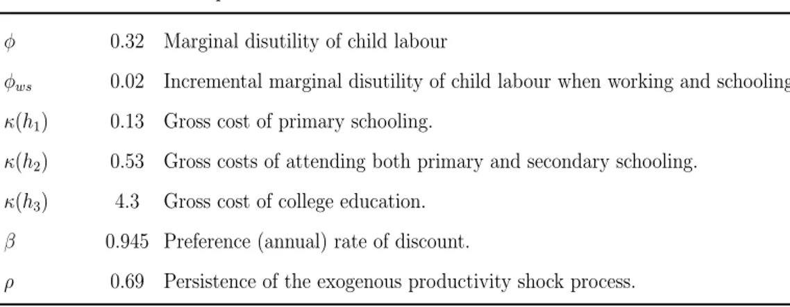
This section describes how we choose the model parameters, which include
A, a, γ, β, α, δ, ξ(·), κ(·),σ2, ρ,S(·), φ, φ
ws, andh.
Some parameters have a direct empirical counterpart. First, we normalize
A= 1. We also set the annual rate of depreciation to 0.06, so thatδ = 0.6507, as standard in the business cycles literature, and the borrowing constraint to a= 0.
In the first period, the time required to attend schooling is chosen as following. First, we suppose that schooling takes half of the child non-sleeping daytime. Moreover, we assume that, according with Brazilian legislation at the time17, the minimum number of school days is 200. Dividing this number
by the number of non-weekend days means that a child must attend schooling during roughly 75% of an year’s week days18.
In Brazil, secondary schooling requires three years while primary required eight at 199719. We assume, in this model, that every child completes at least
the fourth grade of primary school. Hence, in order to complete primary schooling, a child spends 12 · 34 · 174 = 8.8% of a period’s time endowment. Remember that the child’s effective endowment of time in the first period
17
Law 9394/96.
18
The same legislation states that these days should incorporate at least800 hours of
classes, excluding examinations. Since, in the time required to attend schooling, we also incorporate the other transaction costs such as transportation and exams time, we found it reasonable to assume that schooling requires 50% of a child non-sleeping hours.
19
is only 177. The same way, attending primary plus secondary school takes
1 2 ·
3 4 ·
7
17 = 15.5% of a period’s time.
We assume that college and working are mutually exclusive and that attending college requires 4.5 years20. Hence, the young adult who chooses
to go to college works for the remaining period time, which amount to 12.5 17 =
73.5% of a period time endowment.
7.1
The Wage Efficiency Profile
Our data source for estimation of ξ(t, h), the labour efficiency profile, is the
Pesquisa Nacional por Amostra de Domic´ılios of 1997. In order to calculate
the age efficiency profile, we restrict the data for the people who work 40-48 hours per week.
First, in order to obtain the values ofξ(1, h′), we need to take in account the dynasty’s decision for the child’s education. For example, if a child only goes to primary schooling and if he works the remaining time, at the end of the period he will have worked four years part-time with no investment in human capital and more three years full time, with the level of human capital being h1.
With this fact in mind, our hypothesis is that the (potentially) working child divides his labour hours proportionately to his available time in each condition. In the example above, hence, the child’s labour efficiency corre-sponds to an weighted average of four years working part time plus three years working full time, no matter how much of the available time is de-voted to working. Finally, we normalize ξ(2, h0) = 1, obtaining from the
data the average relative productivities ξ(1, h0) = 0.37, ξ(1, h1) = 0.48 and
ξ(1, h2) = 0.46.
20
In the baseline model, we restrict ξ(2, h) = ξ(3, h) for each h and also
ξ(4, h) = aξ(3, h), where ais obtained dividing the average wages of individ-uals who are 52-68 by the average wages of individindivid-uals from 18 to 51 years old. We then obtaina= 1.11. The relative wage premia, obtained using data for individuals from 18 to 68 years old, are set to ξ(2, h1) = ξ(3, h1) = 1.5,
ξ(2, h2) = ξ(3, h2) = 2.5, and ξ(2, h3) = ξ(3, h3) = 6.3.
7.2
Fiscal Policy
In Brazil, schooling is heavily subsidized, at all levels. For instance, in 2000, public expenditures on education, including federal, state and munic-ipalities, accounted for 3.9% of GDP21. In order to estimate the fraction
of public expenditures in education per student, we use information from two databases: The National Institute for Educational Research and Policy (INEP) and the Brazilian household expenditures survey22.
First, the INEP provides an estimate for public expenditures as a frac-tion of per capita GDP. We use the estimates for 2002, in order to match our data from POF. In 2002,for each student ranging from the fifth to the eighth level of primary schooling (10-14 years old), the expenditures per students accounted for 12.3% of the per capita GDP. The same ratio for secondary students was 8.9%, while for tertiary students it was 121%.
Given these ratios, we try to estimate the private expenditures in educa-tion per student. We use the 2002-2003 POF. For each family in this survey, we have information on expenditures in education, divided in six categories: (i) expenses in regular courses (any schooling up to secondary), (ii) expenses in tertiary courses23, (iii) total expenses in other courses, (iv) total
expen-ditures in books and scientific publications, (v) total expenexpen-ditures in school
21
Source: INEP/MEC
22
Pesquisa do Or¸camento Familiar, POF
23
articles, and (vi) others.
We then separate the families that spend only either on superior courses or regular courses. Therefore, we assume that a family that spends only on one of the categories devotes all other education expenditures in activities or goods linked to that category, which, in our model, are also considered expenditures in education. Finally, to assess the average expenditure per stu-dent, we suppose that every family has two heads and hence we divide the average expenditure for each category by the average household size minus two. Finally, since we do not have separate data for primary or secondary education, we suppose that the average private expenditures on both is the same.
Finally, we divide the obtained values by the 2002 per capita GDP. The result is that each tertiary education students privately costs 32.9% of the per capita income, while a student of a regular course costs on average 11.9%24.
We divide the government by the total expenditures to obtain the fraction of expenditures that the government subsidizes.
However, the way we define the subsidizing (S(·)) function requires a bit of modification of the previous obtained values. To start with, S(h2) equals
the value obtained with the method above, because every resource spent in secondary education is embedded in κ(h2). However, as the model states,
κ(h2) involves the cost of attending not only to secondary but also to
pri-mary school. So the true value of subsidy on pripri-mary schooling does not equal S(h1)25, but instead S(h1) is a function of the value obtained and the
quantity of children that attend each level of schooling.
We know that the (true) subsidy level equals s1,truegovernment expenditurestotal expenditures ,
24
The average family size for those who are enrolled in a superior course is 3.61, while for regular is 4.13. Samples sizes are respectively 4338 and 1555 observations.
25
for any given level of schooling. In our model, when it comes to the primary education, the true subsidy equals:
s1,true =
κ(h1)S(h1)d1+κ(h1)S(h2)d2
κ(h1)d1+κ(h1)d2
, (33)
where d1 = Pz,aλ1(z, h1, a) and d2 = P
z,a,hcλ2(z, h1, hc, a). By isolating
S(h1) in equation (33) we obtain the value of S(h1).
In sum, the value obtained is S(h1) = 46.5%. Moreover, we directly
obtain the other subsidy values from the data, which are S(h2) = 42.78%
and S(h3) = 78.63%26.
7.3
Exogenous Process for productivity
In order to approximate a continuous AR(1) process, we discretize it in the following way. First, in order to estimate the static variance of wages, we run the following regression:
log(wagei) = α+β1I[h=h1]+β2I[h=h2]+β3I[h=h3]+εi, εi ∼N(0, σ2) , (34)
from which we take the error variance and assume it is the unconditional variance of the exogenous AR(1) process (equation (3)) - our underlying hy-pothesis here is that the unconditional variance is the same regardless of the productivity level. To run the regression, we use data from PNAD for indi-viduals within the third period of the model, thus from 35 to 51 years old, normalizing the wagei relative to the average wage of an uneducated adult
from 35 to 51 years old.
Then, we use Tauchen’s method to discretize the AR(1). From the ob-tained data we can pin down σ, given a specific value of ρ27. Finally, ρ is jointly set along with κ(h1), κ(h2), κ(h3), φ, φws, and β, in order to match
26
The true value of the primary schooling subsidy is 50.79%.
27
The unconditional variance, σ2
several data features, which are explained below.
7.4
Targeted Moments
In sum, 27 parameters (some of which are part of the same functions) are taken from the literature or using hypotheses, given the data. The parameters are summarized in Tables 3 and 4. The remaining seven parameters are jointly chosen using the model to simulate a set of seven exactly identified empirical moments28. Let the parameter vector be:
Θ = [φws φ κ(h1)κ(h2)κ(h3)β ρ]′ (35)
The model generates seven moments, which we denote byM(Θ). The vector of empirical moments is denoted by Ms and summarized in Table 5. We find
the estimate for ˆΘ by:
ˆ
Θ = arg min
Θ {[M(Θ)]−Ms]
′W[M(Θ)−M
s]} (36)
where W is a weighting matrix. Here, we set W =I, since there’s no clear choice of W.
The calibration results are summarized in table 6.
7.5
Model Outcomes
In this section, I briefly introduce some outcomes related to poverty and inequality, which will be important in our future policy evaluation.
When it comes to wealth distribution, our model displays just one funda-mental source of heterogeneity, so it is expected that it will not generate the data income or wealth distribution (Cagetti and Nardi (2005)). However, de-spite its limitations on the issue, it performs reasonably well. The calibrated
28
model generates an income inequality, measured as the Gini coefficient on household per capita income (which, in our model, since all households have the same size, equals household income distribution), of 0.3965 - the true value for 1997, is instead 0.60 (according to the IPEA, who uses data from PNAD). On the other hand, the model’s wealth Gini equals 0.6502, while the estimated value in 2000 was 0.78.
We are also able to identify the poverty headcount ratio line, defined as the proportion of the population who earns less than two dollars (PPP 2005) a day, or 730 dollars a year. According to the world bank, 20.5% of the Brazilian population at 1997 earned less than two dollars a day. Using data for Brazilian PPP GDP, we see that the poverty line annual income represents 9.23% of per capita GDP29. In our policy experiments, we fix the
poverty headcount at the income level of the first 20.5 percentile of the pop-ulation in the baseline specification.
8
Introducing the Bolsa Fam´ılia
In this section, we introduce a conditional cash transfer and evaluate the new stationary equilibrium. We prefer not to face our results against existing literature (though they do point to the same direction) - we prefer, as pre-viously stated, to interpret our results as a potential long-term achievement of a continuous conditional cash transfer policy.
We set the transfer such that it represents 0.055% of the total income and is paid to 20.74% of the households, thus 41.5% of the households liv-ing through the first period, which fits true data in 2012. Notice that the proposed design benefits roughly the same share of the population as the share of households below the poverty line. Finally, transfers are only paid
29
to families who send their children to secondary school (so families who are living through their second period of the model do not receive the transfer). We also perform a counterfactual experiment, trying a different design. We provide a progressive transfer scheme, using the same income threshold as before. The families whose income are below half of the threshold earn a transfer 70% higher than the transfer paid in the previous experiment (hence-forth baseline CCT), while the families whose earnings lie between half the threshold and the threshold itself are given only 85% of the previous transfer. All in all, in the steady state equilibrium, the transfers account for the same share of the GDP and cover 17.1% of the population.
In the counterfactual experiment, less than 2% of the population were given the higher transfer, while the vast majority of the covered households, 16.5% of the total population, only received the smaller transfer. However, as we shall see, the cash transfer effects are reasonably stronger than in the baseline CCT, which suggests that progressiveness is a very important fea-ture of such a program.
It is also worth noticing the share of the population that chose not to get the transfer - in the baseline CCT formulation, this share accounted for 11.7% of the population, while in the progressive specification the share is only 6.8%. This fact also stresses the importance of a progressive transfer schedule. As in our model, there is evidence of undercoverage and mistar-geting in the actual Bolsa Familia design30.
Finally, we can also notice that, if we take into account the no transfer specification’s steady state distribution, we see that, in the baseline CCT,
30
56.3% of the covered households had already decided to sent their children to secondary school, while the same ratio for the progressive scheme was 34.4%. While the transfer is not designed only to induce a higher education, a progressive schedule seems to be best choice when it comes to this specific output.
8.1
Long Term Macroeconomic Effects
The results for macroeconomic variables are shown it Table 7. First of all, we have to notice that the CCT serves as an insurance for the house-holds, weakening precautionary motives, especially for those households who are at risk of being borrowing constrained (Zilberman and Berriel (2012)). This fact will play a crucial role in the program’s outcomes. On the other hand, we should expect the program’s incentives to education to increase the marginal return on physical capital, and thus mitigate the insurance ef-fect. Hence physical capital accumulation output will be defined by these two counteracting forces.
In the baseline CCT, it turns out that absolute capital level increases by 15%, but, as expected, the investment rate remains roughly constant, as shown in table (7). The partial elimination of the risk was not able to completely counterbalance the strong rise in human capital efficiency units, which, by itself, was responsible to an increase of 11% on the marginal pro-ductivity of capital. Insurance and education effects combined raised the interest rate by 0.4 percentage points. Finally, as expected due to the de-creased marginal return on labour, the (base) wages had a 4% decrease.
On the other hand, the progressive specification displays surprisingly good macroeconomic outputs.. Both output, human capital (in efficiency units) and absolute capital are even higher than in the baseline CCT.
as designed in this paper, encourages schooling (unless the families choose not to take the transfer). By construction, at least 32% of the adults, in a steady state equilibrium, have attended at least secondary schooling. In fact, secondary schooling matriculation raised by 33 percentage points, and was greatly responsible for the sharp increase in education in the economy as a whole. On the other hand, the cash transfer program was not fully able to encourage tertiary schooling, which raised by only 0.54 percentage points (roughly a 10% increase).
On the other hand, the progressive program exhibited roughly no increase in tertiary school enrolment, but a sharper increase in secondary schooling, 13% higher than in the previous specification.
8.2
Long Term effects on Child Labour
In the long-term, there are several general equilibrium effects that appear to be driving children out of the labour market, namely (i) children could re-duce labour supply to be eligible for the program, (ii) rere-duced precautionary motives, (iii) reduced basic wages, (iv) increased taxation, (v) more demand for leisure, due to alleviated poverty, and (vi) school enrolment requisites, which consumes children’s time endowment. It turns out that (iv) is proba-bly not true, for tax rates are roughly the same, as we shall see in the next sections.
the conditional transfer do not drastically change their children’s allocation of time.
In the progressive specification, we also see that, on average, the income of the families whose children work have raised. The income rise is consistent with data presented in table 2. In the baseline CCT specification, we see no changes in the wealth and incomes of the households whose children work. We’ll take a closer look at reasons for that in the “Targeted Families” section, where we will stress the importance of a progressive cash transfer scheme.
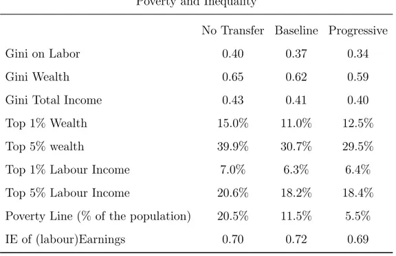
8.3
Long Term Effects on Poverty and Inequality
One of the main goals of the Bolsa Familia program is to reduce extreme poverty. Even the benefit scheme is designed with some degree of discre-tionary with regard to extremely poor families. To evaluate extreme poverty reduction, we consider the poverty line as being the income earn by the fam-ily in the first 20.5 percentile of the income distribution31. Also, in the period
between 1997 to 2012, income inequality in Brazil, measures as the Gini co-efficient, fell from 0.60 to 0.52. Despite our model’s limitations, it is possible to obtain useful insights on how the Bolsa Familia is able to reduce poverty. The results in this section are displayed in table 8.
The baseline specification has some impact on alleviating poverty - it re-duces the (total) income Gini coefficient by 1.7 percentage points, while the wealth Gini fell by 3.2 percentage points. We also see a slight reduction of the wealth and income share of the richest - for instance, the fraction of the labour income captured by the top 1 percentile falls from 7.04% to 6.33%. The reduction on the wealth share of the top 1 percentile is stronger, repre-senting 4 percentage points out of 15% in the no transfer specification.
31
On the other hand, the progressive cash transfer scheme is a powerful poverty-reduction policy. It outranks the baseline specification in every pre-sented aspect concerning poverty, except for the labour income share of the top percentiles. Despite this fact, since the progressive scheme is able to sharply reduce the Gini coefficient of labour income, we cannot say that it is not effective in reducing labour income inequality.
The channel through which both transfer schemes attack labour income inequality is clearly by bringing a large share of the population to secondary schooling, without significantly affecting tertiary school enrolment. Since the productivity shock is widely responsible for heterogeneity in this economy, we believe a 5.2 pp reduction in the Gini coefficient of labour income to be significant.
Nevertheless, the most impressive impacts of the conditional cash transfer programs come from reducing poverty directly, instead of reducing inequal-ity. The share of households who are below the poverty line (as defined in the section “Model Outcomes”) fall by 9.0 percentage points in the baseline CCT specification and by an astonishing 15.0 percentage points in the pro-gressive specification. Remember that all these results should be interpreted as a potential long-term poverty reducing power - so it is clear that it not the transfer itself that is able to bring households out of poverty, but, instead, the key here is the incentive to go to school.
intergen-erational elasticity of earnings32.
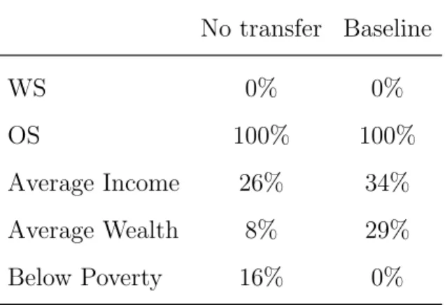
8.4
Targeted Families
In this section we evaluate how the targeted families reacted to the new policy. In the context of this model, the targeted families includes all the states x1 who receive the transfer. We evaluate those states before and after the introduction of the transfer, in their respective steady-state equilibria. The outcomes for the targeted families are listed in table 10.
The first fact here that jumps to one’s eyes is that the baseline CCT program is not able to reach the poorest. In fact, it does not reach families whose kids work, but only families whose kids were not planning to go to secondary school. Moreover, only 15.65% of the covered families are below the poverty line. However, at least in the sense of stimulating school regis-tration, the program is efficient. The fact that the transfer did not reach the poorest but the overall effects of the program were fairly beneficial gives a hint about the indirect power of such a policy.
In the baseline CCT program, the targeted households had their aver-age income increased by more than 26%, as well as a 8% increase in their wealth33.Also, the fraction of households below poverty in the targeted group
32
Soares et al. (2010) also report that the Bolsa Familia fails to affect the intergenera-tional persistence of earnings.
33
The way we compute these statistics are the following: we obtain the set of states that are eligible and choose to get the get the transfer. We then integrate the household income (which is a function of the state) over this set, both in the no transfer specification and in the baseline CCT specification. To conclude, what an increase in the average income of the targeted families tells us is that there was an increase on the relative measure (in the model, the function λ1(x1)) of those states with relatively higher income within the
falls almost to 0%34, which is particularly surprising if we take into
consid-eration that the transfer accounts for only 5.6% of the average income of targeted households. Hence, it is clear that the transfer plays an important role at the margin, taking many households who were previously “almost” indifferent between what level of education to choose to take their children to secondary school - in the long term, a virtuous circle is created, shifting the steady state equilibrium to one where there are more educated and wealthy families.
A more interesting and insightful case comes from the progressive cash transfer scheme, which is able to cover a larger part of the poorest families in the whole economy. We see that only by comparing the average income of the targeted families in this setup against the baseline CCT. Also, in this setup, there’s a group of families whose children are working and attending school both. This policy is not able to fully eliminate child labour in the targeted families - contrarily, it has a strong child labour reducing effect in the economy as a whole. Also, targeted families display a sharp increase in their wealth and income, and an almost total decrease in poverty - from 42.7
35 to less than 2% of the targeted families.
8.5
Welfare
Our last analysis concerns the welfare evaluations between steady state equilibria. To start with, let’s define the welfare, in consumption equivalent
34
The average income of those families whose children are not going to school but only working is below 40% the average income of the targeted families. Those families are in such a poverty situation that they choose not to accept the transfer.
35
units, for a given state, as being:
W1(x1) =
1 1−β
gc 1(1−γ)
1−γ
−(φ+I[h′ > h0]φws)gm1
, (37)
for the first period and:
W2(x2) =
1 1−β
gc 2(1−γ)
1−γ
, (38)
for the second period. To obtain the total economy’s welfare we just integrate over the possible states, using the invariant measure before the introduction of the new policy.
We only execute comparisons of steady state equilibria in our welfare analysis. Thus, contrary to what Zilberman and Berriel (2012) does, we do not claim anything about political support, neither we perform definite welfare analysis, since we do not compute the transition path in this model. Nevertheless, the steady state comparison is, if anything, suggestive.
To measure the equivalent variation of welfare in terms of consumption, we solve the following implicit equations for ∆:
(
(gc1+ ∆)(1−γ) 1−γ
!
−(φ+I[h′ > h0]φws)g1m
)
bef ore
=
(
(gc 1)
(1−γ)
1−γ
!
−(φ+I[h′ > h0]φws)g1m
)
af ter
,
(39)
in the first period and
"
(gc 2+ ∆)
(1−γ)
1−γ
!#
bef ore
=
"
(gc 2)
(1−γ)
1−γ
!#
af ter
, (40)
in the second period.
the targeted families than for the economy as a whole, in both specifications. Also the ratio of households that are better off after reaching the new equi-librium is impressive, especially in the progressive specification.
Finally, comparing the difference between steady-states in the total econ-omy’s welfare, we are able to answer the main question proposed by this paper. In the long-term, a conditional cash transfer as the Bolsa Familia, progressive or not, is able to substantially increase the economy’s total wel-fare.
9
Conclusion
In this paper, we evaluated the long-term quantitative effects of the Brazil-ian conditional cash transfer program, Bolsa Familia. We have proposed two transfer schedules: (i) transferring an equal amount to every family whose income is below a specific threshold, and (ii) providing a progressive transfer, with the lowest income families receiving a higher transfer. Both proposed policies are comparable, in the sense that the total amount of transfers as a ratio of the GDP (in the steady state equilibrium) are roughly the same, and the number of covered families is similar.
We find out that, no matter the schedule, the policy is able to significantly raise school registration and is fairly able to reduce child labour. The flat transfer scheme is able to raise the ratio of children who complete secondary school by 33 percentage points, lowering the ratio of children who do not attend school at all by 4 percentage points. It is also able to reduce the ratio working children from 22% to 15%. The transfer is also able to raise total output by almost 17%.
households, who prefer not to pay the secondary schooling costs and hence are not allowed the transfer.
All in all, the Bolsa Familia proves to be a strong policy instrument, not only benefiting the targeted families but also the households who aren’t el-igible. We believe that the most important aspect of such a policy is that it is almost does not distort the household optimal decisions - the increased taxation required to fund it is, in equilibrium, offset by the sharp increase in productivity and thus income - the result is that the tax rates can even
decrease in equilibrium. For instance, it is feasible that the raise in