Incentive-Driven Inattention
Ra¤aella
Giacomini
yWagner Piazza
Gaglianone
zJoão Victor
Issler
xVasiliki
Skreta
{November 10, 2015
Abstract
Keywords: Heterogeneity, Attention degree, Professional forecast-ers.
JEL Classification: E27, E37, D80, D83.
The views expressed in the paper are those of the authors and do not necessarily re‡ect those of the Banco Central do Brasil (BCB) or of Getulio Vargas Foundation (FGV). We are grateful to Valdemar Rodrigues de Pinho Neto for excellent research assistance and to the Investor Relations and Special Studies Department (Gerin) of the BCB for kindly providing the data used in this paper. Any remaining errors are ours.
yUCL. [email protected]
zResearch Department, Banco Central do Brasil. E-mail:
xGVF.
1
Introduction
Mankiw and Reis (2010) argue that the Phillips curve (or the aggregate
supply curve) is probably the most important macroeconomic relationship.
They state that “it is the key connection between real and nominal variables.
It explains why monetary policy, and aggregate demand more broadly, has
real e¤ects.” As is well known, the existence of a short-run trade-o¤ between
in‡ation and output gap relies heavily on some sort of inertia in price
expec-tations. Otherwise, as in Lucas (1972), although agents may not correctly
predict full-employment equilibrium at any point in time, their forecast
er-rors will still be unpredictable and the economy will ‡uctuate randomly about
full-employment – not a bad outcome.
The work of Mankiw and Reis (2002), Sims (2003) and Woodford (2003)
on inattention made the profession aware of the fact that the consensus
forecast among agents responded slowly to new information available to them;
see,inter alia, Coibion and Gorodnichenko (2012) and Andrade and Le Bihan
(2013). In some of these models inattention is assumed to be exogenous to
the agent, and in others it is assumed to be a function of the limited ability
of agents in processing information, while this limitation is itself exogenous
once we control for idiosyncratic random shocks. Of course, inattention can
generate a short-run trade-o¤ between in‡ation and output gap and have an
important role in the construction of the Phillips curve.
In this paper, we propose a novel approach in which we endogenize
inat-tention while retaining some important features of the previous literature.
In our framework, agents respond to incentives to update their predictions
based on new information, therefore the title Incentive-Driven Inattention.
New information ‡ows in continuously and acquiring information is costly.
To decide how much new information should be used in predicting future
in de…ning the bene…ts of updating information. We consider two di¤erent
regimes regarding incentives. In the …rst regime, incentives imply that agents
have high bene…ts for updating their forecasts, but in the second they have
no incentives and therefore are inattentive as in Mankiw and Reis, using
an exogenous updating rule. When they decide to update their information
set, they do not observe the true state, but receive noisy-information, as
in Sims and Coibion and Gorodnichenko (2014). Once we put together all
these ingredients, we have a structural macroeconomic model of
incentive-driven inattention, which can be tested at the individual level. Because we
can always aggregate individual data emulating a representative-agent
frame-work, we can also test previous results in the literature that were based on a
consensus-forecast approach.
To be able to evaluate and test the incentive-driven inattention model
we need to have access to high-frequency micro-data at the individual level,
where we can observe enough changes in costs and bene…ts of updating
in-formation. While most papers in the literature use consensus forecasts for
a representative agent, we are able to exploit the high-frequency micro-data
character of theFocus Survey gathered by the Brazilian Central Bank (BCB).
It has a few unique features that sets it apart from other well-known
expec-tation surveys. For example, its frequency of observations is daily
(work-ing days), as opposed to monthly (Wall Street Journal Forecasting Survey),
quarterly (Survey of Professional Forecasters), or semi-annually (Livingston
Survey). In our sample, dating from January 2nd, 2004 until January, 8th,
2015, at each working day, a survey respondent can choose to participate
inserting in the data base forecasts of a myriad of important macroeconomic
and …nancial forecasts for di¤erent horizons. An important feature of the
Focus-Survey design is that of incentives to participate at any given day,
which is related to reputation and accuracy of forecasts. The Focus
horizons are used to compute individual forecast errors and their
respec-tive mean-absolute-forecast-errors (MAFEs). Only forecasts at critical dates
are used to compute MAFE statistics at the individual level, and all
par-ticipants know this rule and when the critical dates are. Periodically, the
Central Bank compares MAFEs across individual institutions and releases
the names of the top …ve forecasting institutions for selected variables at
di¤erent horizons. Theoretically, since MAFE should not decrease with the
forecast horizon, institutions have an incentive to update forecasts at the
critical date to increase their chance of being listed as a top-…ve forecaster1.
In this paper, for mathematical convenience, and following the standard
ap-proach of the forecasting literature, we adopt as measure of forecast accuracy
the mean-squared-forecast-error (MSFE), which shares many properties with
the MAFE risk function, such as symmetry and strict monotonicity for
non-zero forecast errors.
The characterization, estimation, and testing of the incentive-driven
inat-tention model is done as follows. First, we document the di¤erence in
be-havior for critical and non-critical dates in forecasting in‡ation: a signi…cant
spike of updating forecasts in the data base – from about 12% on non-critical
dates to about 48% in critical dates. This spike coincides with a downward
structural break for the behavior of the consensus forecast MSFE across
dates. Second, we postulate a parsimonious cost-bene…t analysis model where
inattention di¤ers endogenously for critical and non-critical dates. Then,
af-ter Coibion and Gorodnichenko (2012), we compute the new updating rule
for the consensus forecast. To characterize the daily consensus forecast error,
1An informal incentive for respondents regards their invitation (inclusion) in a quarterly
we have to overcome the problem that it is a function of the daily
rational-expectation forecast error, while in‡ation is sampled at the monthly
fre-quency. Following Amemiya and Wu (1972), we use the fact that the best
representation for monthly in‡ation – an ARM A(1;1) model – corresponds
to anAR(1)model for daily in‡ation. Coupled with the interpolation method
used in Mönch and Uhlig (2005), we back out daily in‡ation and the daily
rational-expectation error in forecasting in‡ation. Third, as in Sims (2003),
and Coibion and Gorodnichenko (2014), we assume that agents never observe
the true state, but instead a noisy signal. This yields three structural
equa-tions to be estimated by Hansen’s (1982) generalized method of moments
(GMM) using daily data: the incentive-driven participation equation, the
AR(1) characterization for daily in‡ation, and the MSFE updating rule for
the consensus forecast. The model has six structural parameters: the two
participation parameters – critical and non-critical dates, the three AR(1)
parameters – constant, AR(1) coe¢cient and the variance of the error term
– and the variance of the noise in the signal-extraction problem.
Misspeci…-cation testing is done via the usual over-identifying-restriction J test.
When we take the model to the data, we obtain sensible structural
para-meters that are able to explain the dynamic behavior of the consensus MSFE
across dates, including the critical date. In misspeci…cation tests, the
struc-tural model is not rejected using a variety of instruments in GMM estimation.
Simulating the model also generates an MSFE pro…le that matches that of
the data when we consider a point-wise 95% con…dence interval around it.
We also investigate the determinants of updating information using a panel of
individual institutions. Our results show that updating is explained mostly
by the dummy variable of the critical date, followed by economic
uncer-tainty, measured by the Emerging Market Bond Index (EMBI).
Calendar-e¤ect dummies are also relevant, as well a the uncertainty of the individual
Equipped with our proposed model, we then discuss two important issues
in forecasting. First, using individual and consensus data, we perform a set of
rationality tests to investigate whether individuals or the consensus forecast
pass the rationality tests pioneered by Mincer and Zarnowitz (1969) and its
extensions in Coibion and Gorodnichenko (2014). Second, we discuss
survey-design issues, performing counter-factual exercises with our model in order to
assess the e¤ects of changing the incentive structure of the survey – a relevant
issue – since we believe that the expectation surveys of the future will have
the high-frequency structure of the Focus Survey, coupled with incentives
to update information, i.e., they will be similar to today’s Focus Survey on
those grounds.
When we apply a set of rationality tests to individuals or the consensus
forecast, results show that, at the individual level, at least 90% of individuals
are rational when we consider critical dates alone when they have proper
incentives to update forecasts. In contrast, for all dates, including non-critical
dates, at most 26% of individuals pass rationality tests. Similar tests applied
to panel-data and the consensus forecast show that rejection of rationality is
the rule, not the exception.
In our survey-design investigation, we show how one can choose the
Crit-ical Date in order to minimize the MSFE of the consensus forecast. We
perform two di¤erent counter-factual exercises. In the …rst, we ask what is
the best critical date within a standard month from the point of view of
a user of the consensus forecast. In the Focus Survey, the critical date is
currently in the mid-point of the working month – between two consecutive
releases of in‡ation data.2 However, to minimize the MSFE pro…le, the best
critical date is the day after the release of in‡ation data, since the updating
behavior in the model will lower the MSFE pro…le for the whole month. In
the second exercise, we compute what would be the gain of making every
day a critical day, starting just after the release of in‡ation, all the way to
the k-th working day within each month. Results show that the minimum
average MSFE is the one which every day is a critical date, which reinforces
the importance of proper incentives embedded in the critical date.
This paper is organized as follows. The next section discusses the Focus
data base and the stylized facts about updating behavior and the resulting
MSFE across dates. In Section 3 we present the details of the
incentive-driven inattention model proposed here. In Section 4 we present the empirical
evidence regarding the model – characterization, estimation, and testing. In
Section 5 we present the results of rationality tests and of the survey-design
counter-factual exercises for critical dates. In Section 6 we conclude.
2
The Focus Survey and Stylized Facts for
Updating Forecasts
2.1
The Focus Survey of the Brazilian Central Bank
(BCB)
The Focus Survey of expectations of the Central Bank of Brazil (BCB) is
unique in which it collects high-frequency data (working days) on 254
in-dividual institutions – about 100 of those are active at any point in time –
since 1999, although the number of participants increased substantially in the
mid 2000’s. Data collection started with the implementation of the
Brazil-ian In‡ation-Targeting Regime. Institutions include commercial banks,
as-set management …rms, consulting …rms, non-…nancial institutions and other
…rms with an assigned economist responsible for the information to be passed
on to the BCB. Forecasts are supplied over di¤erent forecast horizons and
indices, interest and exchange rates, GDP, industrial production, balance of
payments accounts, …scal variables, etc.
Our focus is on Brazilian in‡ation, measured by the Brazilian Consumer
Price Index – IPCA, the o¢cial target in‡ation monitored by the Brazilian
In‡ation-Targeting Regime. Our sample covers daily in‡ation forecasts
col-lected from January 2nd, 2004 until January, 8th, 2015 (2,751 workdays)3. In
each day t,t = 1; :::; T, survey respondenti, i= 1; :::; N, may inform her/his
expectations regarding in‡ation rates (or other variables) all the way up to
the next 18 months, as well as for the next 5 years on a year-end basis. For
example, market respondent i may inform on February, 2nd, 2004 her/his
forecast for the in‡ation rate of January, 2004 (not yet released), as well as
for February, 2004, and the following 16 months. Next working day, the same
agent may (or may not) update the forecasts for the same in‡ation rates of
January, 2004, February, 2004,..., up to June, 2005. This way, our sample
covers forecasts for the IPCA in‡ation from January, 2004 to December, 2014
(i.e. 132 months or events). The dataset forms an unbalanced panel (N T)
containing an amount of 234;605 observations. Decomposing our total
num-ber of observations into N and T, gives the following breakdown: T = 2;751
daily observations (only nowcasts), and an average of N = 85:3 forecasters
in our sample.
Besides its large size, the survey has other desirable features: (i) the
system access can be done at any time by survey participants, with no
pre-set schedule for updates; (ii) the con…dentiality of information is guaranteed
and the anonymity of forecasters is preserved (i.e., there are no reputation
concerns); (iii) the Focus Survey has speci…c incentives for participants to
update their forecasts (participate). The survey has periodical critical dates
in which forecasts for di¤erent horizons are used to compute individual
fore-3Since the survey had a small cross-sectional coverage (small N) in the beginning of
cast errors and their respective mean-absolute-forecast-error (MAFE). For a
given horizon, only forecasts at critical dates are used to compute individual
MAFE statistics and all participants know when critical dates are. The
Cen-tral Bank compares MAFEs across institutions and releases the names of the
top …ve forecasting institutions (individuals) for selected variables at
di¤er-ent horizons. This serves as an incdi¤er-entive scheme for survey responddi¤er-ents to
update their forecasts for the critical date; see Carvalho and Minella (2012)
and Marques (2013) for further details on the Focus Survey4.
Given its high-frequency character – daily observations – and the incentive
mechanism to update, the Focus Survey is well suited to investigate the issue
of incentive-driven inattention, since we have days in which participants have
an incentive to update their forecast and others where the opposite occurs. At
lower frequencies, it is hard to think about a similar incentive scheme being
operational, since, for example, it makes little sense to have a critical month,
quarter, or semester, respectively for the Wall Street Journal Forecasting
Survey, the Survey of Professional Forecasters, or the Livingston Survey.
Perhaps, for these low-frequency surveys, every observation is acritical date,
since the cost of updating once a month, a quarter, and a semester is low
relative to that of updating daily.
2.2
Stylized Facts
Critical Dates, Updating, and Accuracy
For the nowcast of monthly in‡ation, the chronology of relevant events is the
following: (i) IPCA in‡ation is usually released on the 8th of the month
sub-sequent to the reference month; (ii) on the 22nd of the reference month there
4The Focus survey is widely used in the Brazilian economy and its excellence has
is the release of IPCA-15 in‡ation, which contains important information
about IPCA in‡ation to be released in about 15 days; (iii) for every
refer-ence month, the critical date usually happens one day prior to the release
of IPCA-15 in‡ation. Thus, 17 days prior to the release of IPCA in‡ation.
Therefore, the critical date happens near the mid point between two
consec-utive monthly IPCA in‡ation releases.
In‡ation is only observed monthly, so choosing a critical day to compute
forecast errors and MSFE still gives one forecast error for every (monthly)
in‡ation observation. It also leaves a group of other days in which the
fore-caster has no incentive to update her/his forecast. So, this scheme introduces
variation across days in the micro data, which we can exploit to study
inatten-tiveness. Because the individual MSFE decreases with the forecast horizon
as a result of the use of more current information, and individuals want to
be among the group of top-…ve forecasters, theory implies that they should
update on the critical date, for which we should observe a spike in
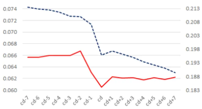
updat-ing. This is exactly what we observe in Figure 1, where the percentage of
individuals updating is displayed on the right scale. Although there is some
asymmetry for updating behavior on dates prior and after the critical date,
up to a reasonable approximation, the updating behavior is almost constant
around 12%, on average, but we observe a spike on the critical date of about
48% of individuals updating their information.
In Figure 1, when we also plot the MSFE of the consensus forecast for
current-month in‡ation (nowcast). We observe the usual (almost linear)
decline as the forecast horizon shrinks to zero. This is the result of the
acquisition of more and more information as time goes by and we approach
the in‡ation release date. However, for the MSFEs at the critical date and
later, we also observe a visible structural break: they are laying below the
position they should have been – the projection of the previous almost linear
The stylized fact we want to explain is essentially contained in Figure 1.
We want to have a model that links the increase in updating behavior due to
incentives with the structural break observed in the MSFE statistic for the
consensus forecast. We will endogenize updating behavior and link it to the
presence of incentives to update. At the same time, this massive movement in
updating behavior that we observe will have a downward e¤ect on the MSFE
statistic for the consensus forecast (an increase in accuracy), reducing it in
excess of what we would have observed in the absence of these incentives.
The model will be parsimonious and we will only distinguish between the
critical date and the non-critical dates, although there is some asymmetry
prior to and after the critical date that could still be modeled.
Figure 1 - Daily M SF E and ratio of updaters around the critical date (cd)
Critical Dates and Disagreement
Figure 2 shows the evolution of the disagreement around the critical date
based on two empirical measures: (i) Disagreement 1, which is the
cross-sectional standard deviation of individual forecasts – a measure of absolute
dispersion; and (ii) Disagreement 2, which is the standard deviation divided
by mean – a measure of relative dispersion.5 Both display a change in
behav-5In order to avoid computing a relative dispersion based on a mean forecast very close
ior in the critical date, where we observe a big drop in disagreement, some
of which is partially reverted in the next working day.
Overall, we observe a change in behavior either in MSFEs and in
Dis-agreement around the critical date. Given the obvious incentive mechanism
to update forecasts in it, we now turn into a model that accounts for
incentive-driven inattention.
Figure 2 - Disagreement around the critical date (cd)
Notes: Disagreement 1 is the cross-section standard deviation of individual forecasts, whereas Disagreement 2 is the cross-section standard deviation divided by the cross-section mean forecast.
3
The
Incentive-Driven Inattention
Model
We consider a model of the forecaster’s decision problem that is able to
replicate the stylized facts discussed above. The model builds on Mankiw
and Reis (2002), Sims (2003), Coibion and Gorodnichenko (2012, 2014), and
Andrade and Le Bihan (2013). It provides an endogenous mechanism that
can explain the observed variation in attention in our data base. The model
is the …rst to link inattention to the decision problem of the forecaster and
to investigate the forecaster’s incentives to provide a forecast in a context of
inattention.
The decision problem of an individual forecaster can be described as
fol-lows. At each day t, during a given month m, a forecaster i has the option
of logging into the BCB system to provide a forecast for the current month’s
in‡ation level ym, a nowcast problem. Let tCD represent the critical date
and consider a window of days before and after the critical date. At each
day t the forecaster decides to update the forecast if the bene…ts of doing
so outweigh the costs. The costs of updating could be due to a variety of
reasons, for example, obtaining information, processing information, running
a forecasting model, logging into the BCB system, etc. The bene…ts are due
to the higher chance of being in the group of top …ve forecasters – a clear
distinction among peers. This has a higher probability to occur if the forecast
in the BCB system is currently updated at t=tCD, since the more updated
a forecast is, the lower should be its M SF E.
We model the bene…t-cost ratio for each person at each point in time Bit
Cit, where Bit denotes bene…ts and Cit denotes costs, as a draw from a
Normal distribution with mean t and unit variance, so that the proportion
of forecasters who update at date t is given by:
t=P
Bit
Cit
>1 =P Bit
Cit t
>1 t = 1 (1 t); (1)
where ( )is the Standard Normal CDF.
Consider a model in which agents forecast monthly in‡ation, de…ned as
ym = logPm logPm 1 where Pm is the price level at the end of month
m: If yt = logPt logPt 1 is daily in‡ation, we must have ym = P21t=1yt;
where we have assumed for simplicity that there are 21 working days in a
standard month.6 At each date ta fraction
tof agents update their forecast
of monthly in‡ation ym. Here, we will need to account for both ym and yt,
since in‡ation is sampled every monthm, but the frequency of the data base
6In the empirical exercise we do take into account the fact that each month in our
is daily – t.
The incentive structure of theFocus Survey and the stylized facts shown
in Figure 1 above are consistent with the assumption that the distribution
of the bene…t-cost ratio across agents is constant over time, but has a mean
shift at the critical date due to the fact that the bene…ts of updating increase
dramatically for every forecaster at the critical date. At t = tCD, their
accuracy is recorded in order to form the ranking of the top …ve forecasters.
This setup implies that the mean of the bene…t-cost distribution evolves as:
t= 1 + 21 t=tCD ;
where 1 t=tCD is an indicator function of the critical date. This, in turn,
using (1), corresponds to a fraction of updaters that evolves as:
t= 1+ 21 t=tCD : (2)
To derive the properties of the consensus forecast implied by the model,
we build on Coibion and Gorodnichenko (2012) and adapt their result to
our setting of monthly in‡ation nowcasting with a time-varying proportion
of daily updaters. Coibion and Gorodnichenko show that, in models with
inattentive agents, the consensus forecast at time t; Ft; can be written as a
convex combination of the consensus forecast at the previous period, Ft 1,
and the current rational expectation of in‡ation, Et(ym):
Ft= tEt(ym) + (1 t)Ft 1; (3)
which implies that the consensus forecast error at time t is
ym Ft =
1 t
t
where vt=ym Et[ym]is a rational expectation error.
We now derive the implications of this result for the accuracy of the
consensus forecast in our setting. Here, the MSFE of the consensus forecast
at time t evolves as:
M SF Et=E (ym Ft)2 =
1 t
t 2
E ( Ft)2 +E v2t ; (5)
where we have used the fact that, by construction, vt is uncorrelated with
information available at time t.
To characterizevt=ym Et[ym], and compute the last term in (5) –E(v2t)
– we need a model for Et[ym]in a daily basis. The main problem here is that
we do not observe daily in‡ation, since it is sampled monthly. However, this
is simply an interpolation problem, which has been dealt with previously by
several authors, e.g., Mönch and Uhlig (2005), inter alia, in a multivariate
setting. In the simpler context of ARM A models, Amemiya and Wu (1972)
have general results for these processes, which we can apply to our case.
Their results show that, if the daily process is an AR(1), then, the monthly
process should be an ARM A(1;1), in a one-to-one mapping. Jumping to
our empirical section, this is exactly the process that best describes monthly
in‡ation, therefore we assume that daily in‡ation follows an AR(1) process:
yt= yt 1 +"t; "t i:i:d:N(0; 2"); (6)
which implies that the rational expectation of monthly in‡ation at day t is:
Et[ym] =Et
" 21 X
j=1
yj
#
= 21
X
j=t+1 j ty
which corresponds to a rational expectation error:
vt = ym Et[ym] = 21
X
j=1
yj 21
X
j=t+1 j t
yt
= "21+ (1 + )"20+:::+ (1 + +:::+ 21 t 1)"t+1;
and its variance is:
E v2t = 1 + (1 + )2+:::+ (1 + +:::+ 21
t 1)2 2
": (8)
The ARM A(1;1)process for monthly in‡ation ym as follows:
1 kL ym = (1 + L)"t;
where, in our case k = 21, since we assume that there are 21 working days
in a standard month. In the empirical implementation we will impose the
proper monthly restriction to each month, but for exposition purposes we
keep k = 21 here. Because ym =
P21
t=1yt, we are able to write a relationship
between "t and "t that will depend on and :
(1 + L)"t = 1 + L+:::+
k 1Lk 1 1 +L+:::+Lk 1 " t
= "t
"
kP1
i=0
Li
i
P
j=0 j
!
+ 2(kP1)
i=k
Li
2(kP1) i
j=0
k 1 j
!# :
Given consistent estimates for and , we can solve for 2
the following equations:7
(1 + 2) 2" = 2"
2 4kP1
i=0 i P j=0 j !2 +
2(kP1)
i=k
2(kP1) i
j=0
k 1 j
!23
5;or, (9)
2
" = 2"
"
kP1
i=1 i P j=0 j !
iP1
j=0 j
!!#
+ 2"
"
kP1
j=0 j
!
kP1
j=1 j !# + 2 " "
2(kP1)
i=k+1
2(kP1) i
j=0
k 1 j
!
2(k P1) i 1
j=0
k 1 j
!!# :(10)
We now introduce into the model a “lower bound” for MSFE by
employ-ing the “noisy-information” approach, where agents never fully observe the
true state, but instead receive a noisy signal as in Sims (2003) and Coibion
and Gorodnichenko (2014). First, recall that the monthly (observed)
in‡a-tion ym is modeled as the sum of the daily (latent) in‡ation yt, such that
ym =P21j=1yj. Each survey participant i does not observe the (latent) daily
in‡ationyt, but, instead, an idiosyncratic signalyi;t, such that yi;t =yt+ i;t,
where i;t i:i:d:(0; 2;i). If, as before, daily in‡ation follows an AR(1)
model, note that Ei;t(yi;t+h) = Ei;t(yt+h), sinceEi;t( i;t+h) = 0 for all h 1,
where Ei;t( )denotes the conditional expectation operator of participanti at
time t. Since the observed monthly in‡ation is the sum of the latent daily
in‡ation, it also follows that the sum of the daily signalsyi;t must be equal to
ym. Thus, ym =
P21 j=1yj =
P21
j=1yi;j and, therefore, the following restriction
holds: P21j=1 i;j = 0.
Let t = 1
N
PN i=1
Pt
j=1 i;j be the cross-section average of accumulated
7I one wishes to rely solely on the estimate of , then the following set of equations
can be viewed as a system of two equations with two unknowns that can be solved for and 2
i;t. Thus, the individual conditional expectation of ym can be written as:
Ei;t(ym) = Ei;t 21 X j=1 yi;j ! =Ei;t 21 X j=1
yj + i;j
!
= t
X
j=1
yj + i;j + 21
X
j=t+1 j t
yt = t
X
j=1
yj+ 21
X
j=t+1 j t
yt+ t
X
j=1 i;j:
The cross-section average rational expectation of ym is, then, given by:
1
N
N
X
i=1
Ei;t(ym) = Et(ym) + t:
Therefore, equation (3) becomes:
Ft = t(Et(ym) + t) + (1 t)Ft 1; (11)
where t i:i:d:(0; 2). Note that if 2 = 0, then, we are back to the Coibion
and Gorodnichenko (2012) updating formula as a special case.
Equation (11) implies now that a percentage t of attentive survey
par-ticipants update their forecasts in a (not fully) rational way, but instead
including some noise, due to the uncertainty regarding latent daily
in‡a-tion. By assuming that tis uncorrelated with vt and((1 t)= t) Ft, the
aggregated forecast error is given by:
ym Ft= ((1 t)= t) Ft+ (vt t);
and the respective MSFE is given by:
M SF Et=E (ym Ft)2 =
1 t
t 2
E ( Ft)2 +E vt2 +E 2
t : (12)
As long as the forecast horizon decreases, from (8) it follows thatE(v2
approaches 2
". Thus, for very short forecast horizons, even if E[( Ft)2]
and 2
" are close to zero, there is now a “residual” MSFE (or lower bound
for the MSFE) due to E( 2
t) = 2, which is not time-dependent, applies to
the whole term structure of M SF Et, and might help reconciling the model
outcome with the empirical evidence from data, as discussed below.
4
Empirical Analysis
We …rst assess the plausibility of theAR(1) model for in‡ation by estimating
anARM A(1;1)model for monthly in‡ation and backing out the
correspond-ing parameters and 2
" for the daily model as discussed in the previous
section. Then, we employ a state-space approach to construct the series yt
for daily in‡ation. Next, we compute the empirical counterparts of 1, and
2, which, together with , 2" and yt, allow us to uncover the right hand
side of equation (12), which can then be confronted with the actual MSFEs
reported in Figure 1. Our structural model has two other structural
equa-tions: equation (2), describing the evolution of the fraction of updaters, and
equation (6), describing the evolution of daily in‡ation. Once we consider
the use of proper instruments, the structural model can be estimated and
tested using the generalized method of moments (GMM).
To the best of our knowledge, this paper is the …rst to address such issues
in terms of incentive-driven inattention. The cost-bene…t model proposed
here should be viewed as complementary to the rational inattention
litera-ture, since it brings to it new and relevant topics, including survey design
and the dynamics of participants’ behavior. The model outcomes might also
be useful for policymakers interested in better understanding the evolution
of market expectations, which could help in designing an optimal-incentive
Modeling Monthly In‡ation
y
mFigure 3 shows the observed monthly in‡ation rate ym and the respective
daily consensus nowcast Ft. Table 1 presents the Akaike’s information
crite-rion (AIC) and the Bayesian information critecrite-rion (BIC) for models of the
ARM A class estimated for monthly In‡ation measured by IPCA. In both
cases, theARM A(1;1)belongs to the set of the three best models, the other
competitors being the AR(1), the AR(2), and the ARM A(2;1) model.
Ta-ble 2 presents the estimatedARM A(1;1)parameters. We discard theAR(1)
alternative given that the M A(1) coe¢cient is signi…cant at the usual
lev-els, which could also be a problem for the AR(2) model, and discard the
ARM A(2;1) because the ARM A(1;1)shows no signs of misspeci…cation in
its error structure, whereas the ARM A(1;1)is a more parsimonious model.
Figure 3 - Monthly in‡ation rate (ym) and daily consensus forecast (Ft)
-.
25
0
.25
.5
.75
1
01jan2004 01jan2006 01jan2008 01jan2010 01jan2012 01jan2014 01jan2016
daily consensus forecast monthly inflation rate
Table 1 - Information Criteria
AIC BIC
AR(1) -65.84 -57.19 AR(2) -66.19 -54.66 AR(3) -64.24 -49.83 AR(4) -65.25 -47.96 MA(1) -59.07 -50.42 MA(2) -63.44 -51.91 MA(3) -64.91 -50.50 MA(4) -63.37 -46.07 ARMA(1,1) -66.16 -54.63 ARMA(2,1) -65.87 -51.45 ARMA(1,2) -64.17 -49.76 ARMA(2,2) -63.87 -46.57 ARIMA(1,1,1) -59.36 -47.86 ARIMA(2,1,2) -58.18 -40.93
Note: The best three models according to each information criterion are marked in blue.
Table 2 - Model for monthly in‡ation rate: IPCA (ym)
ARMA(1,1): 1 kL y
m = (1 + L)"t
ck b c2
"
0:4544
(0:1261) 0(0:1220):2249 0(0:0046):0333
Note: Sample: January 2004-December 2014 (132 observations). Robust standard errors in parentheses.
Based on the estimation of the ARM A(1;1) model for the monthly
in-‡ation, we compute the corresponding estimates b = 0:9631 and b2
" =
1:1268E 05 of the AR(1) model for daily in‡ation (considering that each
month has a …xed number of k= 21 workdays).8
Constructing a daily in‡ation series
In order to generate a daily time series of in‡ation, we interpolate the
monthly in‡ation based on the method employed by Mönch and Uhlig (2005),
8For forecasting purposes, if one considers a month with k= 31calendar days, then,
it follows that the corresponding estimates become b= 0:9749and c2
which implements the state-space approach of Bernanke, Gertler and
Wat-son (1997). They consider an interpolation (or rather,distribution) problem
with mixed frequencies. Their complete model applied to unobserved daily
in‡ation yt would be:
(1 L)yt=xt +ut; with ut = ut 1+"t; (13)
where yt is the daily in‡ation, xt is a vector of covariates (observables) and
ut is an AR(1) error term, and observed monthly in‡ation ym is the variable
being interpolated. They impose the restriction that the daily interpolated
series yt exactly add up to the monthly observed in‡ation series ym in the
following way:9
ym =
8 > < > :
k
P
t=1
yt; t=k;2k;3k; :::; T
0; otherwise.
(14)
Monthly in‡ation can only be observed on dayst =k;2k; :::; T, and will
be the sum of the corresponding daily in‡ation rates in any given month.
Otherwise, it is just set to a …ctional value of zero. Notice that setting
ym = 0for the days we do not observe it is a way of making monthly in‡ation
9Since the interpolation methodology requires the use of balanced data, we considered
observable at the daily frequency. The corresponding state-space model is:10
ym = H0t t, where, (15)
t = 0 B B B B B B B B B B B @ yt
yt 1
yt 2 ...
yt k
ut 1 C C C C C C C C C C C A 0 B B B B B B B B B B B @
0 0 : : : 0
1 0 0 0 0 0
0 1 0 0 0 0
..
. . ..
0 0 0 1 0 0
0 0 0 0 0
1 C C C C C C C C C C C A 0 B B B B B B B B B B B @
yt 1
yt 2
yt 3 .. .
yt k 1
ut 1
1 C C C C C C C C C C C A + 0 B B B B B B B B B B B @ xt 0 0 ... 0 0 1 C C C C C C C C C C C A + 0 B B B B B B B B B B B @ "t 0 0 .. . 0 "t 1 C C C C C C C C C C C A ; (16)
and (15) and (16) represent, respectively, the observation and state equations.
The matrix H0t is time-varying with the following format:
H0t=
8 < :
[1 1 1 : : : 1 0]; t=k;2k;3k; :::; T
[0 0 0 : : : 0 0]; otherwise. (17)
To apply Mönch and Uhlig’s setup to our problem ofinterpolating monthly
in‡ation, we set to 0:9631 (which is the estimate from the ARM A(1;1)
AR(1)approach of Amemiya and Wu, 1972) and set = = 0in the system
10In the Kalman-…lter literature for mixed frequency models (e.g., Giannone, Reichlin
(15), (16) and (17). This yields our corresponding daily AR(1) model:
yt = yt 1+"t;
with an embedded interpolating restriction, which is consistent with the
ARM A(1;1) model estimated with monthly data. Results are presented
in Figure 4.
Figure 4 - Daily in‡ation rate (yt) series based on
the state-space model with = 0:9631
-.
01
0
.01
.02
.03
01jan2004 01jan2006 01jan2008 01jan2010 01jan2012 01jan2014
GMM Estimation of the
Incentive-Driven Inattention
model
We propose the joint estimation the structural parameters of our model using
the generalized method of moments (GMM) based on three moment
condi-tions derived from the cost-bene…t model of incentive-driven inattention. The
…rst is the equation …tting the observed time-varying degree of attention t
using equation (2), with two structural parameters – 1 and 2. Since we
observe the proportion of agents updating in each point in time (days), we
have an empirical measure of t from the data, which we confront to our
model in equation (2). The second equation is the square of equation (6) for
daily in‡ation yt (including an intercept c), which was estimated using the
the evolution of the M SF Et using (12), where we can compute the daily
MSFE in nowcasting in‡ation from the data, which can then be confronted
with our model. The three structural equations are:
t 1 21t=tCD = 0;
(yt c yt 1)2 "2t = 0;
M SF Et
1 t
t 2
E ( Ft)2 E vt2 E 2t = 0: (18)
From (8), it follows that E(v2
t) = wt 2", where wt [1 + (1 + )2 +:::
+(1 + +:::+ 21 t 1)2]. Taking the conditional expectation E( j F
t 1) on
both sides of the three equations in (18), where Ft 1 is the information set
available at time t 1, and using respectively for each equation the set of
valid instrumentsz1;t 1,z2;t 1, andz3;t 1, the system (18) can be written as a
system of restrictions on the set of structural parameters 1; 2; c; ; 2"; 2 ,
as follows:
0 = E[( t 1 21t=tCD) z1;t 1]; (19)
0 = E (yt c yt 1)2 2" z2;t 1 ; (20)
0 = E
2 4
0
@ M SF Et
1 1 21t=tCD
1+ 21t=tCD
2
E[( Ft)2]
wt 2" 2
1
A z3;t 1
3 5; (21)
where the vector of instruments include an intercept and other observables
dated ont 1and older, anddim(zj;t 1) =nj 1; j =f1;2;3g. There are six
structural parameters 1; 2; c; ; 2"; 2 to be estimated and(n1+n2+n3)
moment conditions. Over-identi…cation requires that (n1+n2+n3)>6.
In GMM estimation, we are treating the following as observables: t,
M SF Etand1t=tCD. In addition, we also treated as observables the following
variables: yt, wt and Ft, where yt comes from the (Kalman-…ltered) daily
and wt [1 + (1 + )2+::: +(1 + +:::+ 21 t 1)2], and Ft is constructed
using the Coibion and Gorodnichenko (2012) updating formula, which, in
turn, relies on the observed series t and on the constructed series Et(ym),
generated fromytandb.11 We also did some robustness analysis regardingFt,
since we can get a daily observed consensus forecast from the Focus Survey.
Table 5 presents the GMM estimates12 from two di¤erent sets of
instru-ments.13 The over-identifying-restrictions (OIR) are tested using theJ test
due to Hansen (1982). The joint signi…cance of the variance terms 2
" and 2
is also veri…ed.
11In addition, as an initial value, for every month (or event), the …rst consensus forecast
from the Coibion and Gorodnichenko formula is set equal to the respective consensus forecast from data.
12The "iterative" procedure of Hansen et al. (1996) is employed in the GMM estimation
and the initial weight matrix is the identity.
13Set of instruments I: z
1;t 1 = [1; Ft 2; :::; Ft 4]0; z2;t 1 = [1; t 2; :::; t 5]0 and z3;t 1= [1; yt 2; :::; yt 5]0. Set of instruments II:z1;t 1= [1;
2
Ft 1; :::; 2
Ft 3]0; z2;t 1=
[1; t 1; :::; t 3]0 and z3;t 1 = [1; yt 1; :::; yt 3]0. This way, for the …rst set of
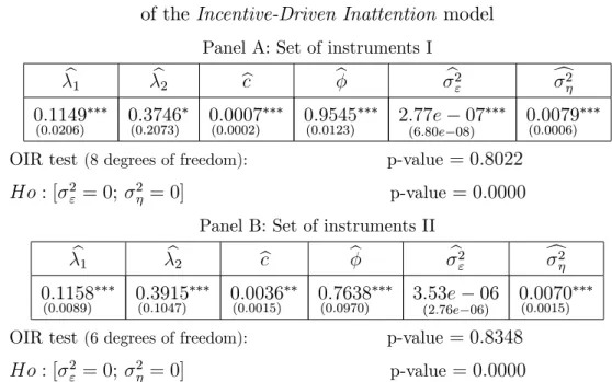
Table 5 - GMM estimates of the structural parameters
of theIncentive-Driven Inattention model
Panel A: Set of instruments I
b1 b2 bc b b2
" c2
0:1149
(0:0206) 0(0:2073):3746 0(0:0002):0007 0(0:0123):9545 2:(6:80e77e 08)07 0(0:0006):0079
OIR test(8 degrees of freedom): p-value = 0:8022
Ho: [ 2
" = 0; 2 = 0] p-value= 0:0000
Panel B: Set of instruments II
b1 b2 bc b b2
" c2
0:1158
(0:0089) 0(0:1047):3915 0(0:0015):0036 0(0:0970):7638 3:(2:76e53e 06)06 0(0:0015):0070
OIR test(6 degrees of freedom): p-value = 0:8348
Ho: [ 2" = 0; 2 = 0] p-value= 0:0000
Notes: (i) Robust Newey-West SE in parentheses. (ii) ***, **, * indicate signi…cance at 1%, 5% and 10% levels, respectively. (iii) OIR denotes the Over-Identifying Restriction J-test due to Hansen (1982).
(iv)Ftused here is constructed using the Coibion and Gorodnichenko (2012) updating formula. In both estimation setups, the over-identifying-restriction test is not
re-jected at the usual levels of signi…cance. The joint test for the zero variances
involving 2
" and 2 is rejected at any admissible level in both instances,
al-though the 2
" is not signi…cant in Panel B above. By comparing the point
estimates from the two sets of instruments, one should note that the
esti-mated parameters b1; b2 and c2 remained quite stable, although the point
estimatesbc; b and b2
", have changed.14
Next, we perform the estimation of the system in (19), (20), and (21),
14In this case, note that for a given time seriesy
t=c+ yt 1+"t; and its respective
unconditional meanE(yt) =c=(1 ), it follows that a decrease in the autoregressive
parameter (e.g., due to a change in the set of instruments in a GMM estimation) might lead to an increase in the variance of residuals 2
" and, at the same time, imply an
increase of the intercept c (provided that remains unchanged). This is exactly the observed change in point estimatesbc;b andc2
"when one goes from the GMM estimation
using observed Ft – the daily observed consensus forecast from the Focus
Survey – instead of that obtained using Coibion and Gorodnichenko’s (2012)
updating formula. Results are presented in Table 6.
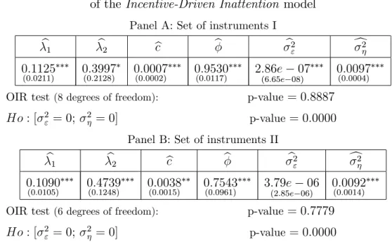
Table 6 - GMM estimates of the structural parameters
of theIncentive-Driven Inattention model
Panel A: Set of instruments I
b1 b2 bc b b2
" c2
0:1125
(0:0211) 0(0:2128):3997 0(0:0002):0007 0(0:0117):9530 2:(6:65e86e 08)07 0(0:0004):0097
OIR test(8 degrees of freedom): p-value = 0:8887
Ho: [ 2
" = 0; 2 = 0] p-value= 0:0000
Panel B: Set of instruments II
b1 b2 bc b b2
" c2
0:1090
(0:0105) 0(0:1248):4739 0(0:0015):0038 0(0:0961):7543 3:(2:85e79e 06)06 0(0:0014):0092
OIR test(6 degrees of freedom): p-value = 0:7779
Ho: [ 2
" = 0; 2 = 0] p-value= 0:0000
Notes: (i) Robust Newey-West SE in parentheses. (ii) ***, **, * indicate signi…cance at 1%, 5% and 10% levels, respectively. (iii) OIR denotes the Over-Identifying Restriction J-test due to Hansen (1982).
(iv)Ftused here is the daily observed Consensus Forecast from the Focus Survey.
The robustness exercise presented in Table 6 shows very similar results
to those in Table 5. All in all, we obtained sensible and mostly signi…cant
structural parameters that are able to explain the dynamic behavior of the
consensus MSFE across dates, including the critical date. In misspeci…cation
tests, the structural model is not rejected using a variety of instruments in
GMM estimation. We now turn to the motivating picture of this paper –
Fig-ure 1 – asking whether or not the estimated structural model can reproduce
the MSFE pro…le depicted there.
the one implied by theIncentive-Driven Inattentionmodel, when GMM point
estimates are used to construct the MSFE pro…le. We also include
OLS-estimated parameters for comparison; see the Appendix.
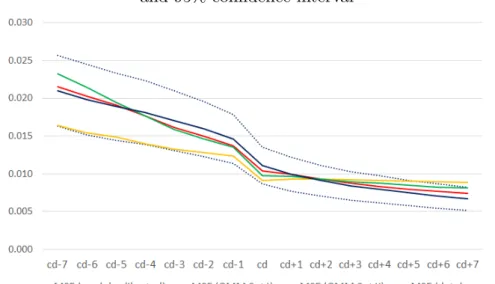
Figure 5 - MSFE (Data versus GMM-estimated and OLS-estimated)
and 95% con…dence interval
Note: Con…dence interval based on (pointwise) asymptotic values: std. error = sample std.dev.=pT, whereT = 132events (or months) for each investigated dateCD+j; j = 7; :::;7.
First, note that all threeM SF E curves implied by the model fall inside
the asymptotic 95% con…dence interval for the observed M SF E – a small
exception for GMM using set of instruments I, at cd+6 and cd+7. This
con-…rms the usefulness of the Incentive-Driven Inattention model in explaining
what we observe for the MSFE pro…le.
Second, note that the MSFE curve from the second set of instruments
(in the GMM setup) provides better results compared to the …rst set of
instruments. A possible explanation is the point estimate b2
", which is more
than ten times higher in the second set of instruments (compared to the …rst
Finally, note that all three curves implied by the model capture quite
well the sharp decrease in MSFE at the critical date (cd), which is due to
the fact that the point estimates for the attention parameters 1 and 2 are
similar across these three approaches (i.e., OLS-two-step, GMM set I, GMM
set II) and re‡ect reasonably well the observed series t through equation
t= 1+ 21t=tCD.
Modeling the Probability of Updating (Logit/Probit)
This section presents the estimates of an econometric model of the probability
of updating in a panel-data context. It is a reduced-form model for the
dependent variable i;t, the unobserved willingness to update information.
We do not observe i;t. However, we do observe i;t, which shows whether or
not agent i has updated information in periodt:
i;t =
8 < :
1 if i;t >0
0 if i;t 0.
The reduced form for i;t is the following:
i;t = i+xt +zi;t 1 +e2i;t +"i;t; (22)
where i is the unobserved heterogeneity, captured by either …xed or
ran-dom e¤ects; the x0
t = [dmont ;dtuet ;dthut ;d f ri
t ;dCDt ;d ipca
t ; d
ipca15
t ;dM P Ct 1 ]0 vector
contains the following variables: dmon
t ;dtuet ;dthut andd f ri
t are dummies for the
days of the week (workdays only), dCD
t is a dummy for the critical date,d
ipca t
and dipca15t are dummies for the days of release of the IPCA and IPCA15,
respectively, and dM P C
t 1 is a dummy for the (lagged) day of release of the
minutes of the meeting of the Monetary Policy Committee (MPC) of the
captured by the Emerging Market Bond Index (EMBI) for Brazil – the daily
risk premium on Brazilian sovereign debt; e2
i;t is is the squared forecast error
made by respondent i in the previous month. The parameters in , , and
are estimated using a panel Probit or Logit model,15 based on …xed e¤ect
(only Logit16) or random e¤ects (both Logit and Probit). This amounts to
choosing the parametric form of G( )in:
Pr i;t = 1 xt; zi;t 1; e2i;t =G i+xt +zi;t 1 +e2i;t ;
where G( ) can take the form of a conditional Normal CDF for the Probit
model or the conditional Logistic CDF for the Logit model.
In order to get comparable estimated coe¢cients, we standardized all
regressors (i.e., zero mean and unit variance, by demeaning and dividing
each regressor by its respective sample standard deviation). The estimation
results are presented below in Table 8:
15In order to estimate the referred panel models we assume strict exogeneity, in which
the explanatory variables in each time period are uncorrelated with the idiosyncratic er-ror in each time period; which is a much stronger assumption than simply assuming no contemporaneous correlation.
16Performing …xed e¤ects Probit estimation is more complicated than its Logit analog,
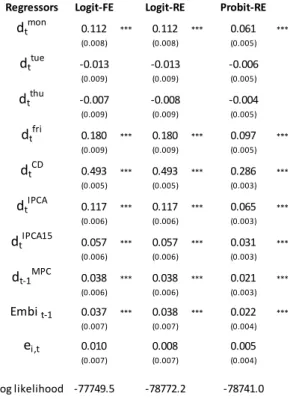
Table 8 - Panel Logit/Probit model of the probability of update
(dependent variable: i;t)
Regressors Logit-FE Logit-RE Probit-RE
dtmon 0.112 *** 0.112 *** 0.061 *** (0.008) (0.008) (0.005)
dttue -0.013 -0.013 -0.006
(0.009) (0.009) (0.005)
dt thu
-0.007 -0.008 -0.004
(0.009) (0.009) (0.005)
dtfri 0.180 *** 0.180 *** 0.097 *** (0.009) (0.009) (0.005)
dtCD 0.493 *** 0.493 *** 0.286 *** (0.005) (0.005) (0.003)
dt IPCA
0.117 *** 0.117 *** 0.065 *** (0.006) (0.006) (0.003)
dtIPCA15 0.057 *** 0.057 *** 0.031 *** (0.006) (0.006) (0.003)
dt-1MPC 0.038 *** 0.038 *** 0.021 *** (0.006) (0.006) (0.003)
Embit-1 0.037 *** 0.038 *** 0.022 *** (0.007) (0.007) (0.004)
ei,t 0.010 0.008 0.005
(0.007) (0.007) (0.004)
Log likelihood -77749.5 -78772.2 -78741.0
Notes: FE means …xed e¤ects and RE random e¤ects. Robust standard errors in parentheses. Number of observations = 223,685. *** indicates 1% signi…cance level.
The main result in Table 8 is that the dummy for the Critical Date –
dCD
t – is the most important variable in explaining the probability of agent
i updating her/his forecast in dayt. Given that we normalized all regressors
to have zero mean and unit variance, we can compare coe¢cients in the Logit
and Probit regressions. Note that, in absolute value, the estimated coe¢cient
of dCD
t is at least 2.5 times that of the second largest coe¢cient –d
f ri
t .
It is also worth noting that the impact of the IPCA release is higher
in comparison to that of the release of IPCA15 and of the Central-Bank
minutes. Moreover, the coe¢cient for the past squared forecast error is not
signi…cant, but the coe¢cient for uncertainty (EMBI) is positive and
coe¢cients for the calendar-e¤ect dummies.
With respect to the dummies for the weekdays, the highest estimated
co-e¢cient was for the Friday dummy. This can be related to a market readout
published on every Monday morning by the Central Bank of Brazil
(Focus-Market Readout). It releases key aggregate statistics from theFocus Survey,
such as the consensus forecast, the median, the standard deviation, the
coef-…cient of variation, the maximum and minimum, etc., based on data collected
up to 5 PM of the previous Friday. See Marques (2013, p. 305) for further
details.
Finally, note that the Logit coe¢cients obtained from …xed e¤ects are
very close to the ones from the random e¤ects model. In comparing the
coef-…cients estimated by the Probit and Logit models, Amemiya (1985) suggests
multiplying a Logit estimate by 0:625 to get an estimate of the
correspond-ing Probit estimate, since their respective distributions have zero mean, but
their variances are di¤erent (1 for the Normal and 2=3 for the logistic). In
this respect, our empirical results are matched in most cases.
5
Rationality Tests and Survey Design
In this section, we provide evidence that results of rationality tests are
severely a¤ected if one disregards the di¤erent behavior of agents in
crit-ical and non-critcrit-ical dates. Moreover, we also provide evidence that test
results based on a time-series of individual forecasts are very di¤erent from
those using the time-series of the aggregate measure of consensus forecasts
or panel-data on individuals under homogeneity restrictions.
When testing individuals separately, at the critical dates alone, we …nd
compelling evidence of rationality, whereas we …nd the opposite in di¤erent
contexts: non-critical dates, all dates, time-series of the consensus forecasts,
the importance of understanding and modellingincentive-driven inattention.
The latter is not merely a curiosity found in an exquisite data-base, but
something that must be understood as we gather more frequent time-series
observations in panels of forecasts. It also has a bearing on survey design,
where surveys are taken in high frequency (weekly, daily, or tic by tic) and we
consider changes in the incentive structure of the survey in order to reduce
the MSFE for the survey user. Since we believe that the expectation surveys
of the future will be of that kind, this paper provides a step forward in
designing their structure.
Rationality tests
Let t+h be the in‡ation rate as measured by the IPCA, fi;t+hjt be the
re-spective in‡ation forecast of survey participant i formed at period t, and
Ft+hjt be the consensus forecast, i.e., Ft+hjt = N1 PNi=1 fi;t+hjt. We
consid-ered six sampling schemes, due to the possibility of using aggregated or
disaggregated data in both dimensions. The time dimension can be
com-puted in two ways: daily frequency (T = 2;751 workdays), where we use
all days in the sample, or in monthly frequency (T = 132 months), where
we use only critical dates. The cross-section dimension can be considered
in three ways: (i) disaggregated data, with an individual OLS regression for
eachi= 1; : : : ; N17; (ii) disaggregated data, with panel data linear regression
(random-e¤ects or …xed-e¤ects models); and (iii) aggregated data (consensus
forecast), with OLS regression. On the other hand, we considered three types
of rationality tests: (1) Mincer-Zarnowitz (MZ) regressions; (2) FIRE
(Full-Information Rational Expectations) tests, from Coibion and Gorodnichenko
(2014, equation 10); and (3) FIRE tests, weaker version, from Coibion and
Gorodnichenko (2014, equation 12).
17In each test with disaggregated data (individual OLS regressions), we only considered
Mincer-Zarnowitz Tests
First we consider disaggregate data, with an individual OLS regression for
each i = 1;2; : : : ; N. The individual-forecasts OLS regressions are given as
follows:
t+h = i+ ifi;t+hjt+"i;t+h; (23)
where, t+h denotes observed in‡ation on period t+h, and fi;t+hjt denotes
individual i forecast of t+h using only information up to period t. The
Mincer and Zarnowitz (1969) test is based on a Wald test of the joint null
hypothesis of rationality, H0 : [ i = 0; i = 1] for each i. We then compute
the proportion of agents for which we do not reject the null of rationality.
Next, we consider disaggregate data in a panel-data linear-regression
(random-e¤ects or …xed-e¤ects models) context:
t+h = + fi;t+hjt+vi+"i;t+h; (24)
wherevi is the unobserved heterogeneity and"i;t+h is the error term, and, due
to the curse of dimensionality, we impose the homogeneity restriction that
i = for all i= 1;2; : : : ; N. Here, the Mincer-Zarnowitz test of rationality
is based on a Wald test of the joint null hypothesis H0 : [ = 0; = 1].
At last we consider aggregate data (consensus forecast), with OLS
re-gression in time-series data. The consensus-forecast OLS rere-gression is given
by:
t+h = + Ft+hjt+"t+h; (25)
where the rationality test is based on a Wald test of the joint null hypothesis
H0 : [ = 0; = 1]. In testing all the null hypotheses listed above we have
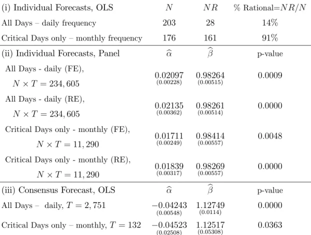
Table 9 - Mincer-Zarnowitz (MZ) regressions
(i) Individual Forecasts, OLS N N R % Rational=N R=N
All Days – daily frequency 203 28 14%
Critical Days only – monthly frequency 176 161 91%
(ii) Individual Forecasts, Panel b b p-value
All Days - daily (FE),
N T = 234;605 0(0:00228):02097 0(0:00515):98264 0:0009
All Days - daily (RE),
N T = 234;605 0(0:00362):02135 0(0:00514):98261 0:0000
Critical Days only - monthly (FE),
N T = 11;290 0(0:00249):01711 0(0:00557):98414 0:0048
Critical Days only - monthly (RE),
N T = 11;290 0(0:00317):01839 0(0:00557):98269 0:0000
(iii) Consensus Forecast, OLS b b p-value
All Days – daily, T = 2;751 0:04243
(0:00548) 1(0:0114):12749 0:0000
Critical Days only – monthly,T = 132 0:04523
(0:02508) 1(0:05308):12517 0:0363
Note: Robust standard error in parenthesis. FE means …xed-e¤ects and RE means random-e¤ects. In the second column,N indicates the number of survey participants with at least
10 observations. In the third column,N Rindicates the number of rational participants (p-value>0.05 in the rationality test).
Results in Table 9 show compelling evidence that incentives are
impor-tant to understand the results of rationality tests. First, when we consider
all the days in our sample, tests using Mincer-Zarnowitz regressions with
dis-aggregate data and individual OLS regressions for eachishow that only14%
of the individuals pass rationality tests at the 5% signi…cance level, i.e., for
only 14% of the individuals we cannot reject the null hypothesis. However,
com-pletely di¤erent in which we cannot reject the null of rationality for 91% of
the individuals at the 5% level. A natural conclusion is that incentives
mat-ter for rationality-test results. As argued above, in critical dates, individuals
become more attentive and this additional attentiveness reduces inertia in
in‡ation expectations, changing the results of rationality tests. For critical
dates, rational behavior is the rule, not the exception.
In Table 9, we also consider disaggregate data in a panel-data
linear-regression context, where we impose homogeneity restrictions ( i = ;8i) in
testing the joint null hypothesis H0 : [ = 0; = 1]. Here, in testing the
null, we have the auxiliary hypothesis of homogeneity. Hence, rejection can
also be due to homogeneity itself. Regardless of whether we consider critical
or non-critical dates, the null is always rejected at the 5% level, or even at
the 1% level.
Finally, we analyze test results using the consensus forecasts with OLS
regressions. The null is always rejected at the5%level, regardless of whether
we consider critical or non-critical dates, which is consistent with results
pre-viously found in the literature, where rationality was rejected overwhelmingly
in Mincer-Zarnowitz tests.
Next, we provide a summarizing picture of the results of rationality tests
using individual time-series data for non-critical and critical dates,
Figure 10 - P-values of the joint test Ho: [ i = 0; i = 1] for each i
Case (i) Individual Forecasts, OLS (daily frequency)
Notes: The p-value (vertical axis) of the rationality test based on the MZ regression is plotted by each survey participant (horizontal axis).
Figure 11 - P-values of the joint test H0 : [ i = 0; i = 1] for eachi
Case (i) Individual Forecasts, OLS (only critical dates, monthly freq.)
FIRE Tests
In this section we consider full-information rational-expectation (FIRE) tests
as used in Coibion and Gorodnichenko (2014, Equation 10). They are a
vari-ant of the Mincer-Zarnowitz tests. For individual forecasts, OLS regressions,
we run:
t+h fi;t+hjt = i+ i fi;t+hjt fi;t+hjt 1 + i;t+h; (26)
where the FIRE test is based on the null of rationality, H0 : [ i = i = 0]
for each i. We then compute the proportion of agents for which we do not
reject the null of rationality. For individual forecasts, panel-data regression,
we run:
t+h fi;t+hjt = + fi;t+hjt fi;t+hjt 1 +vi+ i;t+h; (27)
where vi is the unobserved heterogeneity, and the FIRE test is based on the
null H0 : [ = = 0]. For the consensus forecast, OLS regression, we run:
t+h Ft+hjt = + Ft+hjt Ft+hjt 1 + t+h; (28)
where the FIRE test is based on the null H0 : [ = = 0]. Results of FIRE
Table 10 - FIRE Test Results
(Full-Information Rational-Expectation Tests)
(i) Individual Forecasts, OLS N N R % Rational=N R=N
All Days – daily frequency 203 52 26%
Critical Days only – monthly frequency 171 157 92%
(ii) Individual Forecasts, Panel b b p-value
All Days - daily (FE),
N T = 233;120 (2:00E0:013257) (0:00635)0:10445 0:0000
All Days - daily (RE),
N T = 233;120 0(0:00271):01351 (0:00635)0:10447 0:0000
Critical Days only - monthly (FE),
N T = 10;710 (8:51E0:0095607) (0:00639)0:02925 0:0000
Critical Days only - monthly (RE),
N T = 10;710 0(0:00155):01058 (0:00640)0:02908 0:0000
(iii) Consensus Forecast, OLS b b p-value
All Days – daily, T = 2;750 0:01382
(0:00209) 0(0:11122):28923 0:0000
Critical Days only – monthly,T = 131 0:00987
(0:00905) 0(0:07264):14912 0:0411
Notes: Standard error in parenthesis. FE means …xed-e¤ects and RE means random-e¤ects. In the second column,N indicates the number of participants with at least 10 observations.
In the third column,N Rindicates the number of rational participants (p-value>0.05 in the rationality test). The lagged forecast is related to the previous day (in daily frequency)
and to the previous month (i.e., previous critical date, in the monthly frequency).
Results in Table 10 are roughly equal to those in Table 9: at critical dates
only, we have compelling evidence that individuals are rational when tested
separately – we cannot reject the null of rationality for92%of the individuals
at the 5% level. When they are tested imposing homogeneity restrictions
( i = ;8i), or using a consensus forecast, the null of rationality is always
even at the 1% level (all remaining cases). For the consensus forecast, note
that, under the sticky-information model, it follows that = =(1 + ),
whereas under the noisy-information model, it follows that G = 1=(1 + ),
whereGis the Kalman-…lter gain. Hence, for daily data (all dates), it follows
that b= 0:22 and Gb= 0:78whereas, for monthly data (critical dates only),
it follows that b= 0:13and Gb= 0:87.
Weak Version of FIRE Tests
In this section we consider the weaker version of the FIRE tests, as used in
Coibion and Gorodnichenko (2014, Equation 12). They are a variant of the
FIRE tests presented above. For individual forecasts, OLS regressions, we
run:
t+h fi;t+hjt = i + 1;ifi;t+hjt+ 2;ifi;t+hjt 1+!i;t+h; (29)
where the test is based on the null of rationality,H0 : [ i = 0; 1;i+ 2;i = 0]
for each i. We then compute the proportion of agents for which we do not
reject the null of rationality. For individual forecasts, panel-data regression,
we run:
t+h fi;t+hjt = + 1fi;t+hjt+ 2fi;t+hjt 1+vi+!i;t+h; (30)
where vi is the unobserved heterogeneity, and the test is based on the null
H0 : [ = 0; 1 + 2 = 0]. For the consensus forecast, OLS regression, we
run:
t+h Ft+hjt = + 1Ft+hjt+ 2Ft+hjt 1+!t+h; (31)
where the test is based on the null H0 : [ = 0; 1 + 2 = 0]. As argued
by Coibion and Gorodnichenko, in models with informational rigidities, one
Table 11 - FIRE Test Results, Weak Version
(Full-Information Rational-Expectation Tests)
(i) Indiv.Forec., OLS N N R % Rational
N R=N
All Days – daily frequency 203 29 14%
Critical Days Only – monthly freq. 171 154 90%
(ii) Indiv.Forec., Panel b c1 c2 p-value
All Days - daily (FE),
N T = 233;120 0(0:00228):01969 (0:00801)0:11182 0(0:00552):09729 0:0000
All Days - daily (RE),
N T = 233;120 0(0:00364):02011 (0:00801)0:11186 0(0:00551):09730 0:0000
Critical Days only - monthly (FE),
N T = 10;710 0(0:00262):01285 (0:00736)0:03293 0(0:00670):02554 0:0000
Critical Days only - monthly (RE),
N T = 10;710 0(0:00279):01555 (0:00742)0:03470 0(0:00659):02323 0:0000
(iii) Consensus, OLS b c1 c2 p-value
All Days - daily frequency,
T = 2;750 (0:00549)0:04080 0(0:10344):34895 (0:10442)0:22525 0:0000
Critical Days only - monthly,
T = 131 (0:02677)0:02942 0(0:07509):19294 (0:07746)0:10421 0:2113
Notes: Standard error in parenthesis. FE means …xed-e¤ects and RE means random-e¤ects. In the second column,N indicates the number of participants with at least 10 observations.
In the third column,N Rindicates the number of rational participants (p-value>0.05 in the rationality test). The lagged forecast is related to the previous day (in daily frequency)
and to the previous month (i.e., previous critical date, in the monthly frequency).
When we perform separate individual tests of rationality, results in Table
11 are essentially the same as those in Tables 9 and 10 – we have strong
reject the null of rationality for90%of the individuals at the5%level. When
we employ homogeneity restrictions ( i = ;8i)in panel-data tests, the null
of rationality is always rejected at the5%and at the1%level. However, when
we test rationality using consensus forecasts, results do change vis-a-vis those
in Tables 9 and 10. When we consider all days, rationality tests reject the null
at the 5% and at the 1% levels. But, when we consider critical dates alone,
tests using consensus forecasts support rationality at the usual signi…cance
levels. This is major di¤erence vis-a-vis the results in the previous sections.
Counter-Factual Exercises and Survey Design
We now propose a discussion of survey design using theincentive-driven
inat-tention model. It is based on counter-factual exercises for the
mean-squared-forecast error (MSFE) of the consensus mean-squared-forecast, under the assumption that
there is a …nal user of the consensus forecast operating under an MSFE risk
function. The counter-factual analyses are aimed at assessing the e¤ects of
changing the incentive structure of the survey. We consider di¤erent
scenar-ios (or survey designs) for the bene…t-cost ratio and produce counter-factual
consensus forecasts and their corresponding MSFEs. Each scenario is
at-tached to a di¤erent time path for t, and we consider how this change in
the time path for t will a¤ect the updating behavior of agents in
construct-ing the counter-factual scenario. The counter-factual consensus forecasts are
generated according to the Coibion and Gorodnichenko (2012) updating
for-mula for Ft, with a time-varying t, where the initial forecast F1 is the …rst
consensus nowcast available (for each event) in the dataset18, and Et(y
m)is
the rational expectation forecast in (7).
18The …rst nowcast is available (on average, in our sample) at the 8thcalendar day of the