Long-range forecasting of intermittent streamflow

(1)

HESSD

8, 681–713, 2011

Long-range forecasting of

intermittent streamflow

F. F. van Ogtrop et al.

Title Page

Abstract Introduction

Conclusions References

Tables Figures

◭ ◮

Back Close

Full Screen / Esc

Printer-friendly Version Interactive Discussion

Discussion

P

a

per

|

Dis

cussion

P

a

per

|

Discussion

P

a

per

|

Discussio

n

P

a

per

|

Hydrol. Earth Syst. Sci. Discuss., 8, 681–713, 2011 www.hydrol-earth-syst-sci-discuss.net/8/681/2011/ doi:10.5194/hessd-8-681-2011

Hydrology and Earth System Sciences Discussions

This discussion paper is/has been under review for the journal Hydrology and Earth System Sciences (HESS). Please refer to the corresponding final paper in HESS if available.

Long-range forecasting of intermittent

streamflow

F. F. van Ogtrop1, R. W. Vervoort1, G. Z. Heller2, D. M. Stasinopoulos3, and R. A. Rigby3

1

Hydrology Research Laboratory Faculty of Agriculture, Food and Natural Resources, University of Sydney, Sydney, NSW, Australia

2

Department of Statistics, Macquarie University, Sydney, NSW, Australia

3

Statistics, OR, and Mathematics (STORM) Research Centre, London Metropolitan University, London, UK

Received: 13 December 2010 – Accepted: 5 January 2011 – Published: 20 January 2011 Correspondence to: F. F. van Ogtrop (floris.vanogtrop@sydney.edu.au)

(2)

HESSD

8, 681–713, 2011

Title Page

Tables Figures

◭ ◮

Back Close

Full Screen / Esc

Discussion

P

a

per

|

Dis

cussion

P

a

per

|

Discussion

P

a

per

|

Discussio

n

P

a

per

|

Abstract

Long-range forecasting of intermittent streamflow in semi-arid Australia poses a num-ber of major challenges. One of the challenges relates to modelling zero, skewed, non-stationary, and non-linear data. To address this, a probabilistic statistical model to forecast streamflow 12 months ahead is applied to five semi-arid catchments in South 5

Western Queensland. The model uses logistic regression through Generalised Addi-tive Models for Location, Scale and Shape (GAMLSS) to determine the probability of flow occurring in any of the systems. We then use the same regression framework in combination with a right-skewed distribution, the Box-Cox t distribution, to model the intensity (depth) of the non-zero streamflows. Time, seasonality and climate in-10

dices, describing the Pacific and Indian Ocean sea surface temperatures, are tested as covariates in the GAMLSS model to make probabilistic 12-month forecasts of the occurrence and intensity of streamflow. The output reveals that in the study region the occurrence and variability of flow is driven by sea surface temperatures and therefore forecasts can be made with some skill.

15

1 Introduction

Predictions of rainfall and river flows over long time scales can provide many benefits to agricultural producers (Abawi et al., 2005; Brown et al., 1986; Mjelde et al., 1988; Wilks and Murphy, 1986; White, 2000). Predicting these variables in semi-arid regions is especially di_fficult because of extreme spatial and temporal variability of both climate 20

and streamflow (Chiew et al., 2003). In addition, data are often scarce, possibly due to many semi-arid regions supporting low human populations. Previous models to predict rainfall and streamflow in semi-arid areas have had low accuracy, which has led to criticism by farmers, who are the key users of this information (Hayman et al., 2007). The challenge is thus to develop accurate forecasts for highly variable systems with 25

(3)

HESSD

8, 681–713, 2011

Title Page

Tables Figures

◭ ◮

Back Close

Full Screen / Esc

Discussion

P

a

per

|

Dis

cussion

P

a

per

|

Discussion

P

a

per

|

Discussio

n

P

a

per

|

Forecasting streamflow in semi-arid regions poses a number of further hurdles. A model of semi-arid streamflow needs to be able to cope with extensive zeroes, ex-tremely skewed, locally non-stationary, and non-linear data (Yakowitz, 1973; Milly et al., 2008). However, on a positive note, modelling data with a positive density at zero can be achieved by dealing with the zero and non-zero data separately. Examples 5

of such two-part models can be found in the modelling of species abundance (Barry and Welsh, 2002), rainfall (Hyndman and Grunwald, 2000), medicine (Lachenbruch, 2001) and insurance claims (De Jong and Heller, 2008). Furthermore, generalised ad-ditive models (GAM) can model non-normal (skewed) data and non-linear relationships between the streamflow and potential predictors (Hastie and Tibshirani, 1986; Wood, 10

2006). Trends, or non-stationarity, in the data can be accounted for by adding synthetic variables as covariates in such models (Hyndman and Grunwald, 2000; Heller et al., 2009; Grunwald and Jones, 2000).

Forecasting streamflow directly from climate indices has shown promise, as the rela-tion between streamflow and climate tends to be stronger than for rainfall (Wooldridge 15

et al., 2001). One of the key climatological parameters driving streamflow throughout Australia is the El Ni ˜no Southern Oscillation (ENSO) which describes variations in sea surface temperatures (SST) in the Pacific Ocean (Chiew et al., 1998, 2003; Dettinger and Diaz, 2000; Dutta et al., 2006; Piechota et al., 1998). More recently, effects of the Indian Ocean SST on South Eastern Australian rainfall have been suggested (Cai et 20

al., 2009; Ummenhofer et al., 2009; Verdon and Franks, 2005a,b), and recent research suggests that the Indian Ocean is an important driver of streamflow in Victoria, Aus-tralia (Kiem and Verdon-Kidd, 2009). As a result, both the Pacific and Indian Ocean sea surface temperatures are considered essential in understanding the full variabil-ity of weather patterns and streamflow associated with each ENSO phase (Wang and 25

Hendon, 2007; Kiem and Verdon-Kidd, 2009).

(4)

HESSD

8, 681–713, 2011

Title Page

Tables Figures

◭ ◮

Back Close

Full Screen / Esc

Discussion

P

a

per

|

Dis

cussion

P

a

per

|

Discussion

P

a

per

|

Discussio

n

P

a

per

|

listed in Table 1. However, the performance of Generalised Additive Modeling (GAM) compared favourably with Neural Networks (NN) for modelling precipitation (Guisan et al., 2002). Furthermore, in contrast to NN, GAM allows identification of the influence of the individual covariates, which assists in comprehending the underlying physical processes being modelled (Schwarzer et al., 2000; Faraway and Chatfield, 1998). 5

Similarly, GAM has been shown to outperform discriminant analysis (Berg, 2007) which has been used previously to model climate streamflow relationships (Piechota et al., 2001; Piechota and Dracup, 1999). Generalised models for location scale and shape (GAMLSS) (Rigby and Stasinopoulos, 2005) potentially perform better than GAM because a broader selection of distributions is available, which can capture the 10

skewness of streamflow data in semi-arid regions (Heller et al., 2009).

Aside from studies by Sharma et al. (2000) in a more coastal environment and our preliminary study (Heller et al., 2009), there appear to be no other studies that apply GAM or GAMLSS to explore relationships between climate indices and streamflow.

The aim of this study therefore is to test the general ability of GAMLSS to produce a 15

12 month ahead monthly streamflow forecast in several large semi-arid river systems. An advantage is that the results can be expressed as a cumulative distribution function, which gives the probability of exceeding threshold flow volumes. This is also known as the flow duration curve. Furthermore, the model uncertainty is intrinsically incorpo-rated in the probabilistic output (Krzysztofowicz, 2001; Jolli_ffe and Stephenson, 2003; 20

(5)

HESSD

8, 681–713, 2011

Title Page

Tables Figures

◭ ◮

Back Close

Full Screen / Esc

Discussion

P

a

per

|

Dis

cussion

P

a

per

|

Discussion

P

a

per

|

Discussio

n

P

a

per

|

2 Data and methods

2.1 Data

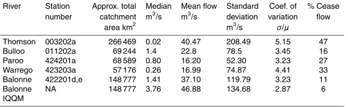
This study considers five river systems in south-western Queensland (SWQ), Australia (Table 2, Fig. 1). All of the river systems are similar, being terminal inland river sys-tems and intermittent in nature. Roughly, the average annual rainfall decreases in a 5

south westerly direction. With the exception of the Balonne, all of the river systems are unregulated. Streamflow in the Balonne River has been altered as a result of water extraction (Thoms and Parsons, 2003; Thoms, 2003) with most of the change occur-ring in flows with an average occurrence interval of less than 2 years (Thoms, 2003). Hence, an unimpaired dataset for this river was also used, which was provided by the 10

Department of Environment and Resources Management in Queensland Australia and was created using the Integrated Quality Quantity Model (IQQM) (Hameed and Podger, 2001). Throughout this study, streamflow is given as cubic meters per second (m3/s).

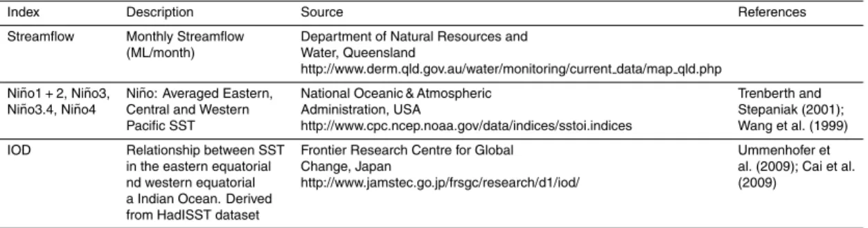
Sea surface temperature (SST) data can be readily obtained from several organisa-tions (Table 3). These datasets are usually a combination of spatially averaged monthly 15

temperature in degrees Celsius for various regions of the ocean (Fig. 2) (Wang et al., 1999). For ease of reading the regression formulas, Ni ˜no1+2 is referred to as Ni ˜no1.2. The IOD is the difference between SST in the western and eastern equatorial Indian Ocean (Fig. 3).

Climate datasets prior to 1959 were not considered due to recognised poor data 20

(6)

HESSD

8, 681–713, 2011

Title Page

Tables Figures

◭ ◮

Back Close

Full Screen / Esc

Discussion

P

a

per

|

Dis

cussion

P

a

per

|

Discussion

P

a

per

|

Discussio

n

P

a

per

|

2.2 Models

Modelling zero and non-zero data separately is equivalent to modelling streamflow using a zero-adjusted distribution of the type:

f(y θ, π) =

(1 − π) ify ₌ 0

π fT(y, θ) ify > 0

(1)

whereπis the probability of the occurrence of non-zero flow andfT(y,θ) is the

distribu-5

tion of the non-zero flow. Hence, initially the occurrence of monthly flow was modelled, for which the results are discussed in Sect. 3.1. As the outcome is binary, a binomial distribution was used (Hyndman and Grunwald, 2000). As a second step, the inten-sities (volumes) of the non-zero flows are modelled and the results are discussed in Sect. 3.2.

10

For the binomial model of the occurrence of flow, the following generalized linear model (GLM) can be initially specified

g(π) = log

π 1 − π

= x′β (2)

Whereπ is the probability of occurrence of non-zero flow, x′is a vector of covariates,

g(π) is the logit link function andβis a vector of coefficients forx. For comparison, the

15

following GAMLSS was specified (because GAMLSS is an extension of GLM; Rigby and Stasinopoulos, 2001):

g(π) = log

π 1 − π

= x′β +

J

X

j=1

sj wj

(3)

wherex′βis a combination of linear estimators as in Eq. (2), wj forj=1, 2, ...,J are

covariates and sj for j= 1, 2, ..., J are smoothing terms. The addition of

smooth-20

(7)

HESSD

8, 681–713, 2011

Title Page

Tables Figures

◭ ◮

Back Close

Full Screen / Esc

Discussion

P

a

per

|

Dis

cussion

P

a

per

|

Discussion

P

a

per

|

Discussio

n

P

a

per

|

smoothing is based on penalised B-splines (Eilers and Marx, 1996). The degree of smoothing is selected automatically using penalized maximum likelihood in the gamlss package (Rigby and Stasinopoulos, 2005). The GAMLSS models were implemented using the gamlss function in the gamlss package within the open source program R (Stasinopoulos et al., 2009; R Development Core Team, 2008).

5

For the model of zero flow (Intensity) distribution the data was subset to non-zero flow values. The Box-Cox t distribution (BCT) was used in the modelling. This four-parameter flexible distribution (Rigby and Stasinopoulos, 2006), has been shown to be a good fit for non-zero flow data from the Balonne River (Heller et al., 2009) and a number of gauging stations located west of the Australian Capital Territory (Wang et al., 10

2009). In the BCT distribution ˆµis the median, ˆσis the scale parameter (approximately the coefficient of variation), ˆνis the skewness and ˆτis the kurtosis of the non-zero flows. The probability for flows above a flow thresholdccan be subsequently calculated as:

ˆ

p(flow_i > c) = πˆ_ip (Z > z_i) (4)

Where zi =σˆ1_iνˆ

c

ˆ

µ_i

νˆ

−1

, if ˆν6₌0 and Z∼tτˆ has a t distribution with ˆτ degrees of

15

freedom and where ˆπi is the fitted probability of flow occurring in theith month (Eq. 4)

and ˆµi, ˆσi, ˆν and ˆτ are the parameters of the fitted BCT distribution. The probability

(Eq. 5) can be calculated readily in the gamlss package as ˆπ_i [1−pBCT(c,µ,ˆ σ,ˆ ν,ˆ τ)]ˆ where pBCT is the cumulative distribution function for the BCT distribution (Rigby and Stasinopoulos, 2006). The results of the probability of exceeding a flow threshold are 20

discussed in Sect. 3.3.

2.3 Covariates

Because our interest is in a 1 year ahead forecast, this study only considered the 12-month lagged covariates as predictors (this means forecasts are based on SST 12 months prior). Water users in the regions expressed most interest in a 12-month 25

(8)

HESSD

8, 681–713, 2011

Title Page

Tables Figures

◭ ◮

Back Close

Full Screen / Esc

Discussion

P

a

per

|

Dis

cussion

P

a

per

|

Discussion

P

a

per

|

Discussio

n

P

a

per

|

Different lag times or combinations of different lag times may also be considered, but this is not further pursued in this paper.

For some models, we also considered including a synthetic temporal covariate Time, a sequence of consecutive numbers 1, ..., n, where n is the length of the dataset, in the models to account for unmeasurable or unknown non-stationarity in the data. 5

An example of this could be non-stationarity due to water extraction or as a result of climate change in Eastern Australia (McAlpine et al., 2007; Pitman and Perkins, 2008; Cai and Cowan, 2008; Chiew et al., 2009).

A problem with such covariates in forecasts is that the future relationship between the response variable and the covariate is unknown and that the relationship is strictly 10

empirical. We can only assume that the observed trend in the data continues for the next 12 months to be used in the forecast. However, the same is somewhat true for all relationships in a statistical model, but in contrast, for the SST covariates, we can assume that there is some underlying physical process which is captured by the statistical model. For a slowly varying smooth covariate the lack of knowledge about 15

future trends might also not be a concern, but for a rapidly changing covariate (or jump changes) it could be problematic.

The further synthetic variables cosine and sine are harmonic covariates and have been included to account for seasonal fluctuations in the data (Hyndman and Grun-wald, 2000):

20

sine = sin 2π Sm

12

cosine = cos 2π Sm

12

(5)

WhereSmism(mod 12) wheremis the month. Fitting higher order harmonics was not

deemed necessary due to the added flexibility of fitting these harmonic covariates with a penalised B-spline. Significance of these covariates indicate strong seasonal trends in the streamflow and thus capture seasonal climatic or within catchment processes. 25

(9)

HESSD

8, 681–713, 2011

Title Page

Tables Figures

◭ ◮

Back Close

Full Screen / Esc

Discussion

P

a

per

|

Dis

cussion

P

a

per

|

Discussion

P

a

per

|

Discussio

n

P

a

per

|

processes and seasonal variations (what would normally be the main focus of catch-ment hydrology) captured in the harmonic terms. The second layer is the oceanic influences modelled through the influence of the SST’s and the final layer consists of a long term trend or periodicity that can be modelled by a synthetic temporal variable.

2.4 Goodness of fit 5

To determine the most parsimonious model (the best model with the least number of covariates), a stepwise fitting method, the stepGAIC function, is used. This is based on the Generalized Akaike Information Criterion (GAIC), which is a model selection criterion where GAIC₌−2L₊kN, L is the log likelihood, k is the penalty parameter and N is the number of parameters in the fitted model (Akaike, 1974). A value of 10

k=3 delivered the highest skill of models selected using stepGAIC after a test with di_fferent values fromk₌2 tok₌log(n), also known as the Schwarz Bayesian Criteria, wherenis the length of the dataset. The stepGAIC process also selects whether or not B-splines are fitted to the covariates. Hence, it is quite possible that the most parsimonious model is simply a GLM.

15

For all fitted models residuals were checked for independence and identical distribu-tion.

Validation of the models was conducted using a leave 12 month out cross validation routine similar to that suggested by Chowdhury and Sharma (2009). Essentially, this involved leaving one year of data out in each model run and then using the left out 20

data for the final forecast. Forecast skill was then calculated based on the combined forecasts.

The Brier Skill Score (BSS) and Relative Operating Characteristic (ROC) are the most common means for verifying probabilistic forecasts (Jolliffe and Stephenson, 2003; Wilks, 2006). These were implemented in the verification package in R (NCAR, 25

(10)

HESSD

8, 681–713, 2011

Title Page

Tables Figures

◭ ◮

Back Close

Full Screen / Esc

Discussion

P

a

per

|

Dis

cussion

P

a

per

|

Discussion

P

a

per

|

Discussio

n

P

a

per

|

to be significant. Typical BSS values for forecasts of daily streamflow in a temperate cli-mate lie between 0.6 and 0.8 at day one and decrease to between 0 and 0.2 at day 10 (Roulin and Vannitsem, 2005). Similarly, BSS values of between 0 and 0.5 were found in Iowa (USA) using monthly ensemble streamflow prediction (Hashino et al., 2006).

3 Results and discussion 5

3.1 Occurrence model

Typical examples of the fitted models for the occurrence of non-zero flows for SWQ Rivers are given in Table 4.

The Pacific Ocean SST affects the strength of the northern Australian monsoon and cyclonic activity over a year (Evans and Allan, 1992). From Table 4, it is clear that the 10

Pacific Ocean SSTs are the dominant drivers of the probability of occurrence of zero streamflow in most of the rivers. Local knowledge suggest that cyclonic activity close to, or crossing, the coast in north eastern Australia is often indicative of significant streamflow in the study region with a delay of up to a number of months. In general, the relationship between Pacific Ocean SST and streamflow is linear. Except for the 15

Balonne IQQM data, the relationship between the eastern and the western and central Pacific SST are of opposite sign. This may be explained by the fact that changes in SST in the central and western pacific and the eastern Pacific are phase shifted to varying degrees (Wang et al., 2010). Finally, streamflow in the Balonne River, which has one of its two major sources further south west than the other catchments, is 20

significantly affected by Indian Ocean dipole. It has been shown that IOD is linked with the development of northwest cloudbands (Verdon and Franks, 2005a) which in turn can bring winter rainfall to central and Eastern Australia (Braganza, 2008; Courtney, 1998; Collins, 1999).

The inclusion of a Time covariate for the Balonne (observed streamflow) river model 25

(11)

HESSD

8, 681–713, 2011

Title Page

Tables Figures

◭ ◮

Back Close

Full Screen / Esc

Discussion

P

a

per

|

Dis

cussion

P

a

per

|

Discussion

P

a

per

|

Discussio

n

P

a

per

|

of the gauging station. The model indicates that post 1980, the probability of observed flow occurring in the Balonne is decreasing in time (Fig. 4). This would suggest that increased water extraction occurred post 1980 upstream of the gauging station (Thoms, 2003; Thoms and Parsons, 2003). Rather than using a Time variable it would make more sense to include actual extraction volumes or at least a function representing 5

extraction rules as a covariate. However, due to the sensitive nature of this data, this has not been made available.

The forecast skill is significant at all gauging stations with the Thomson showing the greatest skill (Table 5).

3.2 Intensity model 10

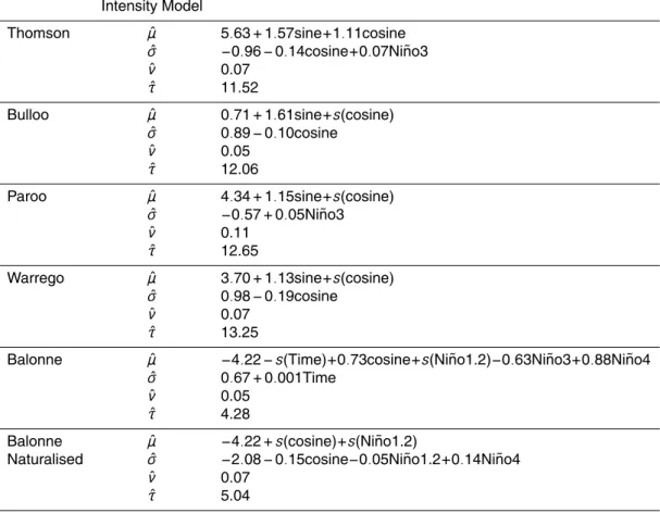
The intensity model gives the probability of the level of non-zero monthly flow above a threshold. It therefore predicts the distribution of monthly flow values (Table 6).

From Table 6, it is clear that SST is less important in the intensity models and in-stead the two harmonic terms explain much of the variation in each model for non-zero streamflow. This would indicate that for the actual intensity of flow internal catchment 15

processes and seasonal climate influences are more important than longer range tele-connections for non-zeroflows. However, SSTs do have some influence on the scale parameter ˆσ, indicating a positive relationship between central and eastern SST and streamflow variability. There is some spatial and temporal heterogeneity in the rela-tionships between SST and streamflow between the regions. This is the result of the 20

(12)

HESSD

8, 681–713, 2011

Title Page

Tables Figures

◭ ◮

Back Close

Full Screen / Esc

Discussion

P

a

per

|

Dis

cussion

P

a

per

|

Discussion

P

a

per

|

Discussio

n

P

a

per

|

3.3 Probabilistic forecast of streamflow

Using Eq. (5), the probability of getting at least the median and the mean flow was cal-culated for each river. The forecasts for all of the gauging stations show significant skill (Table 7). Essentially, in both cases, the forecasts perform better than only using the median or mean values. As with the occurrence model, the forecast for the Thomson 5

gauging station shows the greatest skill. Using the Thomson as an example, another way of looking at this result is to say that if you use the forecast for your decision mak-ing, you would expect a 35% improvement over basing your decision on the median flow of each month. A further important observation is that as the flow threshold in-creases (from median to mean in this case) the value for BSS dein-creases suggesting 10

that as the flow threshold increases the system becomes less easy to forecast. A logical reason for this observation is that at the higher flow thresholds the number of observed flows decreases, adding to the decrease in the forecast skill.

From Table 7 and Eq. (5) it is easy to derive a forecast monthly flow duration curve 12 months ahead in time by generating regularly spaced flow threshold values up to 15

a maximum threshold, say the maximum recorded flow (Fig. 5). The advantage of presenting forecasts as a flow duration curve is that they are already used by water managers to determine water extraction rates, irrigators for irrigation planning and by biologists to determine environmental flows (Acreman, 2005; Cigizoglu and Bayazit, 2000). Aside from the Thomson River, the forecast probability of flow is systematically 20

overestimated for the other river systems (Fig. 5). The reason for this is that the Box-Cox t distribution is not capturing all the skewness in these datasets and thus cannot generate the full range of probabilities.

4 General discussion

This study has demonstrated the ability of flexible statistical models to make skilful 25

(13)

HESSD

8, 681–713, 2011

Title Page

Tables Figures

◭ ◮

Back Close

Full Screen / Esc

Discussion

P

a

per

|

Dis

cussion

P

a

per

|

Discussion

P

a

per

|

Discussio

n

P

a

per

|

absence of detailed understanding of complex large semi-arid catchments, statistical approaches, such as the demonstrated GAMLSS framework o_ffer advantages over de-terministic and conceptual catchment models for forecasts. From an explanatory view, the work has highlighted the dominance of the Pacific Ocean SST on the occurrence of monthly flows in these catchments, increasing our understanding of these climatic 5

drivers on Eastern Australian streamflow. In addition, in relation to the complex layers of the catchments, it is clear that for the occurrence of monthly flow the larger scale climatic layer is influential, while for the intensity of monthly flow local catchment pro-cesses and seasonal variation dominate. However, SST does influence the year to year variability of the non-zero monthly flows. The temporal covariate Time gives important 10

explanations of long term trends (such as the decrease in the observed Balonne flows). As this study is primarily a demonstration of a method, there is great scope for fu-ture work building on this approach for forecasting both streamflow and rainfall. For example, we have not considered antecedent soil moisture as a covariate in the model (Timbal et al., 2002) as this is relatively unworkable for the long range forecasts con-15

sidered here. However, for shorter range forecasts, this could easily be introduced in the catchment process layer by incorporating a covariate based on the number of days or months from the start of a dry spell derived from local daily flow or rainfall records (Sharma and Lall, 1998). Furthermore, we have only used a small selection of available climate indices and we have only considered a single lag of 12 months 20

which could be extended to incorporate multiple lags or shorter lags for shorter range or seasonal forecasts. Examples of other indices which have been shown to be useful for forecasting precipitation or streamflow in Australia are the Tropical Indo-Pacific ther-mocline (Ruiz et al., 2007) and the Southern Annular Mode (Meneghini et al., 2007). The methodology can also be used to identify temporal and spatial patterns in tele-25

(14)

HESSD

8, 681–713, 2011

Title Page

Tables Figures

◭ ◮

Back Close

Full Screen / Esc

Discussion

P

a

per

|

Dis

cussion

P

a

per

|

Discussion

P

a

per

|

Discussio

n

P

a

per

|

have been considered in this study and it is expected that forecast will improve if other distributions are considered. In particular, it would be expected that using mixture dis-tributions (Stasinopoulos and Rigby, 2007) for the intensity of streamflow will improve forecast skill. This is part of our ongoing research.

5 Conclusions 5

Using a GAMLSS regression framework it is possible to make a skilful forecast of the probability of monthly streamflow occurring 1 year (12 months) ahead in highly variable intermittent streams catchments in the inland regions of eastern Australia where only streamflow data is available. The GAMLSS framework is able to cope with non-linearity in the relationships between SST and monthly streamflow, which leads to superior 10

model performance compared with more traditional linear models. Furthermore, in the absence of more detailed data and using synthetic covariates, it is possible to account for non-stationarity and seasonality in the data in an explanatory framework. The model output is probabilistic and hence the results can be presented as the well known flow duration curve. This output can be used by irrigators, graziers and natural resource 15

management staffto aid in decision making in these highly variable environments.

(15)

HESSD

8, 681–713, 2011

Title Page

Tables Figures

◭ ◮

Back Close

Full Screen / Esc

Discussion

P

a

per

|

Dis

cussion

P

a

per

|

Discussion

P

a

per

|

Discussio

n

P

a

per

|

References

Abawi, Y., Dutta, S., Zhang, X., and McClymont, D.: ENSO-based streamflow forecasting and its application to water allocation and cropping decisions-an Australian experience, Regional hydrological impacts of climate change-Impact assessment and decision making, Brazil, 346–354, 2005.

5

Acreman, M.: Linking science and decision-making: features and experience from environmen-tal river flow setting, Environ. Modell. Softw., 20, 99–109, 2005.

Akaike, H.: A new look at the statistical model identification, IEEE T. Automat. Contr., 19, 716– 723, 1974.

Alves, O., Wang, G., Zhong, A., Smith, N., Tzeitkin, F., Warren, G., Schiller, A., Godfrey, S., and

10

Meyers, G.: POAMA: Bureau of Meteorology operational coupled model seasonal forecast system, Proceedings of the ECMWF Workshop on the Role of the Upper Ocean in Medium and Extended Range Forecasting, Reading, UK, 22–32, 2002,.

Barry, S. C. and Welsh, A. H.: Generalized additive modelling and zero inflated count data, Ecol. Modell., 157, 179–188, 2002.

15

Berg, D.: Bankruptcy prediction by generalized additive models, Appl. Stoch. Model. Bus., 23, 129–143, 2007.

Braganza, K.: Seasonal climate summary southern hemisphere (autumn 2007): La Ni ˜na emerges as a distinct possibility in 2007, Australian Meteorological Magazine, 57, 2008. Brown, B. G., Katz, R. W., and Murphy, A. H.: On the economic value of seasonal-precipitation

20

forecasts: the fallowing/planting problem, B. Am. Meteorol. Soc., 67, 833–841, 1986. Buizza, R.: The value of probabilistic prediction, Atmos. Sci. Lett., 9, 36–42, 2008.

Cai, W. and Cowan, T.: Evidence of impacts from rising temperature on inflows to the Murray-Darling Basin, Geophys. Res. Lett., 35, L07701, doi:10.1029/2008GL033390, 2008.

Cai, W., Cowan, T., and Sullivan, A.: Recent unprecedented skewness towards positive Indian

25

Ocean Dipole occurrences and its impact on Australian rainfall, Geophys. Res. Lett., 36, L011705, doi:10.1029/2009GL037604, 2009.

Chiew, F. H. S., Piechota, T. C., Dracup, J. A., and McMahon, T. A.: El Nino/Southern Oscillation and Australian rainfall, streamflow and drought: Links and potential for forecasting, J. Hydrol., 192, 138–149, 1998.

30

(16)

HESSD

8, 681–713, 2011

Title Page

Tables Figures

◭ ◮

Back Close

Full Screen / Esc

Discussion

P

a

per

|

Dis

cussion

P

a

per

|

Discussion

P

a

per

|

Discussio

n

P

a

per

|

Chiew, F. H. S., Teng, J., Vaze, J., Post, D. A., Perraud, J. M., Kirono, D. G. C., and Viney, N. R.: Estimating climate change impact on runoff across southeast Australia: Method, results, and implications of the modeling method, Water Resour. Res., 45, W10414, doi:10.1029/2008WR007338, 2009.

Chowdhury, S. and Sharma, A.: Multisite seasonal forecast of arid river flows

us-5

ing a dynamic model combination approach, Water Resour. Res., 45, W10428, doi:10.1029/2008WR007510, 2009.

Cigizoglu, H. K. and Bayazit, M.: A generalized seasonal model for flow duration curve, Hydrol. Process., 14, 1053–1067, 2000.

Collins, D.: Seasonal climate summary southern hemisphere (winter 1998): transition toward a

10

cool episode (La Ni ˜na), Australian Meteorological Magazine, 48, 1999.

Cordery, I.: Long range forecasting of low rainfall, Int. J. Climatol., 19, 463–470, 1999.

Courtney, J.: Seasonal climate summary southern hemisphere (autumn 1998): decline of a warm episode (El Ni ˜no), Australian Meteorological Magazine, 47, 1998.

De Jong, P. and Heller, G. Z.: Generalized linear models for insurance data, in: International

15

Series on Actuarial Science, edited by: Davis, M., Hylands, J., McCutcheon, J., Norberg, R., Panjer, H., and Wilson, A., Cambridge University Press, New York, USA, 2008.

Dettinger, M. D. and Diaz, H. F.: Global characteristics of streamflow seasonality and variability, J. Hydrometeorol., 1, 289–310, 2000.

Dutta, S. C., Ritchie, J. W., Freebairn, D. M., and Abawi, Y.: Rainfall and streamflow response

20

to El Nino Sothern Oscillation: a case study in a semiarid catchment, Australia, Hydrolog. Sci. J., 51, 1006–1020, 2006.

Eilers, P. H. C. and Marx, B. D.: Flexible smoothing with B-splines and penalties, Stat. Sci., 11, 89–101, 1996.

Evans, J. L. and Allan, R. J.: El Ni ˜no/Southern Oscillation modification to the structure of the

25

monsoon and tropical cyclone activity in the Australasian region, Int. J. Climatol., 12, 611– 623, 1992.

Faraway, J. and Chatfield, C.: Time series forecasting with neural networks: a comparative study using the airline data, Appl. Stat., 47, 231–250, 1998.

Grunwald, G. K. and Jones, R. H.: Markov models for time series with mixed distribution,

30

Environmentrics, 11, 327–339, 2000.

(17)

HESSD

8, 681–713, 2011

Title Page

Tables Figures

◭ ◮

Back Close

Full Screen / Esc

Discussion

P

a

per

|

Dis

cussion

P

a

per

|

Discussion

P

a

per

|

Discussio

n

P

a

per

|

Hameed, T. and Podger, G.: Use of the IQQM simulation model for planning and management of a regulated river system, in: Integrated Water Resources Management, edited by: Marino, M. A. and Simonovic, S. P., IAHS 83-90, 83–90, 2001.

Hamill, T. M. and Wilks, D. S.: A probabilistic forecast contest and the difficulty in assessing short-range forecast uncertainty, Weather Forecast., 10, 620–631, 1995.

5

Hashino, T., Bradley, A. A., and Schwartz, S. S.: Evaluation of bias-correction methods for ensemble streamflow volume forecasts, Evaluation, 3, 561–594, 2006.

Hastie, T. and Tibshirani, R.: Generalized additive models (with discussion), Stat. Sci., 1, 297– 310, 1986.

Hayman, P., Crean, J., Mullen, J., and Parton, K.: How do probabilistic seasonal climate

fore-10

casts compare with other innovations that Australian farmers are encouraged to adopt?, Aust. J. Agr. Res., 58, 975–984, 2007.

Heller, G. Z., Stasinopoulos, D. M., Rigby, R. A., and Van Ogtrop, F. F.: Randomly stopped sum models: a hydrological application, 24th International Workshop on Statistical Modelling, New York, 2009.

15

Hyndman, R. J. and Grunwald, G. K.: Generalized additive modelling of mixed distribution markov models with application to Melbourne’s rainfall, Aust. Nz. J. Stat., 42, 145–158, 2000. Jolliffe, I. T. and Stephenson, D. B.: Forecast verification: a practitioner’s guide in atmospheric

science, edited by: Jolliffe, I. T. and Stephenson, D. B., Wiley, Wiltshire, 2003.

Kiem, A. S. and Verdon-Kidd, D. C.: Climatic Drivers of Victorian Streamflow: Is ENSO the

20

Dominant Influence?, Aust. J. Water Resour., 13, 17–29, 2009.

Krzysztofowicz, R.: Why should a forecaster and a decision maker use Bayes theorem, Water Resour. Res., 19, 327–336, 1983.

Krzysztofowicz, R.: The case for probabilistic forecasting in hydrology, J. Hydrol., 249, 2–9, 2001.

25

Lachenbruch, P. A.: Comparisons of two-part models with competitors, Stat. Med., 20, 1215– 1234, 2001.

Mason, S. and Graham, N.: Areas beneath the relative operating characteristics (roc) and relative operating levels (rol) curves: Statistical significance and interpretation, Q. J. Roy. Meteor. Soc., 128, 2145–2166, 2002.

30

(18)

HESSD

8, 681–713, 2011

Title Page

Tables Figures

◭ ◮

Back Close

Full Screen / Esc

Discussion

P

a

per

|

Dis

cussion

P

a

per

|

Discussion

P

a

per

|

Discussio

n

P

a

per

|

Meneghini, B., Simmonds, I., and Smith, I. N.: Association between Australian rainfall and the Southern Annular Mode, Int. J. Climatol., 27, 109–121, 2007.

Milly, P. C. D., Betancourt, J., Falkenmark, M., Hirsch, R. M., Kundzewicz, Z. W., Lettenmaier, D. P., and Stouffer, R. J.: Stationarity is dead: whither water management?, Science, 319, 573–574, 2008.

5

Mjelde, J. W., Sonka, S. T., Dixon, B. L., and Lamb, P. J.: Valuing forecast characteristics in a dynamic agricultural production system, Am. J. Agr. Econ., 70, 674–684, 1988.

Pappenberger, F. and Beven, K. J.: Ignorance is bliss: Or seven reasons not to use uncertainty analysis, Water Resour. Res., 42, W05302, doi:10.1029/2005WR004820, 2006.

Piechota, T. C. and Dracup, J. A.: Long-range streamflow forecasting using El Nino-Southern

10

Oscillation indicators, J. Hydrol. Eng., 4, 144–151, 1999.

Piechota, T. C., Chiew, F. H. S., Dracup, J. A., and McMahon, T. A.: Seasonal streamflow forecasting in eastern Australia and the El Ni ˜no-Southern Oscillation, Water Resour. Res., 34, 3035–3044, 1998.

Piechota, T. C., Chiew, F. H. S., Dracup, J. A., and McMahon, T. A.: Development of exceedance

15

probability streamflow forecast, J. Hydrol. Eng., 6, 20–28, 2001.

Pitman, A. J. and Perkins, S. E.: Regional projections of future seasonal and annual changes in rainfall and temperature over Australia based on skill-selected AR4 models, Earth Interact., 12, Paper No. 12, 2008.

Rigby, R. and Stasinopoulos, D.: The GAMLSS project: a flexible approach to statistical

mod-20

elling, in: New Trends in Statistical Modelling: Proceedings of the 16th International Work-shop on Statistical Modelling, edited by: Klein, B. and Korsholm, L., Odense, Denmark, 249–256, 2001.

Rigby, R. A. and Stasinopoulos, D. M.: Generalized additive models for location, scale and shape (with discussion), J. Roy. Stat. Soc. Ser. C, 54, 507–554, 2005.

25

Rigby, R. A. and Stasinopoulos, D. M.: Using the Box-Cox t distribution in GAMLSS to model skewness and kurtosis, Stat. Model., 6, 209–229, 2006.

Roulin, E. and Vannitsem, S.: Skill of medium-range hydrological ensemble predictions, J. Hydrometeorol., 6, 729–744, 2005.

Ruiz, J. E., Cordery, I., and Sharma, A.: Forecasting streamflows in Australia using the tropical

30

Indo-Pacific thermocline as predictor, J. Hydrol., 341, 156–164, 2007.

(19)

HESSD

8, 681–713, 2011

Title Page

Tables Figures

◭ ◮

Back Close

Full Screen / Esc

Discussion

P

a

per

|

Dis

cussion

P

a

per

|

Discussion

P

a

per

|

Discussio

n

P

a

per

|

Schwarzer, G., Vach, W., and Schumacher, M.: On the misuses of artificial neural networks for prognostic and diagnostic classification in oncology, Stat. Med., 19, 541–561, 2000.

Sharma, A. and Lall, U.: A nonparametric approach for daily rainfall simulation, Math. Comput. Simulat., 48, 361–372, 1998.

Sharma, A., Luk, K. C., Cordery, I., and Lall, U.: Seasonal to interannual rainfall probabilistic

5

forecasts for improved water supply management: Part 2 – Predictor identification of quar-terly rainfall using ocean-atmosphere information, J. Hydrol., 239, 240–248, 2000.

Stasinopoulos, D. and Rigby, R.: Generalized additive models for location scale and shape (GAMLSS) in R, J. Stat. Softw., 23, 1–46, 2007.

Thoms, M. C.: Floodplain-river ecosystems: lateral connections and the implications of human

10

interference, Geomorphology, 56, 335–349, 2003.

Thoms, M. C. and Parsons, M.: Identifying spatial and temporal patterns in the hydrological character of the Condamine-Balonne river, Australia, using multivariate statistics, River Res. Appl., 19, 443–457, 2003.

Timbal, B., Power, S., Colman, R., Viviand, J., and Lirola, S.: Does soil moisture influence

15

climate variability and predictability over Australia?, J. Climate, 15, 1230–1238, 2002. Ummenhofer, C. C., England, M. H., McIntosh, P. C., Meyers, G. A., Pook, M. J., Risbey, J.

S., Gupta, A. S., and Taschetto, A. S.: What causes southeast Australia’s worst droughts?, Geophys. Res. Lett., 36, L04706, doi:10.1029/2008GL036801, 2009.

Verdon, D. C. and Franks, S. W.: Indian Ocean sea surface temperature variability and winter

20

rainfall: Eastern Australia, Water Resour. Res., 41, W09413, doi:10.1029/2004WR003845, 2005a.

Verdon, D. C. and Franks, S. W.: Influence of Indian Ocean sea-surface temperature variability on winter rainfall across eastern Australia, Regional Hydrological Impacts of Climatic Change – Impact assessment and decision making, Brazil, 335–345, 2005b.

25

Wang, C., Weisberg, R. H., and Virmani, J. I.: Western pacific interannual variability associated with the El Nino-Southern Oscillation, J. Geophys. Res., 104, 5131–5149, 1999.

Wang, G. and Hendon, H. H.: Sensitivity of Australian rainfall to Inter – El Ni ˜no variations, J. Climate, 20, 4211–4226, 2007.

Wang, Q. J., Robertson, D. E., and Chiew, F. H. S.: A Bayesian joint probability modeling

30

(20)

HESSD

8, 681–713, 2011

Title Page

Tables Figures

◭ ◮

Back Close

Full Screen / Esc

Discussion

P

a

per

|

Dis

cussion

P

a

per

|

Discussion

P

a

per

|

Discussio

n

P

a

per

|

Wang, S. Y., Gillies, R. R., Hipps, L. E., and Jin, J.: A transition-phase teleconnection of the Pacific quasi-decadal oscillation, Clim. Dynam., 37, 1–13, 2010.

White, B.: The Australian experience, in: Applications of seasonal climate forecasting in agri-culture and natural ecosystems, edited by: Hammer, G. L., Nicholls, N., and Mitchell, C., Kluwer, Dordercht, 1–22, 2000.

5

Wilks, D. S.: Statistical methods in the atmospheric sciences, in: International Geophysics, edited by: Dmowska, R., Hartman, D., and Rossby, T. H., Elsevier, San Diego, 2006.

Wilks, D. S. and Murphy, A. H.: A decision-analytic study of the joint value of seasonal precip-itation and temperature forecasts in a choice-of-crop problem, Atmos.-Ocean, 24, 353–368, 1986.

10

Wood, S. N.: Generalized additive models An introduction with R, in: Statistical Science Series, edited by: Carlin, B. P., Chatfield, C., Tanner, M., and Zidek, J., Chapman and Hall/CRC, Boca Raton, 2006.

Wooldridge, S. A., Franks, S. W., and Kalma, J. D.: Hydrological implications of the Southern Oscillation: variability of the rainfall-runoffrelationship, Hydrolog. Sci. J., 46, 73–88, 2001.

15

(21)

HESSD

8, 681–713, 2011

Title Page

Tables Figures

◭ ◮

Back Close

Full Screen / Esc

Discussion

P

a

per

|

Dis

cussion

P

a

per

|

Discussion

P

a

per

|

Discussio

n

P

a

per

|

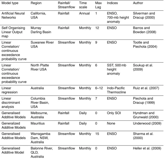
Table 1.Summary of statistical models used for forecasting rainfall and streamflow.

Model type Region Rainfall/ Time Max Indices Author

Streamflow scale Lag

Artificial Neural California, Rainfall Annual 1 ENSO, Silverman and

Networks USA 700-mb height Dracup (2000)

anomaly

Self Organising Murray Rainfall Monthly 12 ENSO Barros and

Linear Output Darling Basin Bowden (2008)

map

Linear Suwanee River Streamflow Monthly 9 ENSO Tootle and

Correlation/ USA Piechota (2004)

continuous exceedance probability curve

Linear North Platte Streamflow Monthly 6 SST, 500 mb Soukup et al.

Correlation/ River USA height (2009)

continuous anomaly

exceedance probability curve

Linear Australia Streamflow Monthly 6–12 Indo-Pacific Ruiz et al. (2007)

regression Thermocline

Linear Columbia Streamflow Monthly 7 ENSO Piechota and

discriminant River Basin, Dracup (1999)

analysis USA

Generalised Melbourne, Rainfall Daily 0 Only SOI Hyndman and

Additive Models Australia Grunwald (2000)

Generalized Mauritius Rainfall Daily 0 None Underwood (2009)

Additive Models

Generalised Warragamba Streamflow Monthly 15 ENSO Sharma et al.

Additive Models Dam, NSW, (2000)

Australia

Generalised Balonne River, Streamflow Monthly 0 ENSO Heller et al. (2009) Additive Model QLD,

(22)

HESSD

8, 681–713, 2011

Title Page

Tables Figures

◭ ◮

Back Close

Full Screen / Esc

Discussion

P

a

per

|

Dis

cussion

P

a

per

|

Discussion

P

a

per

|

Discussio

n

P

a

per

|

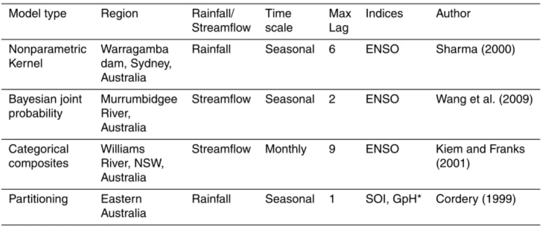
Table 1.Continued.

Model type Region Rainfall/ Time Max Indices Author

Streamflow scale Lag

Nonparametric Warragamba Rainfall Seasonal 6 ENSO Sharma (2000)

Kernel dam, Sydney,

Australia

Bayesian joint Murrumbidgee Streamflow Seasonal 2 ENSO Wang et al. (2009) probability River,

Australia

Categorical Williams Streamflow Monthly 9 ENSO Kiem and Franks

composites River, NSW, (2001)

Australia

Partitioning Eastern Rainfall Seasonal 1 SOI, GpH* Cordery (1999)

Australia

(23)

HESSD

8, 681–713, 2011

Title Page

Tables Figures

◭ ◮

Back Close

Full Screen / Esc

Discussion

P

a

per

|

Dis

cussion

P

a

per

|

Discussion

P

a

per

|

Discussio

n

P

a

per

|

Table 2.Flow statistics for south western Queensland Rivers.

River Station Approx. total Median Mean flow Standard Coef. of % Cease number catchment m3/s m3/s deviation variation flow

area km2 m3/s σ/µ

Thomson 003202a 266 469 0.02 40.47 208.49 5.15 47

Bulloo 011202a 69 244 1.4 22.8 78.5 3.45 16

Paroo 424201a 68 589 0.80 16.20 52.30 3.23 27

Warrego 423203a 57 176 0.26 16.99 74.87 4.41 33

Balonne 422201d,e 148 777 1.41 37.10 119.79 3.23 11

Balonne NA 148 777 3.76 46.88 134.68 2.87 6

(24)

HESSD

8, 681–713, 2011

Title Page

Tables Figures

◭ ◮

Back Close

Full Screen / Esc

Discussion

P

a

per

|

Dis

cussion

P

a

per

|

Discussion

P

a

per

|

Discussio

n

P

a

per

|

Table 3.Summary of data used and availability.

Index Description Source References

Streamflow Monthly Streamflow Department of Natural Resources and (ML/month) Water, Queensland

http://www.derm.qld.gov.au/water/monitoring/current data/map qld.php

Ni ño1+2, Ni ño3, Ni ño: Averaged Eastern, National Oceanic & Atmospheric Trenberth and Ni ño3.4, Ni ño4 Central and Western Administration, USA Stepaniak (2001);

Pacific SST http://www.cpc.ncep.noaa.gov/data/indices/sstoi.indices Wang et al. (1999) IOD Relationship between SST Frontier Research Centre for Global Ummenhofer et

in the eastern equatorial Change, Japan al. (2009); Cai et al. nd western equatorial http://www.jamstec.go.jp/frsgc/research/d1/iod/ (2009)

(25)

HESSD

8, 681–713, 2011

Title Page

Tables Figures

◭ ◮

Back Close

Full Screen / Esc

Discussion

P

a

per

|

Dis

cussion

P

a

per

|

Discussion

P

a

per

|

Discussio

n

P

a

per

|

Table 4.Occurrence models for river systems in south western Queensland. In these formulas

ˆ

πis the fitted probability of occurrence of flow, Time is a sequence 1, 2, 3, ...,nands() is a penalised B-spline smooth function. The other covariates are as described in Table 3.

River Gauge Station number Occurrence model

Thomson 003202a log πˆ

1−πˆ

=7.05₊1.18sine₊0.73Ni ño1.2₊s(Ni ño3)₊s(Ni ño4)

Bulloo 011202a log πˆ

1−πˆ

=6.13+0.38Ni ˜no1.2+s(Ni ˜no4)

Paroo 424201a log₁₋πˆ_π_ˆ=1.09+0.97sine

Warrego 423203a log πˆ

1−πˆ

=−0.83+0.54Ni ˜no1.2−0.42Ni ˜no3

Balonne 422201d and e log₁₋πˆ_π_ˆ=29.52+s(Time)+s(sine)−0.92Ni ˜no4+0.49IOD

Balonne IQQM NA log πˆ

1−πˆ

(26)

HESSD

8, 681–713, 2011

Title Page

Tables Figures

◭ ◮

Back Close

Full Screen / Esc

Discussion

P

a

per

|

Dis

cussion

P

a

per

|

Discussion

P

a

per

|

Discussio

n

P

a

per

|

Table 5.Forecast skill for the occurrence model at the five gauging stations and naturalised

data.

Thomson Bulloo Paroo Warrego Balonne Balonne Naturalised

BSS 0.34 0.09 0.08 0.14 0.15 0.05

(27)

HESSD

8, 681–713, 2011

Title Page

Tables Figures

◭ ◮

Back Close

Full Screen / Esc

Discussion

P

a

per

|

Dis

cussion

P

a

per

|

Discussion

P

a

per

|

Discussio

n

P

a

per

|

Table 6.Intensity models for river systems in south western Queensland. Here ˆµis the median,

ˆ

σis the scale parameter (approximately the coefficient of variation), ˆνis the skewness and ˆτis the kurtosis in the BCT distribution of the non-zero flows.

Intensity Model

Thomson µˆ 5.63+1.57sine+1.11cosine ˆ

σ −0.96−0.14cosine+0.07Ni ˜no3 ˆ

ν 0.07

ˆ

τ 11.52

Bulloo µˆ 0.71+1.61sine+s(cosine)

ˆ

σ 0.89−0.10cosine ˆ

ν 0.05

ˆ

τ 12.06

Paroo µˆ 4.34+1.15sine+s(cosine)

ˆ

σ −0.57+0.05Ni ˜no3 ˆ

ν 0.11

ˆ

τ 12.65

Warrego µˆ 3.70+1.13sine+s(cosine) ˆ

σ 0.98−0.19cosine ˆ

ν 0.07

ˆ

τ 13.25

Balonne µˆ −4.22−s(Time)+0.73cosine+s(Ni ño1.2)−0.63Ni ño3+0.88Ni ño4 ˆ

σ 0.67+0.001Time

ˆ

ν 0.05

ˆ

τ 4.28

Balonne µˆ −4.22+s(cosine)+s(Ni ˜no1.2)

Naturalised σˆ −2.08−0.15cosine−0.05Ni ˜no1.2+0.14Ni ˜no4 ˆ

ν 0.07

ˆ

(28)

HESSD

8, 681–713, 2011

Title Page

Tables Figures

◭ ◮

Back Close

Full Screen / Esc

Discussion

P

a

per

|

Dis

cussion

P

a

per

|

Discussion

P

a

per

|

Discussio

n

P

a

per

|

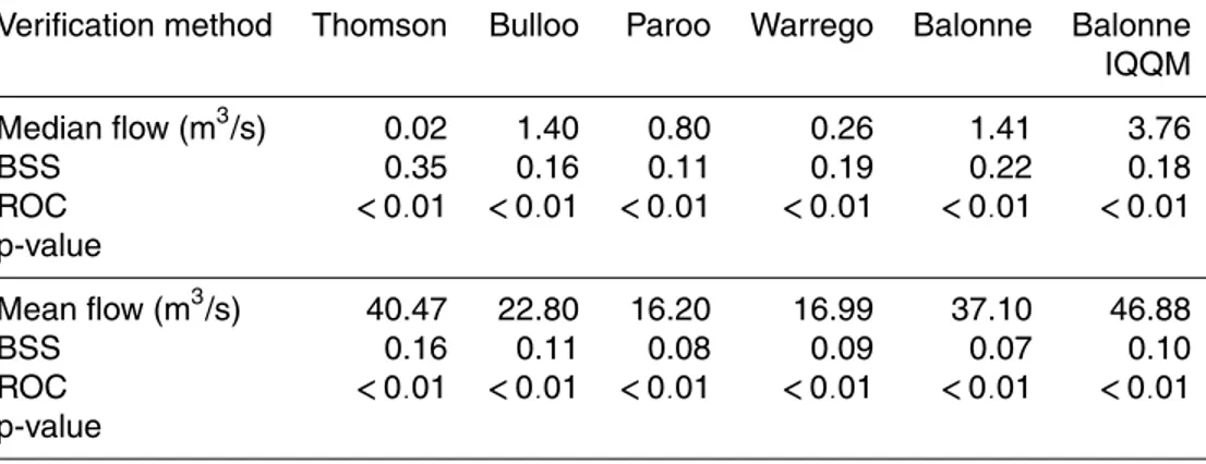
Table 7.Forecast skill for the intensity model at the five gauging stations and naturalised data.

Verification method Thomson Bulloo Paroo Warrego Balonne Balonne IQQM Median flow (m3/s) 0.02 1.40 0.80 0.26 1.41 3.76

BSS 0.35 0.16 0.11 0.19 0.22 0.18

ROC <0.01 <0.01 <0.01 <0.01 <0.01 <0.01 p-value

Mean flow (m3/s) 40.47 22.80 16.20 16.99 37.10 46.88

BSS 0.16 0.11 0.08 0.09 0.07 0.10

(29)

HESSD

8, 681–713, 2011

Title Page

Tables Figures

◭ ◮

Back Close

Full Screen / Esc

Discussion

P

a

per

|

Dis

cussion

P

a

per

|

Discussion

P

a

per

|

Discussio

n

P

a

per

|

(30)

HESSD

8, 681–713, 2011

Title Page

Tables Figures

◭ ◮

Back Close

Full Screen / Esc

Discussion

P

a

per

|

Dis

cussion

P

a

per

|

Discussion

P

a

per

|

Discussio

n

P

a

per

|

Fig. 2. Locations of average sea surface temperature locations for Ni ˜no 1, 2, 3, 3.4 and 4

(31)

HESSD

8, 681–713, 2011

Title Page

Tables Figures

◭ ◮

Back Close

Full Screen / Esc

Discussion

P

a

per

|

Dis

cussion

P

a

per

|

Discussion

P

a

per

|

Discussio

n

P

a

per

|

Fig. 3. Locations of average sea surface temperature locations for IOD (source: Bureau of

(32)

HESSD

8, 681–713, 2011

Title Page

Tables Figures

◭ ◮

Back Close

Full Screen / Esc

Discussion

P

a

per

|

Dis

cussion

P

a

per

|

Discussion

P

a

per

|

Discussio

n

P

a

per

|

Fig. 4. The fitted B-spline and 95% confidence intervals (dotted lines) for the Time covariate

(33)

HESSD

8, 681–713, 2011

Title Page

Tables Figures

◭ ◮

Back Close

Full Screen / Esc

Discussion

P

a

per

|

Dis

cussion

P

a

per

|

Discussion

P

a

per

|

Discussio

n

P

a

per

|

Fig. 5.Average monthly forecast and observed flow duration curve, Thomson River (Top left),