ISSN 2299-2634 http://www.jtacs.org
Auto-kernel using multilayer perceptron
Wei-Chen Cheng
Institute of Statistical Science, Academia Sinica, Taiwan, Republic of China [email protected]
Abstract: This work presents a constructive method to train the multilayer perceptron layer after layer suc-cessively and to accomplish the kernel used in the support vector machine. Data in different classes will be trained to map to distant points in each layer. This will ease the mapping of the next layer. A perfect mapping kernel can be accomplished successively. Those distant mapped points can be discriminated easily by a single perceptron.
Keywords: kernel function, support vector machine, multilayer perceptron
1. Introduction
The search for the parameters is in a discrete space and is independent to the analysis performed at the mapped space. A convex property for the analyzer is therefore beneficial for saving the computation power. The result of the mapping is nonlinear with respect to the parameters, and the nonlinearity causes difficulty for the users to perceive the outcome and hard to control the parameters by themselves.
In this work, we present a learnable mapping function and describe its learning algo-rithm [9, 10, 3, 11]. This auto-kernel function is applied to perform the task of SVM-like classification [1], which maximizes the margin of the separation boundary. The proposed kernel function is constructed by a MLP (multilayer perceptron) to separate data into different classes. Users need not to select from different types of function because the proposed kernel is capable of learning the mapping automatically. The only parameter which will affect the outcome and has to be determined by user is the number of neurons. The number decides the power of the auto-kernel function. The proposed classifier can be applied to multiple-class problem.
2. Constructive auto-kernel function
We have a dataset which consists of data patterns and labels. The pattern described here is the training data used for constructing a model and has multiple dimensions, which are corre-sponding to the properties of that pattern. Letxdenote the pattern, which is an0-dimensional
column vector and the collection of the pattern is X = {
x1,x2, . . . ,xP}. The size of X is the number of the pattern in the set, |X| = P. Set a label function, C : Rn0 → N,
that maps each coordinate, x, to its class identification number (or class label), C(x). The label is an integer from1toT. The patternxp which is sampled from the space with certain probability distribution is mapped to its label C(xp). All pairs of the patterns are classified into different sets according to their labels. Let the set V contain pattern pairs that belong to the same class, V = {(xp,xq);C(xp) = C(xq)} and U contain the pairs that belong to different classes, U = {(xp,xq);C(xp) ̸= C(xq)} . In order to minimize the risk [19], the separation boundary should be at the position that maximizes the margin of separation plane. The distance between the plane and the closest points is maximized. The network for implementing the mapping function hasLlayers. The output vector of all neurons inmth layer is a column vector and is also the internal representationy(p,m). The superscriptpmeans
the input pattern is xp as well as the input layer,y(p,0) = xp. The number of neurons in the mth layer is denoted bynm. The collection of all internal representations of themth layer is
Ym = {
y(1,m),y(2,m), . . . ,y(P,m)}
. The representations may be the same, y(p,m) = y(q,m),
for different patterns xp ̸= xq. They are treated to be the same when the distance between them is close to zero, y(p,m)−y(q,m)
< ϵ. This mapping is a many-to-one mapping. Set |Ym| is to be the number of distinct representations in the set Ym. All patterns have their internal representations in each layer, which are the output vectors of the layers. The inter-nal representations are studied in [13]. The representations, y(p,m), are binary codes while the hard-limit activation function is adopted. The hyperplane of each neuron divides its in-put space, which is from the previous layer, into two partitions. All hyperplanes in a layer divide their input space into non-overlapping decision areas, hence each area has a binary code. The decision area has a polyhedral shape and each of the codes y(p,m) represents the
YL
≪ . . . ≪ |Y2| ≪ |Y1| ≪ P. We expect the number of significant representation will converge to the number of classes, YL
= T. This makes the design possible for the auto-learning kernel function.
The upper bound of the number of neurons in the mth layer is ⌈
∥Ym−1∥ nm−1
⌉
≥ nm for
solving a general-position two-class classification problem [12]. For the number of neurons in the first hidden layer, n1, the bound is
⌈ P n0
⌉
≥ n1. With this weight design, the reduced
number in the last layerLis guaranteed,YL =T.
The “AIR” tree [13] can be used for detecting the faulty representations of the patterns in the hidden layer. The erroneous neurons result from that the confused patterns of two classes have the same code. Consequently, a single codey(p,m) = y(q,m) represents patterns in different classes, (xp,xq) ∈ U. The study shows that any back-propagation algorithm cannot correct such latent errors by adjusting the synapse weights in its succeeding layers that near the output layer. The front layers must be trained correctly so that their succeeding layers can receive proper signals. In the light of this, the MLP has to be accomplished layer by layer. A bottom-up construction is hence proposed.
The mechanism of the back-propagation training [17] of the front layers has further been studied [13]. The main mechanism is the categorization of data pattern into different classes and therefore the value of class label is not applicable in the categorization. The study suggests an objective function that trains the front layers successfully by using the differences between classes.
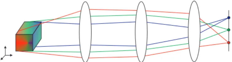
The SIR (Separable Internal Representation) method in [9] provides such objective func-tion based on the differences between classes. The network can be trained layer after layer using this objective function starting from the first hidden layer. Perfect categorization and production of correct signals can be accomplished for each layer [9][10]. These front layers are served, suitably, as the auto-kernel function. The auto-kernel will utilize the differences between classes to train the front layers, and it will not use the class label information in its training process. The idea is expressed in Figure 1.
Besides the front layer, the mechanism of rear layers which are near the output layer has also been identified [13]. The main mechanism is the labeling. The cooperation of the front and rear layers complete the supervised MLP. We will include a labeling sector that contains several layers after the auto-kernel. The outputs of the objective function for the labeling sector are the class labels. The nL-dimensional output vector of the auto-kernel function is converted to the class label, where the C(x) dimension is 1 and all the other dimensions are−1.
Figure 1. The idea of the implementation of neural lens
hidden layer does produce correct isolated signals, it will be served as the last front layer,L, and as the output of the kernel. We expect that the number of reduced representations of the last front layer will equal to the number of classes,YL
=T.
3. Learning algorithm for auto-kernel function
Figure 2 shows the auto-kernel function and the labeling sector. This function consists of layered neurons. For a pair of patterns in the same class, (xp,xq) ∈ V, the synapse weights of each layer are adjusted by using the energy function [10],
Eatt(xp,xq) = 1 2
y(p,m)−y(q,m)
2
, (1)
to reduce the distance between their output vectors,y(p,m)−y(q,m)
. However, for different classes,(xp,xq)∈U, the weights are adjusted by using the energy function,
Erep(xp,xq) = −1 2
y(p,m)−y(q,m)
2
, (2)
to increase the distance between their output vectors. The difference between classes is implic-itly used in two energies. Note that the value of the class label is not used in these two objective functions. The value of the labels will be applied only in the labeling sector. The magnitude of the energy functions (1) and (2) are0≤Eatt(xp,xq)≤2n
m and−2nm ≤Erep(xp,xq)≤0. The value of (1) converges toward zero from 2nm. The value of (2) comes close to −2nm from zero.
The network is constructed layer after layer, starting from L = 1. A new hidden layer is added, Lnew=Lold+ 1, wheneverLold layers cannot accomplish the isolation. All synapse weights of the trained layers are fixed during the training of that additional layer,m =Lold+1. The synaptic weight matrix which connects the output of the (m−1)th layer and the input of the mth layer, is denoted by Wm. The W1 connects the input layer and the first
hidden layer. Applying the gradient descent method to the added layer, the two energies can be reduced efficiently during the training stage. The successfully trained network is used as the auto-kernel function to map out the pattern,xp, in the output space,y(p,L).
Suppose there are two classes,C(x)∈ {1,2}. The training algorithm is as follows:
1. For the added layerWm (Wm fromW1toWL) 2. For limited epochs
3. Pick two patterns in the same class, xp1 and xp2, which satisfy the following
condition
(xp1
,xp2
) = arg max
{(xi,xj)∈V}
y(i,m)−y(j,m)
2
. (3)
Among all pairs of patterns in the same class, the two patterns(xp1,xp2)have the longest
distance in the output space of themth layer. 4. Find the pair of patterns,xq1
andxq2
in different classes, which satisfy
(xq1
,xq2
) = arg min
{(xi,xj)∈U}
y(i,m)−y(j,m)
2
. (4)
The pair of patterns (xq1,
xq2)
Figure 2. The auto-kernel function and labeling sector
5. Adjust the weightWmtoward the direction of negative gradient,
∇Wm ← ηatt
∂Eatt(xp1,xp1)
∂Wm
+ηrep∂E
rep(xq1,xq2)
∂Wm
(5)
Wm ← Wm− ∇Wm,
whereηattandηrepare learning rates.
The gradients ofEatt andErep in (5) are
∂Eatt(xp1,xp2)
∂Wm = (6)
+ (
y(p1,m)
1 −y (p2,m)
1
) (
1−y(p1,m)
1
) (
1 +y(p1,m)
1
) ..
. (
y(p1,m)
nm −y
(p2,m)
nm
) (
1−y(p1,m)
nm
) (
1 +y(p1,m)
nm ) [
y(p1,m−1)
1 , . . . , y(p
1,m−1)
nm−1 ,−1 ] − (
y(p1,m)
1 −y (p2,m)
1
) (
1−y(p2,m)
1
) (
1 +y(p2,m)
1
) ..
. (
y(p1,m)
nm −y
(p2,m)
nm
) (
1−y(p2,m)
nm
) (
1 +y(p2,m)
nm ) [
y(p2,m−1)
1 , . . . , y(p
2,m−1)
and
∂Erep(xq1,xq2)
∂Wm = (7)
− (
y(q1,m)
1 −y (q2,m)
1
) (
1−y(q1,m)
1
) (
1 +y(q1,m)
1
) ..
. (
y(q1,m)
nm −y
(q2,m)
nm
) (
1−y(q1,m)
nm
) (
1 +y(q1,m)
nm ) [
y(q1,m−1)
1 , . . . , y(q
1,m−1)
nm−1 ,−1 ] + (
y(q1,m)
1 −y (q2,m)
1
) (
1−y(q2,m)
1
) (
1 +y(q2,m)
1
) ..
. (
y(q1,m)
nm −y
(q2,m)
nm
) (
1−y(q2,m)
nm
) (
1 +y(q2,m)
nm ) [
y(q2,m−1)
1 , . . . , y(q
2,m−1)
nm−1 ,−1 ]
.
4. Experimental analysis
Two artificial datasets are used in the simulations. One is a two-class problem and the other is a three-class problem. Eight datasets collected from the real world are also used in the simulations.
4.1. Two-class problem
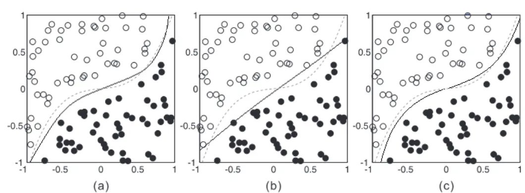
Figure 3(a) shows the result of the trained auto-kernel function for the two-class patterns, C(x)∈ {1,−1}, in the two-dimensional space,n0 = 2. The border of the two-class pattern is
the cubic equation,(x1)3+0.1x1 =x2.Points with the same color are of the same class. There
are five neurons in each layer, {nm = 5, m∈ {1, . . . , L}}. The kernel function is trained layer after layer until it produces correct isolated signals for each class. We set the isolation condition for inter-class representations as
min
{(xp,xq)∈U}
y(p,L)−y(q,L)
2
≈22×nL, (8)
and the condition for intra-class patterns as
max
{(xp,xq)∈V}
y(p,L)−y(q,L)
2
≈0. (9)
The learning rates are ηatt = 0.01 and ηrep = 0.1. The perfect isolation is reached when
L= 2. We set one neuron,nc
1 = 1,in the labeling sector as the output layer and use the class
identities, C(x) ∈ {1,−1}, to train this neuron. Figure 3(a) shows the result of the trained layers.
We also compare this result with those obtained by the traditional MLP [17] in Figure 3(b), and SVM in Figure 3(c). The traditional MLP with two hidden layers,nM LP
1 =nM LP2 = 5,is
trained by the supervised back-propagation. The polynomial kernel,K(u,v) =(
uTv+ 1)3 , is used in SVM [2].
4.2. Multiple-class problem
Figure 3. (a) The result of auto-kernel function. (b) The training result of traditional MLP. (c) The result of SVM.
nm = 9, nm = 11}. Each layer is trained with1000epochs. The isolation condition (9) is used in this simulation to stop the addition of any new layer. The learning rates areηatt = 0.01 andηrep = 0.1. The values of the isolations and conditions of each layer:
M inInterClass(m) = min
{(xp,xq)∈V}
y(p,m)−y(q,m)
2
(10)
and
M axIntraClass(m) = max
{(xp,xq)∈U}
y(p,m)−y(q,m)
2
, (11)
are recorded and plotted for the casenm = 5in Figure 4.
Figure 4. The curves record isolation conditions for the casenm = 5,M inInterClassin (10) and
M axIntraClassin (11), for each layer,m= 1,2,3,4.
When the perfect isolation is reached, we set two layers in the labeling sector withnc
1 = 2
andnc
2 = 3and use the class identities to train these additional two layers. In the layernc2 = 3,
each neuron represents a single class.
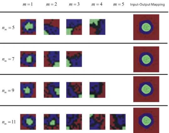
We employ the SOM (Self-Organizing Map) [6], which can visualize the nonlinear data, to visualize the output signals y(p,m) of each layer, and to see the isolation of classes. The neurons of the SOM are placed at regular points; see Figure 5. The SOM consists of10×10 neurons. Figure 6 shows the SOM result for all layers. Each node denotes a SOM neuron and is colored according to the label of its closest pattern. The output signals of the last layer have three concentrated points in the SOM.
4.3. Real dataset
Figure 5. The structure of the SOM used for the visualization of internal representations
Figure 6. The colored neurons in SOM visualize the isolation of the output vectors of each layer. The images on the most right column display the mapping relation between input space and output space.
The iris dataset [5] contains 150 patterns items which belong to four classes. Each pattern is a four dimensional vector. The Wisconsin breast cancer database is a diagnostic dataset. Many useful attributes are used for the prediction of benign or malignant tumors, a two-class problem. The study in [20] reported a95.9%testing accuracy. This breast cancer dataset has 16missing values. These missing values are set to zero. The Parkinson dataset [14] contains the biomedical voice measurement given by healthy people and Parkinson patients.
Four machine learning techniques, k-NN (k-nearest neighbors algorithm), auto-kernel function, traditional MLP and SVM, are compared using the 10-fold cross-validation. The dataset is randomly split into ten partitions, nine of them are used in the training process and the one at rest is used in the testing process. The result is the average of the 10-fold cross-validation. The labeling sector for the iris set arenc
cancer dataset are nc
1 = 5 andnc2 = 1.The sector for the Parkinson dataset are nc1 = 5 and
nc
2 = 3.The settings of the labeling sector for all datasets are listed in Table 1. The
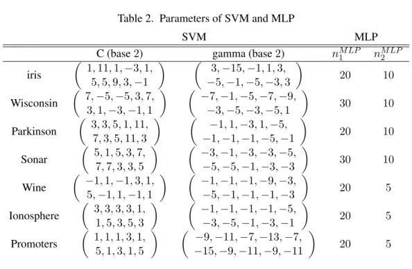
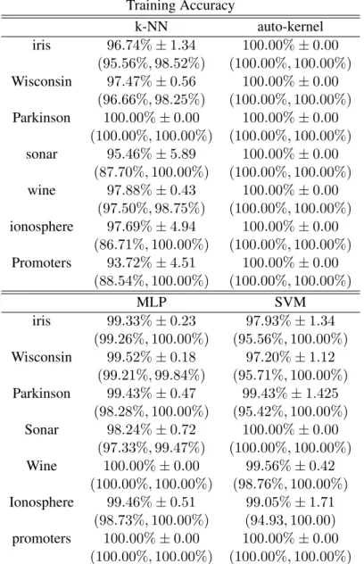
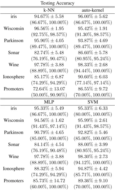
parame-ters of SVM are the cost C for the error tolerance and the gammaγ in the Gaussian kernel. Parameterk indicates the number of neighboring cells in the k-NN algorithm. The values of C, γ, and k, are optimized using an inner 10-fold cross-validation procedure. The settings that produce the lowest errors are used to train the models on all of the training patterns. The traditional MLP has two hidden layers. All parameters are listed in Table 1 and Table 2. The values of the input patterns are normalized to the range[−1,1]. Table 3 and Table 4 record the training and testing accuracy, and show the standard deviation. Both of them are the average among ten-fold examinations. The two percentages in brackets under the average accuracy indicate the minimal and maximal testing accuracy of 10-fold cross-validation. The 100% accuracy of training is not considered over-fitting because the prediction accuracy does not decline when the training accuracy increases.
Table 1. Parameters of k-NN and auto-kernel function
k-NN auto-kernel
k (nm, nc1, nc2)
iris (1,1,1,1,1,1,1,1,1,1) (11,5,3)
Wisconsin (3,7,5,13,9,5,7,13,3,5) (30,10,1)
Parkinson (1,1,1,1,1,1,1,1,1,1) (20,20,1)
sonar (3,1,1,3,3,3,1,1,1,1) (35,5,1)
wine (3,15,13,11,19,15,19,13,15,11) (10,5,3)
ionosphere (1,3,1,1,1,1,11,1,1,1) (10,5,1)
promoters (3,5,1,3,1,3,3,3,3,3) (100,40,1)
Table 2. Parameters of SVM and MLP
SVM MLP
C (base2) gamma (base2) nM LP1 nM LP2
iris
(
1,11,1,−3,1,
5,5,9,3,−1
) (
3,−15,−1,1,3,
−5,−1,−5,−3,3
)
20 10
Wisconsin
(
7,−5,−5,3,7,
3,1,−3,−1,1
) (
−7,−1,−5,−7,−9,
−3,−5,−3,−5,1
)
30 10
Parkinson
(
3,3,5,1,11,
7,3,5,11,3
) (
−1,1,−3,1,−5,
−1,−1,−1,−5,−1
)
20 10
Sonar
(
5,1,5,3,7,
7,7,3,3,5
) (
−3,−1,−3,−3,−5,
−5,−5,−1,−3,−3
)
30 10
Wine
(
−1,1,−1,3,1,
5,−1,1,−1,1
) (
−1,−1,−1,−9,−3,
−5,−1,−1,−1,−3
)
20 5
Ionosphere
(
3,3,3,3,1,
1,5,3,5,3
) (
−1,−1,−1,−1,−5,
−3,−5,−1,−3,−1
)
20 5
Promoters
(
1,1,1,3,1,
5,1,3,1,5
) (
−9,−11,−7,−13,−7,
−15,−9,−11,−9,−11
)
20 5
5. Conclusion
Table 3. The training accuracy on real dataset
Training Accuracy
k-NN auto-kernel iris 96.74%±1.34 100.00%±0.00
(95.56%,98.52%) (100.00%,100.00%)
Wisconsin 97.47%±0.56 100.00%±0.00 (96.66%,98.25%) (100.00%,100.00%)
Parkinson 100.00%±0.00 100.00%±0.00 (100.00%,100.00%) (100.00%,100.00%)
sonar 95.46%±5.89 100.00%±0.00 (87.70%,100.00%) (100.00%,100.00%)
wine 97.88%±0.43 100.00%±0.00 (97.50%,98.75%) (100.00%,100.00%)
ionosphere 97.69%±4.94 100.00%±0.00 (86.71%,100.00%) (100.00%,100.00%)
Promoters 93.72%±4.51 100.00%±0.00 (88.54%,100.00%) (100.00%,100.00%)
MLP SVM
iris 99.33%±0.23 97.93%±1.34 (99.26%,100.00%) (95.56%,100.00%)
Wisconsin 99.52%±0.18 97.20%±1.12 (99.21%,99.84%) (95.71%,100.00%)
Parkinson 99.43%±0.47 99.43%±1.425 (98.28%,100.00%) (95.42%,100.00%)
Sonar 98.24%±0.72 100.00%±0.00 (97.33%,99.47%) (100.00%,100.00%)
Wine 100.00%±0.00 99.56%±0.42 (100.00%,100.00%) (98.76%,100.00%)
Ionosphere 99.46%±0.51 99.05%±1.71 (98.73%,100.00%) (94.93,100.00)
promoters 100.00%±0.00 100.00%±0.00 (100.00%,100.00%) (100.00%,100.00%)
SVM is also close to the intrinsic border. However, the SVM has learned a similar boundary to the traditional MLP in Figure 3(b) while using the Gaussian kernel. The SOM result for all layers shows that well isolated signals are gradually accomplished in the last few layers. The last result shows that the auto-kernel function is competitive and practical in real world applications.
Acknowledgement
This work was supported by National Science Council under the project NSC101-2811-M-001-082.
References
Table 4. The testing accuracy on real dataset
Testing Accuracy
k-NN auto-kernel iris 94.67%±5.58 96.00%±5.62
(86.67%,100.00%) (86.67%,100.00%)
Wisconsin 96.56%±1.95 95.42%±1.91 (92.75%,98.57%) (91.30%,98.57%)
Parkinson 95.90%±4.05 93.87%±4.69 (89.47%,100.00%) (89.47%,100.00%)
Sonar 82.74%±5.48 86.60%±5.78 (76.19%,90.47%) (80.95%,95.24%)
Wine 97.78%±3.88 98.33%±2.68 (88.89%,100.00%) (94.44%,100.00%)
Ionosphere 85.17%±6.87 90.60%±6.03 (74.29%,94.29%) (77.14%,97.14%)
Promoters 72.64%±13.07 86.55%±9.72 (50.00%,90.90%) (70.00%,100.00%)
MLP SVM
iris 95.33%±5.49 95.33%±6.33 (86.67%,100.00%) (80.00%,100.00%)
Wisconsin 94.56%±1.62 95.99%±2.61 (91.43%,97.14%) (91.43%,98.57%)
Parkinson 90.79%±4.65 92.82%±5.46 (85.00%,100.00%) (85.00%,100.00%)
Sonar 84.14%±4.54 88.00%±3.99 (76.19%,90.48%) (80.95%,95.24%)
Wine 97.78%±3.88 98.30%±2.73 (88.89%,100.00%) (94.12%,100.00%)
Ionosphere 88.32%±5.94 94.87%±4.42 (74.29%,94.29%) (85.71%,100.00%)
Promoters 85.73%±14.72 89.36%±9.10 (60.00%,100.00%) (70.00%,100.00%)
[2] C.-C. Chang and C.-J. Lin. Libsvm : a library for support vector machines. Software available at http://www.csie.ntu.edu.tw/ cjlin/libsvm, 2001.
[3] W.-C. Cheng and C.-Y. Liou. Manifold construction using the multilayer perceptron. InLecture Notes In Computer Science, volume 5163, Part I, pages 119–127, 2008.
[4] W.-C. Cheng and C.-Y. Liou. Linear replicator in kernel space. Lecture Notes in Computer Science, 6064, Part II:75–82, 2010.
[5] R.A. Fisher. The use of multiple measurements in taxonomic problems. Annals of Eugenics, 7 Part II:179–188, 1936.
[6] T. Kohonen. Self-organized formation of topologically correct feature maps. Biological Cyber-netics, 43:59–69, 1982.
[7] O. Krejcar, D. Janckulik, and L. Motalova. Complex biomedical system with biotelemetric monitoring of life functions. InProceedings of the IEEE Eurocon, pages 138–141, 2009. [8] O. Krejcar, D. Janckulik, and L. Motalova. Complex biomedical system with mobile clients. In
[9] C.-Y. Liou, H.-T. Chen, and J.-C. Huang. Separation of internal representations of the hidden layer. InProceedings of the 2000 International Computer Symposium, pages 26–34, 2000. [10] C.-Y. Liou and W.-C. Cheng. Resolving hidden representations. InLecture Notes in Computer
Science, volume 4985, Part II, pages 254–263. Springer, Heidelberg, 2008.
[11] C.-Y. Liou and W.-C. Cheng. Forced accretion and assimilation based on self-organizing neural network. InSelf Organizing Maps - Applications and Novel Algorithm Design, pages 683–702, 2011.
[12] C.-Y. Liou and W.-J. Yu. Initializing the weights in multilayer network with quadratic sigmoid function. In Proceedings of the International Conference on Neural Information Processing, pages 1387–1392, 1994.
[13] C.-Y. Liou and W.-J. Yu. Ambiguous binary representation in multilayer neural network. In Proceedings of International Conference on Neural Networks, volume 1, pages 379–384, 1995. [14] M.A. Little, P.E. McSharry, S.J. Roberts, D.A.E. Costello, and I.M. Moroz. Exploiting nonlinear
recurrence and fractal scaling properties for voice disorder detection. BioMedical Engineering OnLine, 6:23, 2007.
[15] J. Mercer. Functions of positive and negative type and their connection with the theory of integral equations. Philosophical Transactions of the Royal Society A, 209:415V446, 1909.
[16] L. Pearson. On lines and planes of closest fit to systems of points in space. Philosophical Magazine, 2(11):559–572, 1901.
[17] D.E. Rumelhart, G.E. Hinton, and R.J. Williams. Learning internal representations by error propagation. InParallel Distributed Processing: Explorations in the Microstructure of Cogni-tion, volume 1, pages 318–362. Cambridge, MA: MIT Press, 1986.
[18] Bernhard Scholkopf, Alexander Smola, and Klaus-Robert Muller. Nonlinear component analysis as a kernel eigenvalue problem. Psychometrika, 10:1299–1319, 1998.
[19] Vladimir Vapnik. The nature of statistical learning theory. InInformation Science and Statistics, 2000.