Earth Syst. Sci. Data, 2, 261–273, 2010 www.earth-syst-sci-data.net/2/261/2010/ doi:10.5194/essd-2-261-2010
©Author(s) 2010. CC Attribution 3.0 License. Open
Access
Earth System
Science
Data
A consistent data set of Antarctic ice sheet topography,
cavity geometry, and global bathymetry
R. Timmermann1, A. Le Brocq2, T. Deen3, E. Domack4, P. Dutrieux3, B. Galton-Fenzi5, H. Hellmer1, A. Humbert6, D. Jansen7, A. Jenkins3, A. Lambrecht8, K. Makinson3, F. Niederjasper1, F. Nitsche9,
O. A. Nøst10, L. H. Smedsrud11, and W. H. F. Smith12
1Alfred Wegener Institute for Polar and Marine Research, Bremerhaven, Germany
2University of Exeter, Exter, UK
3British Antarctic Survey, Cambridge, UK
4Hamilton College, Clinton, NY, USA
5University of Tasmania, Hobart, Tasmania
6KlimaCampus, University of Hamburg, Hamburg, Germany
7Swansea University, Swansea, UK
8University Innsbruck, Innsbruck, Austria
9Lamont-Doherty Earth Observatory, Columbia University, Palisades, NY, USA
10Norwegian Polar Institute, Tromsø, Norway
11Bjerknes Centre for Climate Research, Bergen, Norway
12Laboratory for Satellite Altimetry, NOAA NESDIS, Silver Spring, MD, USA
Received: 21 July 2010 – Published in Earth Syst. Sci. Data Discuss.: 29 July 2010 Revised: 4 November 2010 – Accepted: 13 November 2010 – Published: 22 December 2010
Abstract. Sub-ice shelf circulation and freezing/melting rates in ocean general circulation models depend critically on an accurate and consistent representation of cavity geometry. Existing global or pan-Antarctic topography data sets have turned out to contain various inconsistencies and inaccuracies. The goal of this work is to compile independent regional surveys and maps into a global data set. We use the S-2004 global 1-min bathymetry as the backbone and add an improved version of the BEDMAP topography (ALBMAP bedrock topography) for an area that roughly coincides with the Antarctic continental shelf. The position
of the merging line is individually chosen in different sectors in order to capture the best of both data sets.
High-resolution gridded data for ice shelf topography and cavity geometry of the Amery, Fimbul, Filchner-Ronne, Larsen C and George VI Ice Shelves, and for Pine Island Glacier are carefully merged into the ambient ice and ocean topographies. Multibeam survey data for bathymetry in the former Larsen B cavity and the southeastern Bellingshausen Sea have been obtained from the data centers of Alfred Wegener Institute (AWI), British Antarctic Survey (BAS) and Lamont-Doherty Earth Observatory (LDEO), gridded, and blended into the existing bathymetry map. The resulting global 1-min Refined Topography data set (RTopo-1) contains self-consistent maps for upper and lower ice surface heights, bedrock topography, and surface type (open ocean, grounded ice, floating ice, bare land surface). The data set is available in NetCDF format from the PANGAEA
database at doi:10.1594/pangaea.741917.
Correspondence to:R. Timmermann
1 Introduction
Heat and salt fluxes at the base of any ice shelf, the properties of water masses within the cavity, and the exchange with the open ocean in numerical simulations strongly depend on an accurate and consistent representation of ice-shelf draft and sub-ice bathymetry. Early attempts to quantify the contribu-tion of Ice Shelf Water to the Southern Ocean’s hydrogra-phy (e.g. Hellmer and Jacobs, 1995; Beckmann et al., 1999; Timmermann et al., 2001; Assmann et al., 2003) had to ad-mit significant uncertainties due to partly crude assumptions about the geometry of ice shelf cavities. Local or regional simulations of individual cavities and the adjacent seas were
able to use more detailed data sets but suffered from
uncer-tainties arising from the choice of open or closed boundary conditions (e.g. Gerdes et al., 1999; Grosfeld et al., 2001; Williams et al., 2001; Thoma et al., 2006; Dinniman et al., 2007) and had no possibility to investigate larger-scale im-pacts and feedbacks.
Melting of glaciers, ice caps and ice sheets contributes to changes of the global sea level. Therefore, an estimate of the rate of ice mass loss from the Antarctic ice sheet is an im-portant component in the IPCC’s Fifth Assessment Report. Given that most of the Antarctic ice sheet drains into float-ing glaciers or ice shelves, model estimates of sub-ice shelf melting rates are crucial to obtain a reliable estimate of the southern hemisphere’s ice mass budget. In order to reduce uncertainties for high-resolution simulations of the coupled ocean-sea ice-ice shelf system in circumpolar or global ocean general circulation models, we compiled consistent maps
for Antarctic ice sheet/shelf topography and global ocean
bathymetry. These maps combine available gridded data with independent high-resolution data sets and original multibeam echosounder surveys. To preserve as much as possible infor-mation from the source data sets and to ensure an easy inter-polation to any model grid, we chose a resolution of 1 min in zonal and meridional direction, although we are aware that large parts of the available information in high latitudes is less detailed than this grid spacing might suggest.
In this paper, we present the data sets used, discuss their spatial coverage and the preprocessing applied, the strategies followed for merging data sets, and the resulting maps of ice and bedrock topography. In contrast to the activities towards an International Bathymetric Chart of the Southern Ocean (IBCSO) (e.g., Schenke and Ott, 2009), our main goal is not
a remapping of bathymetric data in the region south of 50◦S,
but a consistent representation of Antarctic ice sheet/shelf
to-pography and global bathymetry in a data set that contains enough detail for a wide range of regional and larger-scale studies. The main target group includes, but is not restricted to ocean modellers who aim at a realistic representation of Southern Ocean ice shelf processes in ocean general circula-tion models.
2 Data sets and processing
2.1 Overview
The RTopo-1 data set (see Figs. 1 and 2 for an overview) comprises global 1-min fields for
– bedrock topography (ocean bathymetry; surface
topog-raphy of continents; bedrock topogtopog-raphy under ice
sheets/shelves)
– surface elevation (upper ice surface height for Antarctic
ice sheet/shelves; bedrock elevation for ice-free
conti-nent; zero for ocean)
– ice base topography for the Antarctic ice sheet/ice shelf
system (ice draft for ice shelves; zero in the absence of ice)
– masks to identify open ocean, ice sheet, ice shelf, and
bare land surface
– locations of coast and grounding lines (consistent with
mask) for easy plotting
For ice-free land surface, thebedrock topographyandsurface
elevationmaps are identical. Naturally,bedrock topography
andice base topographyare equal for grounded ice. Ice not
connected to the Antarctic ice sheet, including glaciers on subantarctic islands and the Greenland ice sheet, is not cov-ered in our data set; these areas are labeled as bare land sur-face with the sursur-face elevation preserved.
Note that in the following we use the term “ice shelf to-pography” for a consistent combination of ice top and bottom surface heights. The term “cavity geometry” refers to a com-pilation of ice-shelf draft and sub-ice (cavity) bathymetry.
2.2 Data sources
2.2.1 World Ocean bathymetry
The nucleus of RTopo-1 is the S-2004 1-minute digital ter-rain model (Marks and Smith, 2006), which is a combina-tion of the gravimetry-based Smith and Sandwell (1997) map with the General Bathymetric Chart of the Oceans (GEBCO) One Minute Grid. GEBCO has been interpolated from dig-itized contours derived from ship-based echo-soundings and is therefore artificially smooth in many places. The two prod-ucts were combined using GEBCO at locations poleward of
72◦latitude or shallower than 200 m depth (and on land), and
Smith and Sandwell (1997) equatorward of 70◦ and deeper
R. Timmermann et al.: Antarctic ice sheet topography, cavity geometry, and global bathymetry 263
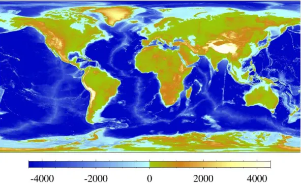
Figure 1. RTopo-1 global bedrock topography. On continents outside Antarctica, this represents the topography of the solid surface (including bottom of lakes, surface elevation of glaciers and continental ice caps) and mirrors the S-2004 data set.
For the continental shelf regions of the Southern Ocean, however, where satellite gravity data are not available, many uncertainties remain. Ice shelves are not represented in S-2004 at all; instead they appear as areas with zero surface height. For the Antarctic continent, S-2004 contains the (ice) surface elevation, but not the bedrock topography.
We therefore use the S-2004 digital terrain model as the global backbone bathymetry outside the immediate vicinity of Antarctica. We keep lakes and other features with a sur-face height below mean sea level and no connection to the world ocean, but mark them as continent in the surface type mask (see Sect. 2.3). Antarctica and most of the Antarctic continental shelf are covered by a suite of regional and lo-cal data sets (Fig. 3), which are discussed in the following sections.
2.2.2 Antarctic ice and bedrock topographies
Upper and lower surface elevations for the Antarctic ice sheet and some of the ice shelves (see below for those not included) and ocean bathymetry for most of the Antarctic continen-tal shelf are based on an improved version of the BEDMAP data set that will be refered to as ALBMAP hereafter. With
the BEDMAP effort (Lythe et al., 2001), original survey data
collected over about 50 years were compiled into seamless digital topography models for the Antarctic continent and ice sheet. For ALBMAP, Le Brocq et al. (2010) incorpo-rated several new data sets. Ice surface elevation for most of Antarctica has been derived from the 1 km digital eleva-tion model (DEM) of Bamber et al. (2009). For the
Antarc-tic Peninsula, the RAMP DEM (Liu et al., 1999) has been added. An improved representation of sub-ice shelf cavi-ties has been achieved by using spline-based interpolation. Bedrock depth in ALBMAP has been carefully corrected (mostly increased) towards the grounding line for many ice shelves. Maybe most important, ALBMAP ensures
consis-tency of the different maps along the grounding lines and
in-troduces a surface type mask for grounded ice, floating ice, and open water.
Like BEDMAP, ALBMAP uses a stereographic projec-tion, which is very convenient for studies of the Antarctic
ice sheet/shelf system, but much less so for circumpolar or
global ocean models. We use spherical Delauney triangula-tion as a basis for linear interpolatriangula-tion to our regular 1-min (lon, lat) grid.
To ensure a smooth continuation of bathymetry into the sub-ice shelf cavities, we merge the ALBMAP data into S-2004 not strictly along the ice-shelf edge, but at a line that has been carefully adjusted to capture the best from both data sets (Fig. 3). In the East Antarctic and many other places, the transition line follows the ice shelf front or the coast line. In order to avoid the spurious signature of General Belgrano Bank, which has been reported to be only a minor rise (with an elevation of only 20 m above the surrounding flat bottom) by Nicholls et al. (2003), we use ALBMAP for the entire continental shelf in the southwestern Weddell Sea
south of 66.15◦S with the transition occuring between the
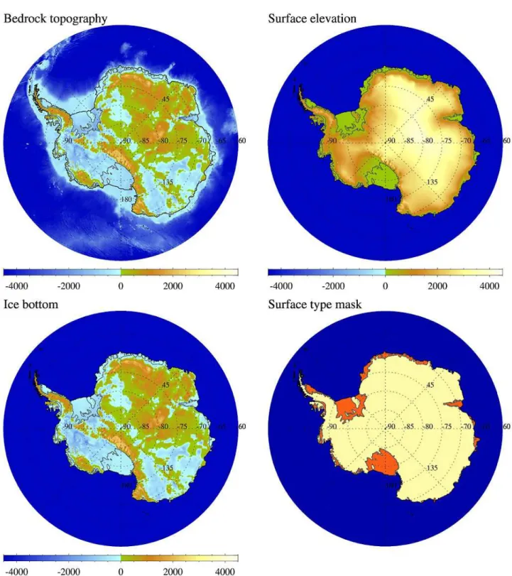
Figure 2.Antarctic subset of the RTopo-1 data set. Top left: Bedrock topography (ocean bathymetry). Top right: surface elevation. Bottom left: ice bottom surface height (including ice shelf draft). Bottom right: surface type mask, blue=ocean, yellow=grounded ice, orange=
R. Timmermann et al.: Antarctic ice sheet topography, cavity geometry, and global bathymetry 265
Figure 3.Data sources for ocean bathymetry (left) and ice sheet/shelf topography (right). See Table 1 for an explanation of numbers. Grey areas mark transition zones between the data sets.
and 4000 m water depth. Tangens hyperbolicus functions are used to ensure a smooth transition between the data sets with-out too much spurious blurring of gradients. The width of the transition corridor varies and can be seen in the left panel of Fig. 3.
In order to incorporate topographic information from sur-veys that have been conducted after the BEDMAP data set had been published, we replace ice and ocean topographies by newer, regional data sets in several places outlined in the following sections (Table 1). Again we use spherical trian-gulation as a basis for interpolation and tangens hyperbolicus functions of the ratio between “new” and “background” data
in a data window of typically 1◦width for the transition
be-tween data sets. Wherever interpolation artefacts lead to in-consistencies between ice shelf draft and ocean bathymetry (resulting in negative water column thickness), we apply a minimum water column thickness of 10 m.
2.2.3 Filchner-Ronne Ice Shelf
Upper and lower surface heights for Filchner-Ronne Ice Shelf and the position of the ice shelf front are derived from the ice thickness data sets of Lambrecht et al. (2007) using their Eq. (2) with the proposed densities and parameter val-ues. Given their small-scale and transient nature, the inlets downstream from Hemmen Ice Rise are filled with interpo-lated values.
Bathymetry in the Filchner-Ronne Ice Shelf cavity is de-rived from the data set compiled by Makinson and Nicholls (1999). In order to maintain floating ice in the embayment with the inflow of Support Force Glacier, we deviate from the ALBMAP grounding line here and apply the grounding line position of Rignot and Jacobs (2002) instead, which is consistent with the maps of Makinson and Nicholls (1999) and Lambrecht et al. (2007) at this location. The ice plain to the west and the ice rumples east of Bungenstockr¨ucken (Heidrich et al., 1992; Scambos et al., 2004) are treated as grounded ice.
Inconsistencies between the two data sets (ice thickness and bathymetry) are addressed by applying a minimum wa-ter column thickness of 10 m in the area of floating ice and enforcing zero water column thickness in locations with grounded ice. Given the high accuracy of the ice shelf thick-ness estimates (error quantified to be less than 25 m by the authors), we retain the Lambrecht et al. (2007) draft field and apply the corrections to the bathymetry; they are typi-cally between 100 and 200 m and occur localized in a narrow band along the grounding line.
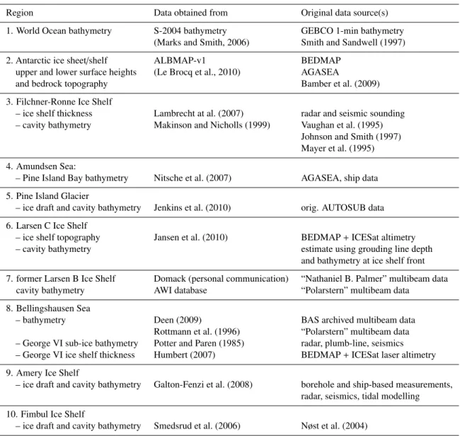
Table 1.Data sources for individual regions of the Southern Ocean, as merged into RTopo-1. Numbers in the Region column correspond to the source flag in Fig. 3
Region Data obtained from Original data source(s)
1. World Ocean bathymetry S-2004 bathymetry GEBCO 1-min bathymetry
(Marks and Smith, 2006) Smith and Sandwell (1997)
2. Antarctic ice sheet/shelf ALBMAP-v1 BEDMAP
upper and lower surface heights (Le Brocq et al., 2010) AGASEA
and bedrock topography Bamber et al. (2009)
3. Filchner-Ronne Ice Shelf
– ice shelf thickness Lambrecht at al. (2007) radar and seismic sounding
– cavity bathymetry Makinson and Nicholls (1999) Vaughan et al. (1995)
Johnson and Smith (1997) Mayer et al. (1995)
4. Amundsen Sea:
– Pine Island Bay bathymetry Nitsche et al. (2007) AGASEA, ship data
5. Pine Island Glacier
– ice draft and cavity bathymetry Jenkins et al. (2010) orig. AUTOSUB data
6. Larsen C Ice Shelf
– ice shelf topography Jansen et al. (2010) BEDMAP+ICESat altimetry
– cavity bathymetry estimate using grouding line depth
and bathymetry at ice shelf front
7. former Larsen B Ice Shelf Domack (personal communication) “Nathaniel B. Palmer” multibeam data
cavity bathymetry AWI database “Polarstern” multibeam data
8. Bellingshausen Sea
– bathymetry Deen (2009) BAS archived multibeam data
Rottmann et al. (1996) “Polarstern” multibeam data
– George VI sub-ice bathymetry Potter and Paren (1985) radar, plumb-line, seismics
– George VI ice shelf thickness Humbert (2007) BEDMAP+ICESat laser altimetry
9. Amery Ice Shelf
– ice draft and cavity bathymetry Galton-Fenzi et al. (2008) borehole and ship-based measurements, radar, seismics, tidal modelling
10. Fimbul Ice Shelf
– ice draft and cavity bathymetry Smedsrud et al. (2006) Nøst et al. (2004)
Open ocean bottom topography in Pine Island Bay, how-ever, utilizes the data set from Nitsche et al. (2007), which is a combination of ship data with the “Airborne Geophys-ical Survey of the Amundsen Embayment” (AGASEA) and BEDMAP data sets. This data set has already been included in ALBMAP, but to preserve its fine resolution we use the original Nitsche et al. (2007) data here.
For upper and lower ice surface height and cavity bathymetry for most ice shelves in the Amundsen Sea we retain the data from ALBMAP, which in turn uses AGASEA data (Vaughan et al., 2006; Holt et al., 2006) for Thwaites Glacier Tongue, and Crosson and Dotson Ice Shelves.
An important exception is Pine Island Glacier (PIG), where the geometry of the sub-ice cavern (ice-shelf draft and sub-ice bathymetry) is interpolated from the very recent
AUTOSUB data of Jenkins et al. (2010). While BEDMAP and S-2004 do not contain any meaningful information for the sub-PIG cavity, the AUTOSUB survey revealed a trough with a depth of more than 1000 m at the ice front and a sill of about 300 m height located halfway between glacier front and grounding line (see Fig. 6 below). Water column thickness in the cavity thus varies from about 700 m near the glacier front to only 275 m at the sill, but then again increases to a maximum of 360 m towards the grounding line.
2.2.5 Larsen C Ice Shelf
R. Timmermann et al.: Antarctic ice sheet topography, cavity geometry, and global bathymetry 267
Figure 4. Surface elevation (left) and ice shelf draft (right) for the Antarctic Peninsula, including Larsen C ice shelf and the remnants of Larsen B ice shelf. The ice shelf front is marked with a black line, the grounding line location with a grey line. The letters A/B/C mark the (former) Larsen A, B and C Ice Shelves.
heights obtained from ICESat altimetry. The grounding line location in this data set has been picked from
interferome-try from the ERS-1/ERS-2 tandem mission in the north and
from MODIS imagery in the south. It is a rather conserva-tive estimate in a sense that for all areas denoted as ice shelf
we can be sure to find floating ice in reality. Differences from
BEDMAP draft occur mainly along the ice shelf front, where the ice is thinner now, and towards the grounding line, where the depth of the ice shelf base increases to about 550 m below sea level (Fig. 4).
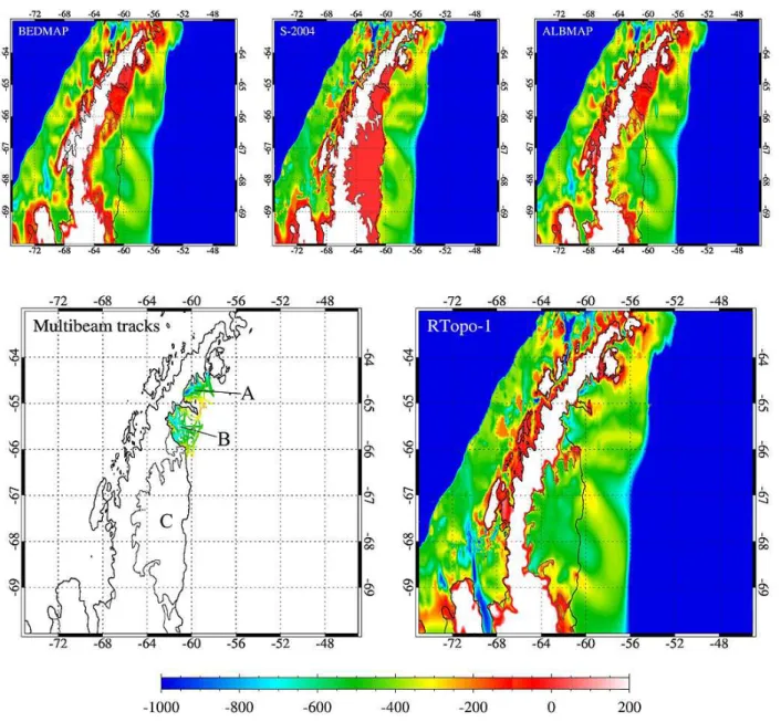
Bottom topography in the cavity below Larsen C Ice Shelf is based on ALBMAP, but it has been modified in order to ensure a minumum water column thickness of 10 m near the grounding line and a gradual rise to the bottom depth found near the ice shelf front. Bathymetry now features a depth be-tween 500 and 600 m under most of the ice shelf with deep troughs towards the grounding line (Fig. 5). The existence of such deep troughs in immediate vicinity to the mountains of the Antarctic Peninsula might seem doubtable at first glance; multibeam bathymetry surveys in Antarctic Sound and the former Larsen B Ice Shelf cavity (Gavahan and Domack, 2006), however, show that in fact troughs of very similar depth and horizontal scale have been carved out where ice streams eroded the ocean bottom. In any case it should be kept in mind that bathymetry in the Larsen C Ice Shelf cavity in our data set is hardly more than an educated guess.
2.2.6 Larsen A and B Ice Shelves
The disintegration of Larsen A and B Ice Shelves in Jan-uary 1995 and FebrJan-uary 2002, respectively, transformed the former cavities into open water embayments. For the
bathymetry in this area, we combine original data from
“Po-larstern” cruise ANT-XXIII/8 (Pugacheva and Lott, 2008)
with digitized maps of along-track multibeam data from the “Nathaniel B. Palmer” NBP0107 and NBP0603 cruise re-ports (E. Domack, personal communication, 2009). Again spherical triangulation is used to fill the gaps between cruise tracks (Fig. 5). The coastline of the Larsen B embayment has been corrected wherever the existence of ship tracks suggests the presence of open water instead of ice or continent.
2.2.7 Bellingshausen Sea and George VI Ice Shelf For the eastern Bellingshausen Sea shelf area (i.e. the area
shallower than 1000 m in the sector east of 90◦W and south
of 67◦S), bathymetry in our data set is mainly based on
multibeam swath data from the BAS bathymetry database (Deen, 2009). Many of these data go back to “James Clark Ross” cruises JR104 and JR165 and have already been
fea-tured in the papers of ´O Cofaigh et al. (2005), Holland
et al. (2010), and Padman et al. (2010). We add original
data from R/VPolarsterncruise ANT-XI/3 (Rottmann et al.,
Figure 5. Different representations of bathymetry (bedrock topography) in the area of the Larsen Ice Shelves. Top row: BEDMAP (left), S-2004 (middle), and ALBMAP (right). Bottom row: Multibeam track data (left), and the RTopo-1 product (right). Ice shelf front and coastline are marked with a black line, grounding line location with a grey line. The letters A/B/C mark the (former) Larsen A, B and C Ice Shelf cavities.
channels provide connections to the continental shelf break. Note that we had to make assumptions for bathymetry in the data gap in the northern part of George VI Sound, but these are fully consistent with the Potter and Paren (1985) plumb line profile along the northern ice shelf front.
Surface elevation and draft of George VI Ice Shelf is de-rived from the Humbert (2007) thickness data set. Given that melt ponds occupy large parts of George VI Ice Shelf and that a distinguished firn layer is virtually absent, we convert
thickness to draft assuming an ice density of 910 kg m−3and
do not apply any firn correction.
2.2.8 Amery Ice Shelf
For Amery Ice Shelf and the Prydz Bay region, we use the ice draft and ocean bathymetry data of Galton-Fenzi et al. (2008), who combine radar and seismic surveys, ice thick-ness estimates from satellite altimetry, borehole and ship-based observations, and insight obtained from tidal mod-elling. This data set is substantially improved over BEDMAP and ALBMAP and features a much deeper ice draft
(maxi-mum≈2500 m) and bathymetry (maximum bottom depth in
the cavity ≈3000 m). It also introduces five grounded-ice
R. Timmermann et al.: Antarctic ice sheet topography, cavity geometry, and global bathymetry 269
Figure 6. Different representations of bathymetry (bedrock topography) in the Bellingshausen Sea. Top row: BEDMAP (left), S-2004 (middle), and ALBMAP (right). Bottom row: Multibeam track data (left), and the RTopo-1 product (right). Note the differences for Pine Island Glacier (PIG) and George VI sub-ice bathymetries. Black line represents the coastline or ice shelf front, dark grey line the grounding line.
2.2.9 Fimbul Ice Shelf
For Fimbul Ice Shelf draft and sub-ice bathymetry we use the topography data set of the regional model of Smedsrud et al. (2006), who interpolated original seismic data from Nøst (2004) covering the central and outer parts of the ice shelf. For the deeper parts of the cavity towards the ground-ing line where no seismic data are available, ice shelf draft and bathymetry were interpolated along the flow line of the Jutulstraumen ice stream. This interpolation leads to a chan-nel connecting the 1100 m deep Jutul basin with the deepest grounding line at the Fimbul ice shelf at 875 m depth.
We have retained the ALBMAP grounding line location here. Ice extent has been carefully reduced to match the more recent data.
Figure 7. Global surface type mask in RTopo-1. Blue=ocean, white=grounded ice, orange=ice shelf, grey=bare land surface.
line locations in the newly integrated local data sets are applied to Filchner-Ronne Ice Shelf (ice front; grounding line in the Support Force Glacier region), George VI Ice Shelf (ice front location in Ronne Entrance), Larsen C ice shelf (ice front and grounding line), Amery Ice Shelf (ice front, grounding line, ice rumples), and Fimbul Ice Shelf (ice front). Ice caps not connected to the Antarctic ice sheet (which at the resolution of the ALBMAP data set exist on the islands close to the Antarctic Peninsula, but not on the mainland of Antarctica) have been removed from the mask and are now classified as bedrock. Ice surface height in these cases has been adopted as the bedrock surface height. Sub-glacial lakes are ignored; bedrock elevation is assumed to be identical to the ice bottom surface height here.
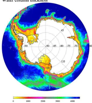
While lakes and enclosed seas outside Antarctica are still present in the bathymetry data set (adopted from S-2004), they are marked as “bare ground” in the mask. Using the to-pography map(s) together with the mask thus allows for an easy generation of global or regional ocean model grids with-out the need to manually remove features with a topography below mean sea level and no connection to the world ocean. Water column thickness (Fig. 8), which is needed, e.g., for the generation of ocean model grids with a terrain-following
vertical coordinate, can be computed as the difference
be-tween ice bottom surface height (which contains the ice draft for ice shelves and is zero in the open ocean) and ocean bedrock topography (bathymetry). Locations of nonzero en-tries in the resulting field are consistent with the area denoted as “ocean” in the mask.
Last but not least, the data set contains position data for coast and grounding lines that are consistent with the mask and all other (data) fields. These can be used for an easy and overlap-free plotting of maps in any desired projection (and have been used for all the maps in this paper).
2.4 Error estimates
For a synthesis of several data sets of very different nature,
errors are hard to quantify. This is partiularly true where val-ues have been inferred from consistency arguments, e.g. near
Figure 8.Water column thickness in the Southern Ocean sector of RTopo-1.
the coast or grounding lines and in the transition corridors
be-tween different data sets. Here we give an overview on error
estimates provided by the authors of some of our source data sets.
2.4.1 Ice surface height
Griggs and Bamber (2009) used airborne altimeter data from four campaigns in Antarctica covering a wide range of sur-face slopes and ice sheet regions to assess the accuracy of the Bamber et al. (2009) 1-km DEM. They found that
root-mean-squared differences varied from about 5 m in a region
with gentle slopes near Ross Ice Shelf to about 35 m at the Antarctic Peninsula where surface slopes are steep and the across-track spacing of the satellite data is relatively large. Errors ranged from typically 1 m over the ice shelves to 2– 6 m for the majority of the grounded ice sheet. In the steeply sloping margins along the Peninsula and mountain ranges the error was estimated to be several tens of metres. Given that this data set is one of the backbone data sets in ALBMAP, these numbers indicate a likely range for surface elevation errors in RTopo-1.
2.4.2 Ice thickness and ice shelf draft
R. Timmermann et al.: Antarctic ice sheet topography, cavity geometry, and global bathymetry 271
errors to be slightly larger for less densely surveyed ice shelves. Maps of survey tracks have been provided by Lythe et al. (2001) for the BEDMAP data set and by Holt et al. (2006) and Vaughan et al. (2006) for the AGASEA prod-uct; they give an indication for the distribution of uncertain-ties in the gridded data.
2.4.3 Bathymetry
For their gravity-based topography data set, Smith and Sandwell (1997) used a worst case scenario, i.e. a high-relief area near the Foundation Seamounts (summits less than 1000 m below the surface; ocean floor typically 4000 m deep with a 6500-m-deep trough) far away from most soundings, to compare their topography estimate to independent
ship-based multibeam soundings. They found an rms difference
between their estimates and the observed values of about 250 m, which can be regarded as the upper limit for possible errors in this product. Coherency between the estimates and the observed depths was found to be high at all wavelengths greater than 25 km, while two narrow objects may blur into one object if they are much closer than that.
For the two sectors with newly gridded bathymetry data
in the Bellingshausen Sea and the Larsen A/B Ice Shelves
area, the maps of ship tracks we provide in Figs. 5 and 6 may serve as an indication for actual data coverage. Along the ship tracks, accuracy is about 2% of water depth, which con-verts to an error between 10 and 20 m. Between the tracks, uncertainties are of course much higher.
In contrast to this, sub-ice bathymetry for many of the ice shelves is mainly inferred from soundings near the ice front
and ice thickness/draft at the grounding line; it is thus not
very well constrained. This is particularly true for the Larsen C Ice Shelf cavity, but also for the smaller ice shelves in the Amundsen Sea (PIG being a prominent exception), where bathymetry under the ice is largely unknown. The PIG cav-ity instead has been surveyed by an autonomous underwater vehicle, so that cavity geometry is accurately known along the survey tracks. Even for this small and relatively well-surveyed ice shelf, however, the map of AUTOSUB tracks in Jenkins et al. (2010) reveals that substantial unsampled areas still remain.
3 Summary and outlook
We have presented a global 1-min data set for World
Ocean bathymetry and Antarctic ice sheet/shelf topography
that compiles high-resolution data for the Amery, Fimbul, Filchner-Ronne, Larsen C and George VI Ice Shelves, and for Pine Island Glacier into a synthesis of the S-2004 global 1-min bathymetry with a BEDMAP-derived panantarctic to-pography data set. Wherever maps were derived from
origi-nal bathymetry surveys (namely in the Larsen A/B Ice Shelf
area and the southeastern Bellingshausen Sea), we have pre-sented data coverage and the resulting gridded fields. Next to
maps for bedrock topography and the upper and lower
sur-face heights of the Antarctic ice sheet/ice shelf system, the
data set contains consistent masks for open ocean, grounded ice, floating ice, and bare land surface.
Future developments may be related to using alterna-tive interpolation schemes to fill the data gaps in Antarctic bedrock topography maps, like for example the streamline-following interpolation scheme presented by Warner and Roberts (2010). Additional contributions regarding local ice
shelf/cavity geometry are very welcome and will be used to
update the data set as soon as possible.
4 Data access
The RTopo-1 data set is available in NetCDF format in two
flavours at: doi:10.1594/pangaea.741917:
1. The complete global 1-min data set has been split into two files:
– RTopo<version>data.nc (2.8 GB file size)
con-tains the digital maps for bedrock topography, ice bottom topography, and surface elevation.
– RTopo<version>aux.nc (700 MB file size)
con-tains the auxiliary maps for data sources and the surface type mask.
2. A regional subset that covers all variables for the region
south of 50◦S is available in RTopo
<version>50S.nc
(780 MB file size).
Data sets for the location of grounding line
(RTopo<version>gl.asc, 1.7 MB) and coast line
(RTopo<version>coast.asc, 17.5 MB) are prepared in
ASCII format and simply contain two columns for longitude and latitude, separated by blanks.
To enable communication in case of errors or updates, we would appreciate a notification from users of our data set.
Acknowledgements. We would like to thank Povl Abrahamsen, Mike Dinniman, Dorothea Graffe, Hannes Grobe, Klaus Gros-feld, Verena Haid, Claus-Dieter Hillenbrand, Stanley S. Ja-cobs, Laura Jensen, Robert D. Larter, Uta Menzel, Eric Rig-not, James Smith, and David Vaughan for their rapid-response help and support. Galton-Fenzi (2008) topography data were pro-vided by the Antarctic Climate and Ecosystems CRC. Lambrecht et al. (2007) thickness data and ALBMAP-v1 were obtained from the PANGAEA data supplements doi:10.1594/PANGAEA.615277 and doi:10.1594/PANGAEA.734145, respectively. All other digi-tal data were received directly from the authors. Helpful comments from two anonymous reviewers are gratefully acknowledged.
This work was supported by funding to the ice2sea programme from the European Union 7th Framework Programme, grant number 226375. Ice2sea contribution number 13.
References
Assmann, K., Hellmer, H. H., and Beckmann, A.:
Sea-sonal variation in circulation and water mass distribution on the Ross Sea continental shelf, Antarct. Sci., 15(1), 3–11, doi:10.1017/S0954102003001007, 2003.
Bamber, J. L., Gomez-Dans, J. L., and Griggs, J. A.: A new 1 km digital elevation model of the Antarctic derived from combined satellite radar and laser data – Part 1: Data and methods, The Cryosphere, 3, 101–111, doi:10.5194/tc-3-101-2009, 2009. Beckmann, A., Hellmer, H. H., and Timmermann, R.: A
numeri-cal model of the Weddell Sea: Large-snumeri-cale circulation and wa-ter mass distribution, J. Geophys. Res., 104(C10), 23375–23391, 1999.
Deen, T. J. (Ed.): The British Antarctic Survey Geophysics Data Portal, British Antarctic Survey, Cambridge, UK, available at: http://geoportal.nerc-bas.ac.uk/GDP, 2009.
Dinniman, M. S., Klinck, J. M., and Smith Jr., W. O.: In-fluence of Sea Ice Cover and Icebergs on Circulation and Water Mass Formation in a Numerical Circulation Model of the Ross Sea, Antarctica, J. Geophys. Res., 112, C11013, doi:10.1029/2006JC004036, 2007.
Domack, E., Duran, D., Leventer, A., Ishman, S., Doane, S., McCallum, S., Amblas, D., Ring, J., Gilbert, R., and Pren-tice, M.: Stability of the Larsen B ice shelf on the Antarctic Peninsula during the Holocene epoch, Nature, 436, 681–685, doi:10.1038/nature03908, 2005.
Galton-Fenzi, B. K., Maraldi, C., Coleman, R., and Hunter, J.: The cavity under the Amery Ice Shelf, East Antarctica, J. Glaciol., 54(188), 881–887, 2008.
Gavahan, K. and Domack, E.: Paleohistory of the Larsen Ice Shelf Phase II, Year 3, NBP0603 Multibeam End of Cruise Report, 10 pp., 2006.
Gerdes, R., Determann, J., and Grosfeld, K.: Ocean circulation be-neath Filchner-Ronne-Ice-Shelf from three-dimensional model results, J. Geophys. Res., 104(C7), 15827–15842, 1999. Griggs, J. A. and Bamber, J. L.: A new 1 km digital elevation model
of Antarctica derived from combined radar and laser data – Part 2: Validation and error estimates, The Cryosphere, 3, 113–123, doi:10.5194/tc-3-113-2009, 2009.
Grosfeld, K., Schr¨oder, M., Fahrbach, E., Gerdes, R., and Mack-ensen, A.: How iceberg calving and grounding change the cir-culation and hydrography in the Filchner Ice Shelf-Ocean Sys-tem, J. Geophys. Res., 106(C5), 9039–9055, doi:2000JC000601, 2001.
Heidrich, B., Sievers, J., Schenke, H. W., and THIEL, M.: Digi-tale Topographische Datenbank Antarktis – Die K¨ustenregionen vom westlichen Neuschwabenland bis zum Filchner-Ronne Schelfeis interpretiert aus Satellitenbilddaten, Nachrichten aus dem Karten- und Vermessungswesen, I(107), 127–140, 1992. Hellmer, H. H. and Jacobs, S.S.: Seasonal circulation under the
eastern Ross Ice Shelf, Antarctica, J. Geophys. Res., 100(C6), 10873–10885, 1995.
Holland, P. R., Jenkins, A., and Holland, D. M.: Ice and ocean pro-cesses in the Bellingshausen Sea, Antarctica, J. Geophys. Res., 115, C05020, doi:10.1029/2008JC005219, 2010.
Holt, J. W., Blankenship, D. D., Morse, D. L., Young, D. A., Peters, M. E., Kempf, S. D., Richter, T. G., Vaughan, D. G., and Corr, H. F. J.: New boundary conditions for the West
Antarctic Ice Sheet: Subglacial topography of the Thwaites and Smith glacier catchments, Geophys. Res. Lett., 33, L09502, doi:10.1029/2005GL025561, 2006.
Humbert, A.: Numerical simulations of the ice flow dynamics of the George VI Ice Shelf, Antarctica, J. Glaciol., 53(183), 659–664, 2007.
Jansen, D., Kulessa, B, Sammonds, P. R., Luckman, A. J., King, E. C., and Glasser, N. F.: Present Stability of the Larsen C Ice Shelf, J. Glaciol., 56(198), 593–600, 2010.
Jenkins, A., Dutrieux, P., Jacobs, S. S., McPhail, S. D., Perrett, J. R., Webb, A. T., and White, D.: Observations beneath Pine Island Glacier in West Antarctica and implications for its retreat, Nat. Geosci., 3, 468–472, doi:10.1038/ngeo890, 2010.
Johnson, M. R. and Smith, A. M.: Seabed topography under the southern and western Ronne Ice Shelf, derived from seismic sur-veys, Antarct. Sci., 9(2), 201–208, 1997.
Lambrecht, A., Sandh¨ager, H., Vaughan, D. G., and Mayer, C.: New ice thickness maps of Filchner-Ronne Ice Shelf, Antarctica, with specific focus on grounding lines and marine ice, Antarct. Sci., 19(4), 521–532, doi:10.1017/S0954102007000661, 2007.
Le Brocq, A. M., Payne, A. J., and Vieli, A.: An
im-proved Antarctic dataset for high resolution numerical ice sheet models (ALBMAP v1), Earth Syst. Sci. Data, 2, 247–260, doi:10.5194/essd-2-247-2010, 2010.
Liu, H., Jezek, K., and Li, B.: Development of an Antarctic digital elevation model by integrating cartographic and remotely sensed data: A geographic information system based approach, J. Geo-phys. Res., 104(B10), 23199–23213, 1999.
Lythe, M. B., Vaughan, D. G., and the BEDMAP Consortium: BEDMAP – A new ice thickness and subglacial topographic model of Antarctica, J. Geophys. Res., 106(B6), 11335–11351, 2001.
Makinson, K. and Nicholls, K. W.: Modeling tidal currents beneath Filchner-Ronne Ice Shelf and on the adjacent continental shelf: their effect on mixing and transport, J. Geophys. Res., 104(C6), 13449–13465, 1999.
Marks, K. M. and Smith, W. H. F.: An evaluation of publicly avail-able global bathymetry grids, Mar. Geophys. Res., 27, 19–34, doi:10.1007/s11001-005-2095-4, 2006.
Mayer, C., Lambrecht, A., and Oerter, H.: Glaciological investica-tions on the Foundation Ice Stream. Filchner Ronne Ice Shelf Programme Report No 9. H. Oerter, Bremerhaven, Germany, Alfred-Wegener-Institue for Polar and Marine Research, 57–63, 1995.
Nicholls, K. W., Padman, L., Schr¨oder, M., Woodgate, R. A., Jenk-ins, A., and Østerhus, S.: Water mass modification over the con-tinental shelf north of Ronne Ice Shelf, Antarctica, J. Geophys. Res, 108(C8), 3260, doi:10.1029/2002JC001713, 2003. Nitsche, F. O., Jacobs, S., Larter, R. D., and Gohl, K.: Bathymetry
of the Amundsen Sea Continental Shelf: Implications for Geol-ogy, Oceanography, and GlaciolGeol-ogy, Geochem. Geophy. Geosy., 8, Q10009, doi:10.1029/2007GC001694, 2007.
Nøst, O. A.: Measurements of ice thickness and seabed topography at Fimbul Ice Shelf, Dronning Maud Land, Antarctica, J. Geo-phys. Res., 109, C10010, doi:10.1029/2004JC002277, 2004. ´
R. Timmermann et al.: Antarctic ice sheet topography, cavity geometry, and global bathymetry 273
doi:10.1029/2005JB003619, 2005.
Padman, L., Costa, D. P., Bolmer, S. T., Goebel, M. E., Huck-stadt, L. A., Jenkins, A., McDonald, B. I., and Shoosmith, D. R.: Seals map bathymetry of the Antarctic continental shelf, Geo-phys. Res. Lett., 37, L21601, doi:10.1029/2010GL044921, 2010. Potter, J. R. and Paren, J. G.: Interaction between ice shelf and ocean in George VI Sound, Antarctica, in: Oceanology of the Antarctic Continental Shelf, edited by: Jacobs, S. S., Antarctic Research Series, 43, 35–58, American Geophysical Union, 1985. Pugacheva, E. and Lott, J.-H.: Bathymetry, in: The expedition ANTARKTIS-XXIII/8 of the research vessel “Polarstern” in 2006/2007, edited by: Gutt, J., Berichte zur Polar- und Meeres-forschung, 569, 153 pp., 2008.
Rignot, E. and Jabocs, S. S.: Rapid bottom melting widespread near Antarctic ice sheet grounding lines, Science, 296, 2020–2023, 2002.
Rottmann, E., Gr¨unwald, T., Niederjasper, F., and Weigelt, M.: Bathymetrie. In: The Expedition Antarktis-XI/3 of RV “Po-larstern” in 1994, Reports on Polar Research, 188, 22–28, AWI, Bremerhaven, 1996.
Scambos, T., Bohlander, J., Raup, B., and Haran, T.:
Glaciological characteristics of Institute Ice Stream
us-ing remote sensing, Antarct. Sci., 16(2), 205–213,
doi:10.1017/S0954102004001919, 2004.
Schenke, H. W. and Ott, N.: Report on the International Bathymet-ric Chart of the Southern Ocean (IBCSO), IHO Hydrographic Committee on Antarctica 9th Meeting, Simon’s Town, 12–14 October 2009, available at: http://www.ibcso.org/history.html, 2009.
Smedsrud, L. H., Jenkins, A., Holland, D. M., and Nøst, O. A.: Modeling ocean processes below Fimbulisen, Antarctica, J. Geo-phys. Res., 111, C01007, doi:10.1029/2005JC002915, 2006.
Smith, W. H. F. and Sandwell, D. T.: Global sea floor topography from satellite altimetry and ship depth soundings, Science, 277, 1956–1962, 1997.
Thoma, M., Grosfeld, K., and Lange, M. A.: The impact
of the Eastern Weddell Ice Shelves on water masses in the eastern Weddell Sea, J. Geophys. Res., 111, C12010, doi:10.1029/2005JC003212, 2006.
Timmermann, R., Beckmann, A., and Hellmer, H. H.: The role of sea ice in the fresh water budget of the Weddell Sea, Ann. Glaciol., 33 419–424, 2001.
Vaughan, D. G., Sievers, J., Doake, C. S. M., Hinze, H., Mantripp, D. R., Pozdeev, V. S., Sandh¨ager, H., Schenke, H. W., Sol-heim, A., and Thyssen, F.: Subglacial and Seabed Topogra-phy, Ice Thickness and Water Columm Thickness in the Vicinity of Filchner-Ronne-Schelfseis, Antarctica, Polarforschung, 64, 2, 75–88, hdl:10013/epic.29728.d001, 1995.
Vaughan, D. G., Corr, H. F. J., Ferraccioli, F., Frearson, N., O’Hare, A., Mach, D., Holt, J., Blankenship, D., Morse, D., and Young, D. A.: New boundary conditions for the West Antarctic ice sheet: subglacial topography beneath Pine Island Glacier, Geophys. Res. Lett., 33, L09501, doi:10.1029/2005GL025588, 2006. Warner, R. and Roberts, J.: Unveiling the Antarctic subglacial
land-scape, Geophys. Res. Abstr., 12, EGU2010-7864-2, EGU Gen-eral Assembly, 2010.