The "tipping" temperature within Subglacial Lake Ellsworth, West Antarctica and its implications for lake access

(1)

TCD

5, 1003–1020, 2011

“Tipping” temperature within

SLE

M. Thoma et al.

Title Page

Abstract Introduction

Conclusions References

Tables Figures

◭ ◮

Back Close

Full Screen / Esc

Printer-friendly Version Interactive Discussion

Discussion

P

a

per

|

Dis

cussion

P

a

per

|

Discussion

P

a

per

|

Discussio

n

P

a

per

|

The Cryosphere Discuss., 5, 1003–1020, 2011 www.the-cryosphere-discuss.net/5/1003/2011/ doi:10.5194/tcd-5-1003-2011

The Cryosphere Discussions

This discussion paper is/has been under review for the journal The Cryosphere (TC). Please refer to the corresponding final paper in TC if available.

The “tipping” temperature within

Subglacial Lake Ellsworth, West

Antarctica and its implications for

lake access

M. Thoma1,2, K. Grosfeld2, C. Mayer1, A. M. Smith3, J. Woodward4, and N. Ross5

1

Bavarian Academy of Sciences, Commission for Glaciology, Alfons-Goppel-Str. 11, 80539 Munich, Germany

2

Alfred Wegener Institute for Polar and Marine Research, Bussestrasse 24, 27570 Bremerhaven, Germany

3

British Antarctic Survey, High Cross, Madingley Road, Cambridge, CB3 0ET, UK 4

Northumbria University, Ellison Place Newcastle upon Tyne, NE1 8ST, UK 5

School of GeoSciences, University of Edinburgh, Drummond Street, Edinburgh, EH8 9XP, UK

Received: 21 February 2011 – Accepted: 14 March 2011 – Published: 21 March 2011

Correspondence to: M. Thoma (malte.thoma@awi.de)

(2)

TCD

5, 1003–1020, 2011

SLE

M. Thoma et al.

Title Page

Tables Figures

◭ ◮

Back Close

Full Screen / Esc

Discussion

P

a

per

|

Dis

cussion

P

a

per

|

Discussion

P

a

per

|

Discussio

n

P

a

per

|

Abstract

We present results from new geophysical data allowing 3-D modelling of the water flow within Subglacial Lake Ellsworth (SLE), West Antarctica. Our simulations indicate that this lake has a novel temperature distribution due to significantly thinner ice than other surveyed subglacial lakes. The critical pressure boundary (tipping depth), established

5

from the semi-empirical Equation of State, defines whether the lake’s flow regime is convective or stratified. It passes through SLE and separates different temperature (and flow) regimes on either side of the lake. Our results have implications for the location of proposed access holes into SLE, the choice of which will depend on sci-entific or operational priorities. If an understanding of subglacial lake water properties

10

and dynamics is the priority, holes are required in a basal freezing area at the North end of the lake. This would be the preferred priority suggested by this paper, requiring temperature and salinity profiles in the water column. A location near the Southern end, where bottom currents are lowest, is optimum for detecting the record of life in the bed sediments; to minimise operational risk and maximise the time span of a bed

15

sediment core, a location close to the middle of the lake, where the basal interface is melting and the lake bed is at its deepest, remains the best choice. Considering poten-tial lake-water salinity and ice-density variations, we estimate the criticaltipping depth, separating different temperature regimes within subglacial lakes, to be in about 2900 to 3045 m depth.

20

1 Introduction

Subglacial lakes are discrete water bodies buried several kilometers beneath the Antarctic ice sheet and mostly connected via a subglacial hydrological network (e.g., Fricker and Scambos, 2009; Dowdeswell and Siegert, 2002; Tikku et al., 2005). They are regarded as viable habitats for life and may contain sedimentary records of

long-25

(3)

TCD

5, 1003–1020, 2011

SLE

M. Thoma et al.

Title Page

Tables Figures

◭ ◮

Back Close

Full Screen / Esc

Discussion

P

a

per

|

Dis

cussion

P

a

per

|

Discussion

P

a

per

|

Discussio

n

P

a

per

|

water stored within the lakes has the potential to modify the dynamics of the overlying ice sheet (Pattyn, 2003, 2008; Thoma et al., 2010a). More than 380 of these lakes have been identified so far (Wright and Siegert, 2010). Until drilling enables direct sampling of water and sediments, we can only speculate about or model the environments within subglacial lakes.

5

The temperature regime within subglacial lakes is determined by the Equation of State (EoS), relating temperature versus pressure and salinity. As salinity is small (.1.2‰ Souchez et al., 2000), the established temperature regimes in subglacial lakes are mainly constituted by the ice thickness as well as the slope of the ice-lake interface. The EoS also determines if and where a lake is stratified or convectively mixed.

Ac-10

cording to W ¨uest and Carmack (2000) the critical pressure for this regime shift lies in

≈3170 m depth. Many large subglacial lakes (e.g., Subglacial Lake Vostok or

Concor-dia, Filina et al., 2008; Thoma et al., 2009) are covered by much thicker ice. Therefore, these lakes contain only two temperature regimes, determined by melting or freezing at the ice-lake interface, respectively.

15

If the critical pressure boundary passes through a lake, a criticaltipping depth estab-lishes where the convective regime shifts within the lake. Geophysical data show that this could be the case in SLE (Woodward et al., 2010). We apply our numerical lake-flow model to this data (Sect. 2). After a concise description of the main model results with respect to temperatures and flow regimes (Sect. 3), we discuss several aspects

20

that might have impacts on the results (Sect. 4). Finally, we discuss in a concluding section the advantage and disadvantage of several possible assess locations to SLE.

2 Model setup

2.1 Geometry

SLE is a small lake near the Ellsworth Mountains in West Antarctica (Fig. 1, inlay).

25

(4)

TCD

5, 1003–1020, 2011

SLE

M. Thoma et al.

Title Page

Tables Figures

◭ ◮

Back Close

Full Screen / Esc

Discussion

P

a

per

|

Dis

cussion

P

a

per

|

Discussion

P

a

per

|

Discussio

n

P

a

per

|

lake area is about 29 km2. During the 2007/08 austral summer a UK seismic survey showed the lake is up to 156 m deep (Fig. 2a) (Woodward et al., 2010). An additional radar survey in 2008/09 improved the knowledge of the ice-lake interface geometry. This has an unusually steep slope of more than 2%, much more than other surveyed subglacial lakes (≈0.4% for Subglacial Lake Concordia and Subglacial Lake Vostok).

5

Without ice flow across a subglacial lake this ice-slope would level out by redistribution of basal ice. This steep slope (reflecting the surface slope) is maintained by high ice flow velocities across the lake (4.5 m a−1 _{to 5.5 m a}−1_{). An improved ice thickness}

geometry, with respect to Woodward et al. (2010), shows a rather strong downward inclination in the northwestern corner of the lake.

10

2.2 Numerical Model

We apply the subglacial lake model ROMBAX (Thoma et al., 2008a,b) to the geometry (ice thickness, lake extent, and bathymetry) of SLE to investigate water flow, thermal regime, and basal mass exchange at the ice-lake interface. Because of the low water flow velocities in subglacial lakes, the hydrostatic approximation of theprimitive

equa-15

tion formulationis valid despite the small size of the lake (see the Supplemental). The grid size is in the order of 100 m, resulting in 181×87 nodes. In the vertical, sixteen

terrain-following layers (each at least 0.1 m thick) are applied. The basal mass balance at the ice-lake interface is calculated according to the conservation of energy and the pressure-dependent freezing point (Holland and Jenkins, 1999; Jackett et al., 2006;

20

Wright et al., 2010).

3 Results

3.1 General features

Geothermal heat flux from the lake’s bottom and the exchange of latent heat along the inclined ice-lake boundary drive a baroclinic flow in the order of about 5 mm s−1_along

(5)

TCD

5, 1003–1020, 2011

SLE

M. Thoma et al.

Title Page

Tables Figures

◭ ◮

Back Close

Full Screen / Esc

Discussion

P

a

per

|

Dis

cussion

P

a

per

|

Discussion

P

a

per

|

Discussio

n

P

a

per

|

the lake’s top and bottom, while velocities in the water column’s centre are negligible (Fig. 2a–c). Melting of ice takes place where the ice thickness exceeds about 3150 m (Fig. 2b). The warmest water masses accumulate in a confined surface layer in a nar-row area at the lake’s northern part where the ice sheet is about 3050 m thick (Figs. 2c and 3). The area of accreted ice (Fig. 2d) is estimated from the modelled basal mass

5

balance and measured ice flow velocity. About two-thirds of the lake’s surface is in contact with accreted ice, with thicknesses exceeding 100 m in the downstream tip of the lake. However, in areas where the water column is shallow, frazil ice may close gaps of a few tens of meters between bedrock and the ice-lake interface within the transition time (about 3000 yr) of the ice crossing the lake. We interpret the freezing

10

edge of the lake as filled with slush ice or water-saturated sediments. This porous matrix also prevents advection of supercooled water and hence further freezing in this shallow gap.

3.2 Energy budget within subglacial lakes

To better understand the modelled inhomogeneous temperature profile of SLE (Figs. 2c

15

and 3), a closer look at the energy budget within subglacial lakes as well as the EoS (Jackett et al., 2006) is necessary. The primary energy source for all subglacial lakes is geothermal heating in the order of 50 mW m−2_{(Shapiro and Ritzwoller, 2004; Maule}

et al., 2005). Conduction of heat into the overlying ice sheet (in the order of 20 mW m−2₎

acts as an energy sink where ice melts. In freezing areas, accreted isothermal ice

20

isolates the lake water from the colder ice sheet and hence reduces heat extraction from the water body. Initially, water at the lake’s bottom is warmer than surface water. Another energy sink and source is latent heat. Energy is consumed by melting in areas where the ice sheet is depressed deep into the lake and released by freezing of supercooled water in areas where the ice sheet is thinnest (Fig. 2a–b). According

25

to the TEOS-10 (Thermodynamic Equation of Seawater – 2010, Wright et al., 2010), the latent heat of fusion in subglacial environments (−3◦C .T . −1◦C, S≈0, and

(6)

TCD

5, 1003–1020, 2011

SLE

M. Thoma et al.

Title Page

Tables Figures

◭ ◮

Back Close

Full Screen / Esc

Discussion

P

a

per

|

Dis

cussion

P

a

per

|

Discussion

P

a

per

|

Discussio

n

P

a

per

|

Hence, in practice a constant value for a specific lake is sufficient. This internal energy imbalance triggers horizontal water flow in the orders of mm s−1 _{within the lake. The}

amplitude of the energy term is related to the melting and freezing rates at the ice-lake interface, and hence strongly depends on the slope of this interface and may exceed heat conduction by about two orders of magnitude (see the Supplement).

5

3.3 Equation of State and flow regimes

The density of lake water is calculated by the highly non-linear EoS (Jackett et al., 2006) depending on pressure, salinity, and temperature. In the case of subglacial lakes, salinity can be ignored as these lakes have negligible salinity with respect to density (Siegert, 2000; Souchez et al., 2003; Vaughan et al., 2007; Thoma et al., 2008b).

10

Fresh water of 4◦_{C is densest under atmospheric pressure conditions. However, the}

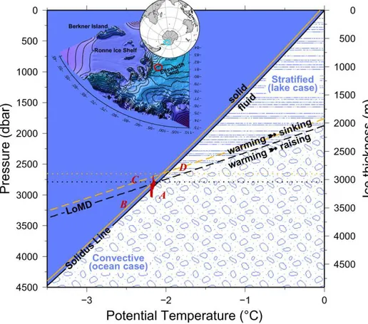
density maximum moves to lower temperatures if the pressure increases, as indicated by the dashed Line of Maximum Density (LoMD) in Fig. 1. Within subglacial lakes, water temperatures are close to the local pressure-dependent freezing point, indicated by the solidus line (solid line in Fig. 1). The ice thickness above a subglacial lake

15

determines the pressure at the ice-lake interface and hence where the lake is situated with respect to the LoMD. If the ice coverage is thinner than about 3050 m (pressure of about 2790 dbar), the bottom waters (heated by geothermal heat flux) are denser than the overlying colder waters, resulting in a stratified lake where warm water accumulates at the bottom (referred to aslake case). If the ice thickness exceeds this limit, warmer

20

bottom water becomes buoyant and rises to the surface, leading to the convective ocean case (W ¨uest and Carmack, 2000; Thoma et al., 2010b). In this context, it is important to note that even with the so-called stable temperature stratification (lake case) an inclined ice-lake interface slope induces water circulation within the lake due to buoyancy forces resulting from latent heat release in freezing zones and initiates

25

(7)

TCD

5, 1003–1020, 2011

SLE

M. Thoma et al.

Title Page

Tables Figures

◭ ◮

Back Close

Full Screen / Esc

Discussion

P

a

per

|

Dis

cussion

P

a

per

|

Discussion

P

a

per

|

Discussio

n

P

a

per

|

3.4 Temperature regimes in general and in Subglacial Lake Ellsworth

Many large subglacial lakes in Antarctica are buried by at least 3500 m of ice (Siegert et al., 2005; Smith et al., 2009). In these lakes, only two temperature regimes can be observed. Where the ice sheet is thickest, cold meltwater is released and amplifies the vertical mixing triggered by warmer rising bottom waters (indicated as regime A in

5

Fig. 1). In contrast, where the ice sheet is thinner, latent heat is released by freezing. This warmer water accumulates in a thin surface layer and stratifies the water column (regime B). These two regimes are the only ones present in the previously studied Subglacial Lakes Vostok and Concordia (Thoma et al., 2008b, 2009, 2010b). SLE is di_fferent and exceptional as it is covered by 2930 to 3280 m of ice and hence situated

10

exactly at the intersection between the solidus line and the LoMD (red-indicated area in Fig. 1). As a result, the LoMD crosses the water column in the lake. This generates the additional temperature regime C which is unique amongst currently surveyed sub-glacial lakes. Here the release of latent heat by freezing of supercooled waters leads to warming which increases the density and hence initiates sinking and mixing of the

15

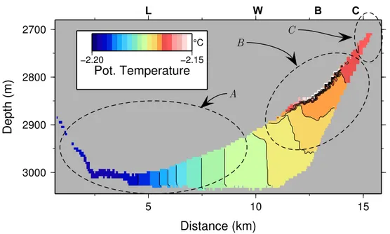
water masses. The location of all three temperature regimes within SLE is indicated in Fig. 3. Thetipping depth, where the LoMD intersects the surface, is indicated by the blue line in Fig. 2c. South of this tipping depth, the convective regime A and the strat-ified regime B are present as in other subglacial lakes, covered by much thicker ice. North of the tipping depth, within temperature regime C, downward mixing of warmer

20

water masses, generated by latent heat released at the ice-lake interface, results again in a vertically well-mixed water column (Fig. 3).

4 Discussion

4.1 Sensitivity to subglacial water flow

It is very likely that subglacial lakes are connected to each other. Several studies

in-25

(8)

TCD

5, 1003–1020, 2011

SLE

M. Thoma et al.

Title Page

Tables Figures

◭ ◮

Back Close

Full Screen / Esc

Discussion

P

a

per

|

Dis

cussion

P

a

per

|

Discussion

P

a

per

|

Discussio

n

P

a

per

|

to 20 m3s−1 _{(Gray et al., 2005; Fricker and Scambos, 2009). In some cases up to}

40 m3s−1 _{were estimated (Wingham et al., 2006; Fricker et al., 2007). Typical}

mod-elled volume transport within subglacial lakes ranges from 102 to 104m3s−1 _(Thoma

et al., 2010b). The specific strength is mainly determined by the lake’s volume and the surface slope. We estimate a volume mass transport of about 500 m3s−1_{for SLE (see}

5

the Supplement). Assuming subglacially flowing water is at its freezing point tempera-ture when entering a lake, no buoyancy forces are generated as no significant density (temperature) contrast appears. Hence, potential inflow generates mainly horizontal momentum. For SLE subglacial inflow may contribute to the internal circulation at a range of 0.2% to 8%. However, the energy balance between geothermal heat and

10

heat loss through the ice sheet as well as the slope of the ice-lake interface are the governing factors for the temperature regimes and the basal mass balance. Hence we suggest that subglacial water inflow has only a minor impact on the results presented here.

4.2 Sensitivity to water salinity

15

Salinity in subglacial lakes might enrich over time by refreezing of pure water or might intrude at the edges of the Antarctic Ice Sheet from the Southern Ocean. However, according to previous studies (Siegert, 2000; Souchez et al., 2000, 2003) the salinity in Subglacial Lake Vostok is very low (.1.2) or even zero (Gorman and Siegert, 1999; Priscu et al., 1999; Siegert et al., 2001). Assuming that a hydrological network

con-20

nects subglacial lakes and that the typical lake-water residence times (in the order of 104to 105yr) is comparable, there is no evidence that salinity in any other subglacial lake is significantly different. Even for subglacial lakes near the edge of the Antarc-tic Ice Sheet, the hydrological potential inhibits salt water intrusion from the Southern Ocean. To assess the sensitivity of the LoMD with respect to salinity, we assume a

25

salinity of 1‰. This moves the freezing point as well as the LoMD to lower ice thick-nesses (Fig. 1), and results in a criticaltipping depth of about 2900 m (≈2655 dbar).

(9)

TCD

5, 1003–1020, 2011

SLE

M. Thoma et al.

Title Page

Tables Figures

◭ ◮

Back Close

Full Screen / Esc

Discussion

P

a

per

|

Dis

cussion

P

a

per

|

Discussion

P

a

per

|

Discussio

n

P

a

per

|

4.3 Sensitivity to density variations and ice thickness

Assuming a solid ice column (with a constant density of 917 kg m−3_{) instead of an ice}

sheet with an overlying firn layer introduces an error with respect to the tipping depth. According to seismic measurements performed during the field campaign, the firn layer reaches to about 120 m depth in the SLE region (see the Supplement). Considering

5

this, the tipping depth increases by about 0.67% (or 20 m of ice). With respect to the findings in this manuscript, this deviation can be ignored.

Interpretations of trim lines in the Ellsworth Mountains suggest that the ice sheet was several hundred metres thicker during the Last Glacial Maximum (Bentley et al., 2010). This implies that SLE, assuming it existed at that time, had only two temperature

10

regimes (A and B) and has since experienced a regime shift. The unique regime C will have been established some time during the Holocene transition over the last 15 000 yr when the ice sheet became thinner. If the ice thickness should decrease further by about 150 m, the tipping depth, representing the critical pressure boundary, will move further out of the freezing zone and into the melting area. In this case, a

15

fourth temperature regime D will replace regime B (Fig. 1). A further ice-thickness reduction (of about 300 m to 450 m in total) would finally remove regime A completely from SLE. The difference between such a subglacial lake, covered by less than about 2700 m of ice, and a cold frozen surface lake is the inclined ice-lake surface, which still maintains a water circulation and hence the production of supercooled water with

20

freezing capabilities. Sensitivity studies of the impact of a decreasing ice-thickness on the basal mass balance, the lake’s surface temperature as well as the surface and basal flow of SLE are discussed and provided in the Supplement.

5 Conclusion with respect to SLE access locations

25

(10)

TCD

5, 1003–1020, 2011

SLE

M. Thoma et al.

Title Page

Tables Figures

◭ ◮

Back Close

Full Screen / Esc

Discussion

P

a

per

|

Dis

cussion

P

a

per

|

Discussion

P

a

per

|

Discussio

n

P

a

per

|

Our modelling results have immediate implications for proposed drill access into SLE and relevance for access into other lakes. For SLE, implications relate to the lake water, sediment retrieval and operational risk. Woodward et al. (2010) proposed one location for initial access; the new results in this paper suggest a number of alternative locations should also be considered, depending on scientific as well as operational priorities.

5

1. The presence of the tipping depth within SLE provides two unique opportunities: First, to improve our understanding of subglacial lake water dynamics, and sec-ond, to ratify, or further refine the EoS for water under otherwise inaccessible conditions of low salinity and high pressure. For these priorities, profiling the strongly stratified water column in regime B and the unique mixed column, driven

10

by freezing at the interface, in regime C, would be required. (These proposed access points are indicated by B and C in Figs. 2 and 3, respectively.) These would allow us to test and assess the accuracy of our model parameters and as-sumptions. In particular, the presence in SLE of regime C, as a consequence of the intersection of the tipping depth with the ice-water interface, would confirm its

15

theoretical prediction. From the perspective of the work in this paper, the top pri-ority measurements in SLE would therefore be temperature and salinity profiles of the water column at two locations in the basal freezing area (Fig. 2a), one in regime B at≈13 km and one in regime C at≈14.5 km along the profile in Fig. 3,

combined with borehole logging to confirm accreted ice thicknesses.

20

2. Detection of life in subglacial lakes is a prime motivation for direct access. Micro-bial concentrations within the water column itself may be low, but the sediments at the lake floor will contain a concentration of deceased organisms deposited over time. The optimum location to retrieve these samples will be where low wa-ter speeds have allowed maximum sedimentation rates at the lake floor. This

25

suggests a location ≈5 km from the southern end of the lake, where the model

(11)

TCD

5, 1003–1020, 2011

SLE

M. Thoma et al.

Title Page

Tables Figures

◭ ◮

Back Close

Full Screen / Esc

Discussion

P

a

per

|

Dis

cussion

P

a

per

|

Discussion

P

a

per

|

Discussio

n

P

a

per

|

history record, contained in a sediment core. To optimize that priority, Woodward et al. (2010) proposed a location at the downstream end of the area of basal melting (≈10 km in Fig. 3), where sedimentation rates were expected to be low.

3. We agree with an earlier conclusion Woodward et al. (2010) based on a simplified bathymetry, that access in the southern part of the lake poses the least operational

5

risk. The basal melting indicated there shows that access complications caused by basal freezing mechanisms will be avoided. (The access point proposed by Woodward et al. (2010) is indicated byW in Figs. 2 and 3.)

In summary, future efforts in accessing Antarctic subglacial lakes will definitely improve our understanding of subglacial lake dynamics and will most probably contribute to the

10

disclosing the secret of Antarctic history.

Supplementary material related to this article is available online at:

http://www.the-cryosphere-discuss.net/5/1003/2011/tcd-5-1003-2011-supplement. pdf.

Acknowledgements. This work was funded by the DFG through grant MA3347/2-1. The data

15

acquisition was funded by NERC-AFI NE/D008751/1, NE/D009200/1, NE/D008638/1. The authors wish to thank Martin Siegert for initiating the Lake Ellsworth proposal, David Vaughan, Martin Siegert, and two anonymous reviewers for helpful comments and discussions, as well as Andrea Bleyer and Marc Taylor for proof reading.

References

20

Bentley, M. J., Fogwill, C. J., Le Brocq, A. M., Hubbard, A. L., Sugden, D. E., Dunai, T. J., and Freeman, S. P. H. T.: Deglacial history of the West Antarctic Ice Sheet in the Weddell Sea embayment: constrains on past ice volume change, 38, 411–414, 2010. 1011

Dowdeswell, J. A. and Siegert, M. J.: The physiography of modern Antarctic subglacial lakes, Global Planet. Change, 35, 221–236, 2002. 1004

(12)

TCD

5, 1003–1020, 2011

SLE

M. Thoma et al.

Title Page

Tables Figures

◭ ◮

Back Close

Full Screen / Esc

Discussion

P

a

per

|

Dis

cussion

P

a

per

|

Discussion

P

a

per

|

Discussio

n

P

a

per

|

Filina, I. Y., Blankenship, D. D., Thoma, M., Lukin, V. V., Masolov, V. N., and Sen, M. K.: New 3D bathymetry and sediment distribution in Lake Vostok: Implication for pre-glacial origin and numerical modeling of the internal processes within the lake, Earth Planet. Sc. Lett., 276, 106–114, doi:10.1016/j.epsl.2008.09.012, 2008. 1004, 1005

Fricker, H. A. and Scambos, T.: Connected subglacial lake activity on lower Mercer

5

and Whillans Ice Streams, West Antarctica, 2003–2008, J. Glaciol., 55, 303–315, doi:10.3189/002214309788608813, 2009. 1004, 1010

Fricker, H. A., Scambos, T., Bindschadler, R., and Padman, L.: An active subglacial water system in West Antarctica mapped from space, Science, 315, 1544–1548, doi:10.1126/science.1136897, 2007. 1010

10

Gorman, M. R. and Siegert, M. J.: Penetration of Antarctic subglacial lakes by VHF electro-magnetic pulses: Information on the depth and electrical conductivity of basal water bodies, J. Geophys. Res., 104, 29311–29320, 1999. 1010

Gray, L., Joughin, I., Tulaczyk, S., Spikes, V. B., Bindschadler, R., and Jezek, K.: Evidence for subglacial water transport in the West Antarctic Ice Sheet through three-dimensional satellite

15

radar interferometry, Geophys. Res. Lett., 32, L03501, doi:10.1029/2004GL021387, 2005. 1010

Holland, D. M. and Jenkins, A.: Modeling Thermodynamic Ice-Ocean Interaction at the Base of an Ice Shelf, J. Phys. Oceanogr., 29, 1787–1800, 1999. 1006

Jackett, D. R., McDougall, T. J., Feistel, R., Wright, D. G., and Griffies, S. M.: Algorithms for

20

density, potential temperature, conservative temperature, and the freezing temperature of seawater, J. Atmos. Ocean. Tech., 23, 1709–1728, doi: 10.1175%2FJTECH1946.1, 2006. 1006, 1007, 1008, 1017

Maule, C. F., Purucker, M. E., Olsen, N., and Mosegaard, K.: Heat flux anomalies in Antarctica revealed by satellite magnetic data, Science, 309, 464–467, doi:10.1126/science.1106888,

25

2005. 1007

Pattyn, F.: A new three-dimensional higher-order thermomechanical ice sheet model: Basic sensitivity, ice stream development, and ice flow across subglacial lakes, J. Geophys. Res., 108, 1–15, doi:10.1029/2002JB002329, 2003. 1005

Pattyn, F.: Investigating the stability of subglacial lakes with a full Stokes ice-sheet model, J.

30

Glaciol., 54, 353–361, doi:10.3189/002214308784886171, 2008. 1005

(13)

TCD

5, 1003–1020, 2011

SLE

M. Thoma et al.

Title Page

Tables Figures

◭ ◮

Back Close

Full Screen / Esc

Discussion

P

a

per

|

Dis

cussion

P

a

per

|

Discussion

P

a

per

|

Discussio

n

P

a

per

|

Geomicrobiology of Subglacial Ice Above Lake Vostok, Antarctica, Science, 286, 2141–2144, doi:10.1126/science.286.5447.2141, 1999. 1010

Shapiro, N. M. S. and Ritzwoller, M. H.: Inferring surface heat flux distributions guided by a global seismic model: particular application to Antarctica, Earth Planet. Sc. Lett., 223, 213– 224, doi:10.1016/j.epsl.2004.04.011, 2004. 1007

5

Siegert, M. J.: Antarctic subglacial lakes, Earth Sci. Rev., 50, 29–50, 2000. 1008, 1010 Siegert, M. J., Ellis-Evans, J. C., Tranter, M., Mayer, C., Petit, J.-R., Salamatin, A., and Priscu,

J. C.: Physical, chemical and biological processes in Lake Vostok and other Antarctic sub-glacial lakes, Nature, 414, 603–609, 2001. 1010

Siegert, M. J., Tranter, M., Ellis-Evans, J. C., Priscu, J. C., and Lyons, W. B.: The

hydrochem-10

istry of Lake Vostok and the potential for life in Antarctic subglacial lakes, Hydrol. Process., 17, 795–814, 2003. 1004

Siegert, M. J., Carter, S., Tabacco, I. E., Popov, S., and Blankenship, D. D.: A revised inventory of Antarctic subglacial lakes, Antarct. Sci., 17, 453–460, doi:10.1017/S0954102005002889, 2005. 1009

15

Smith, B. E., Fricker, H. A., Joughin, I. R., and Tulaczyk, S.: An inventory of active subglacial lakes in Antarctica detected by ICESat (2003–2008), J. Glaciol., 55, 573–595, 2009. 1009 Souchez, R., Petit, J. R., Tison, J. L., Jouzel, J., and Verbeke, V.: Ice formation in subglacial

Lake Vostok, Central Antarctica, Earth Planet. Sc. Lett., 181, 529–538, 2000. 1005, 1010 Souchez, R., Petit, J. R., Jouzel, J., DeAngelis, M., and Tison, J.: Re-assessing lake Vostok’s

20

behavior from existing and new ice core data, Earth Planet. Sc. Lett., 217, 163–170, 2003. 1008, 1010

Thoma, M., Grosfeld, K., and Mayer, C.: Modelling accreted ice in subglacial Lake Vostok, Antarctica, Geophys. Res. Lett., 35, 1–6, doi:10.1029/2008GL033607, 2008a. 1006

Thoma, M., Mayer, C., and Grosfeld, K.: Sensitivity of Lake Vostok’s flow regime on

environ-25

mental parameters, Earth Planet. Sc. Lett., 269, 242–247, doi:10.1016/j.epsl.2008.02.023, 2008b. 1006, 1008, 1009

Thoma, M., Filina, I., Grosfeld, K., and Mayer, C.: Modelling flow and accreted ice in subglacial Lake Concordia, Antarctica, Earth Planet. Sc. Lett., 286, 278–284, doi:10.1016/j.epsl.2009.06.037, 2009. 1005, 1009

30

(14)

TCD

5, 1003–1020, 2011

SLE

M. Thoma et al.

Title Page

Tables Figures

◭ ◮

Back Close

Full Screen / Esc

Discussion

P

a

per

|

Dis

cussion

P

a

per

|

Discussion

P

a

per

|

Discussio

n

P

a

per

|

Thoma, M., Grosfeld, K., Smith, A. M., and Mayer, C.: A comment on the equation of state and the freezing point equation with respect to subglacial lake modelling, Earth Planet. Sc. Lett., 294, 80–84, doi:10.1016/j.epsl.2010.03.005, 2010b. 1008, 1009, 1010

Tikku, A. A., Bell, R. E., Studinger, M., Clarke, G. K. C., Tabacco, I., and Ferraccioli, F.: Influx of meltwater to subglacial Lake Concordia, east Antarctica, J. Glaciol., 51, 96–104, 2005. 1004

5

Vaughan, D. G., Rivera, A., Woodward, J., Corr, H. F. J., Wendt, J., and Zamora, R.: Topo-graphic and hydrological controls on Subglacial Lake Ellsworth, West Antarctica, Geophys. Res. Lett., 34, 1–5, doi:10.1029/2007GL030769, 2007. 1008

Wingham, D. J., Siegert, M. J., Shepherd, A., and Muir, A. S.: Rapid discharge connects Antarctic subglacial lakes, Nature, 440, 1033–1036, doi:10.1038nature04660, 2006. 1010

10

Woodward, J., Smith, A. M., Ross, N., Thoma, M., Corr, H. F. J., King, E. C., King, M. A., Grosfeld, K., Tranter, M., and Siegert, M. J.: Location for direct access to subglacial Lake Ellsworth: An assessment of geophysical data and modeling, Geophys. Res. Lett., 37, L11501, doi:10.1029/2010GL042884, 2010. 1005, 1006, 1012, 1013, 1019

Wright, A. and Siegert, M. J.: The identification and physiographical setting of Antarctic

sub-15

glacial lakes: an update based on recent geophysical data, in: Subglacial Antarctic Aquatic Environments, edited by: Siegert, M. J., Kennicutt, C., and Bindschadler, B., AGU Mono-graph, 28 pp., 2010. 1005

Wright, D. G., Feistel, R., Reissmann, J. H., Miyagawa, K., Jackett, D. R., Wagner, W., Overhoff, U., Guder, C., Feistel, A., and Marion, G. M.: Numerical implementation and oceanographic

20

application of the thermodynamic potentials of liquid water, water vapour, ice, seawater and humid air - Part 2: The library routines, Ocean Sci., 6, 695–718, doi:10.5194/os-6-695-2010, 2010. 1006, 1007

W ¨uest, A. and Carmack, E.: A priori estimates of mixing and circulation in the hard-to-reach water body of Lake Vostok, Ocean Model., 2, 29–43, 2000. 1005, 1008

(15)

TCD

5, 1003–1020, 2011

SLE

M. Thoma et al.

Title Page

Tables Figures

◭ ◮

Back Close

Full Screen / Esc

Discussion

P

a

per

|

Dis

cussion

P

a

per

|

Discussion

P

a

per

|

Discussio

n

P

a

per

|

Fig. 1. Inlay: surface topography in the area of SLE, indicated with the red circle. Contours are 200 m apart. Main

figure: solidus line (solid) and line of maximum density (LoMD, dashed) (Jackett et al., 2006) as well as the parameter space where SLE is located (red). The ice thickness refers to a density of 917 kg m−3_{. The four possible temperature}

(16)

TCD

5, 1003–1020, 2011

SLE

M. Thoma et al.

Title Page Abstract Introduction Conclusions References Tables Figures ◭ ◮ ◭ ◮ Back Close

Full Screen / Esc

Printer-friendly Version Interactive Discussion Discussion P a per | Dis cussion P a per | Discussion P a per | Discussio n P a per | 2950 m 3

000_m

30₅₀ m 3₁ 0₀ m 3 1 0 0 m 315 0 m

31 50

m

32₀

0 m

3₂

5 0 m

5 mm/s

2 km

0 100 200

Water Column m N C B W L a) −20 −10 −10 0 0 10 10 2030 30 5 mm/s 2 km

−30 0 30

Basal Mass Balance

cm/a N C B W L b) −2.19 −2.18 −2.17 −2.16 −2.16 −2.16 −2.16 −2.15 −2.15 −2.14 5 mm/s 2 km −2.20 −2.15 Pot. Temperature °C N C B W L

c) 295₀

m

3

000_m

30 50_m

3₁ 0 0 m 3 1 0 0 m 315 0 m

31 50

m

32 0₀m 3

2_{5 0}m

2 km

10−1 ₁₀0 ₁₀1 ₁₀2 Accreted Ice m N C B W L d)

(17)

TCD

5, 1003–1020, 2011

SLE

M. Thoma et al.

Title Page

Tables Figures

◭ ◮

Back Close

Full Screen / Esc

Discussion

P

a

per

|

Dis

cussion

P

a

per

|

Discussion

P

a

per

|

Discussio

n

P

a

per

|

Fig. 2. (a)Water column thickness (colour coded) and ice thickness (red contours) of SLE

according to Woodward et al. (2010). The yellow line indicates the cross section path shown in Fig. 3. Arrows indicate flow in the bottom layer.(b)Modelled basal mass balance at the ice-lake interface. Negative values indicate melting, positive values freezing. Arrows indicate the flow in the middle of the water column.(c)Modelled lake temperature at the ice-lake interface. The bluetipping depthline indicates the area where the line of maximum density (LoMD) intersects the ice-lake interface. Arrows indicate water flow at the ice-lake interface.(d)Modelled accreted ice thickness, assuming an ice flow of 5.5 m a−1_{. Arrows indicate ice flow direction. The green}

(18)

TCD

5, 1003–1020, 2011

SLE

M. Thoma et al.

Title Page

Tables Figures

◭ ◮

Back Close

Full Screen / Esc

Discussion

P

a

per

|

Dis

cussion

P

a

per

|

Discussion

P

a

per

|

Discussio

n

P

a

per

|

2700

2800

2900

3000

Depth (m)

5 10 15

Distance (km)

L W B C

−2.20 −2.15

Pot. Temperature °C

A B

C

Fig. 3.Temperature cross section along the path shown in Fig. 2. Different temperature regimes