Is Africa’s current growth reducing inequality? Evidence from some selected african countries

(1)

Is Africa’s

current growth reducing inequality? Evidence from

some selected african countries

Alege P.O. George E.O. Ojeaga P.I. Oluwatimiro Q.

Covenant University Nigeria P.M.B 1023 Ota Department of Economics and Development Studies

Abstract

Is Africa’s current growth reducing inequality? What are the implications of growth on output performances in Africa? Does the effect of Africa’s growth on sectorial output have any implication for inequality in Africa? The study investigates the effect of shocks on a set of macroeconomic variables on inequality (measured by life expectancy) and the implication of this on sectors that are perceived to provide economic empowerment in form of employment for people living in the African countries in our sample. Studies already find that growth in many African countries has not been accompanied with significant improvement in employment. Therefore inequality is subject to a counter cyclical trend in production levels when export destination countries experience a recession. The study also provides insight on the effect of growth on sectorial output for three major sectors in the African economy with the intent of analyzing the impact of growth on sectorial development. The method used in this study is Panel Vector Autoregressive (PVAR) estimation and the obvious advantage of this method lies in the fact that it allows us to capture both static and dynamic interdependencies and to treat the links across units in an unrestricted fashion. Data is obtained from World Bank (WDI) Statistics for the period 1985 to 2012 (28 years) for 10 African Countries. Our main findings confirm strong negative relationship between GDP growth and life expectancy and also for GDP and the services and manufacturing sector considering the full sample.

Keywords:Growth, Sectorial Performances, Inequality, Panel VAR and Africa

JEL Classification: C33, E30, F62

1. Introduction

In this section a brief introduction into growth and inequality is presented. According to the World BankăpressăreleaseăOctoberă2013,ăAfrica’săeconomicăgrowthăoutlookăcontinuesătoăremainăstrongăwithăană estimated forecast of 4.9% growth rate for 2013, it is expected that the African economy will grow by 6% in 2014, depicting that Africa will continue to experience strong economic growth in the years to come. The African region is also expected to remain a strong magnet for tourism and investment due to the attractiveness of the African business environment despite problems of high political instabilit y, business environment risks and poor economic policies. Strong government investments, higher production in the mineral, agricultural and services sectors are also boosting growth in many African countries. Private investment and regional remittances are also on the increase, with remittances alone now worth over 33 billion dollars supporting household income. It is clear that almost a third of the countries in the region are now experiencing growth rates of over 6% making African countries to be among th e fastest growing economies in the world. This increasing growth trends however, have also been found not to translate to poverty reduction in many African countries. Inequality and poverty has remained quite high despite strong growth and the rate of poverty reduction has remained quite sluggish, with Africa still accounting for the highest proportion of un-enrolledă schoolă childrenă ină theă World.ă Africa’să Pulseă (2014)ă aă Worldă Bank yearly Journal, also states that despite the global economic improvement in A frica, poverty will continue to remain a strong concern on the continent. Forecasting that between 16 to 33% of the entire World’săpoor,ăwillăresideăinăAfricaăbyă2030ăpresentingăonceăagainăaăfutureădemographicăchallengeăthată can be an impediment to future development of the continent. The vulnerability of economic growth in Africa to capital flow and commodity price reduction also makes it imperative for many African countries



(2)

to invest in times of growth in other non-performing sectors with prospects for cushioning their economies from global shocks (i.e. shocks associated with a sudden reduction in commodity prices and capital flows to the continent).

This paper investigates the effects of growth on inequality in Africa by studying the implication of growth for sectors in the African economy that are labor intensive particularly the agricultural and services sector with meaningful use for economic empowerment and inequality reduction. It also investigates the effect of growth on the manufacturing sector that is less labor intensive with the intent understanding the impact of growth on the manufacturing sector. Incite is gained on the implication of growth on inequality reduction in general using panel vector auto regression (PVAR) which allows us to study dynamic interdependencies between growth and inequality reduction with the intent of establishing a link between growth and inequality the impact of growth on sectorial output particularly for sectors with capability for employment are also considered. Data for some ten selected African countries (they include Algeria, Egypt, Ghana, Nigeria, Kenya, Uganda, Cameroon and Congo) two from each major economic regions (i.e. North, West, East, Central, and Southern Africa) in Africa is utilized in the study for th e period of 1985 to 2012 a period of 28 years. The rest of the paper is divided into the scope and objective, review of literature, empirical analysis and results and the concluding sections.

2. Scope and Objectives of the Study

In this section the scope and objectives of the study are presented. The study investigates the implications of the current growth trend in Africa on inequality reduction, by studying the implications of growth on life expectancy (as the measure for inequality) and output productio n in three sectors namely agricultural, services and the manufacturing sectors, the first two being labour intensive and the last a technological driven sector termed high-tech under the assumption increased productivity in sectors will mean higher levels of economic empowerment through employment. The objectives of the study are:

a. ToădetermineătheăeffectăofăAfrica’săcurrentăgrowthăonăinequalityăreduction

b. ToăevaluateătheăeffectăofăAfrica’săgrowthăonăsectorialăperformancesăinăthreeămajorăsectorsăină the African economy i.e. agricultural, services and manufacturing sectors.

c. Andă toă investigateă ifă theă impactă ofă Africa’să currentă growthă hasă ană effectă onă laboră intensiveă sectors with the capability to reduce inequality.

3. Stylized Facts on Growth and Inequality

(3)

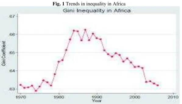
Fig. 1 Trends in inequality in Africa

Note: The graph above depicts that inequality is on the decrease this is particularly noticeable from the early 1990s. However Africa still has the World’s highest percentage of people living below the

poverty line.

Source: World Bank Gini-coefficient on inequality in Africa

Trends already show that there is still a wide gap between the rich and the poor in Africa; although inequality is reducing (See Trends in inequality in Fig. 1), Africa still has the highest per cent of the world’săpeopleălivingă below the poverty line. This depicts the sluggishness of government policies in yielding results that can have meaningful effect for job creation and skill improvement. The paper by Art Kraay (2004) after studying the implication of growth for household income in some selected developing countries also state that at best, there is a negative relationship between annual average growth and annual growth in household in many developing countries depicting that national growth does not often translate to household growth in developing countries thereby suggesting a counter-cyclical relationship between growth and annual household growth. This shows that growth in many developing countries are often not inclusive, and are associated with joblessness therefore such economic expansions are not characterized

Fig.2 Relationship between growth rate and poverty reduction

Note: The fig above depicts that national growth does not often translate to household growth in many African countries suggesting a counter-cyclical relationship between growth and annual household growth.

(4)

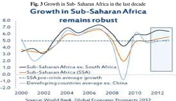
with improved skill development and training of indigenous manpower in many developing countries. Trends also show that growth rate in sub Saharan Africa remains modestly high particularly in the last decade according toătheăWorldăBankăstatisticsă2013ă(seeăfig.ă3),ăAfrica’săgrowthărateăhasăbeenăonătheăaverageăatăapproximatelyă6%ă annually. Pundits also state that though the growth trend has lasted for close to a decade many African countries have failed to take advantage of the current trend to diversify their economics from simple raw material exporting economies to middle level manufacturing economies.Despite the less developed nature of the African banking system compared to those of the developed North, the 2008 financial meltdown had strong effects on the economies of many African countries. Depicting an interdependent relationship, between Africa and the rest of the World.

Fig. 3 Growth in Sub- Saharan Africa in the last decade

Note:ăTheăfigureăaboveăshowsărecentătrendsăinăgrowthăforătheălastădecadeăinăAfrica.ăAfrica’săgrowthărateăhasăbeenăonătheăaverage at approximately 6% annually. This growth is often associated with sustained commodity price boom. It also shows the interdependency between the

developed North and developing South particularly the effect of the sub-prime mortgage crisis of 2008 on growth in Africa.

Growth in the last decade has also managed to surpass that of the 1980s (see Fig. 4), this increasing trend in growth has not translated to improved earnings for the mass of the population in many African countries. The long run implication of such growth for Africa is that productive capabilities are going to be limited in the future as natural resources dwindle. It also means that in the short run many African countries are going to continue to trade in primary goods (raw material exports), obviously missing out from gains often associated with product differentiation that skill and development of a robust domestic industrial base can provide.

(5)

Fig. 4. Graph of poverty rate and GDP in Sub-Saharan Africa

Note: The above graph depicts the counter-cyclical nature of Poverty on GDP in Africa. This depicts that improved growth showing in the last decade i.e. year 2000 onwards has not translated to strong reduction in the income gap between the rich and poor in many African countries.

Source: World Bank data

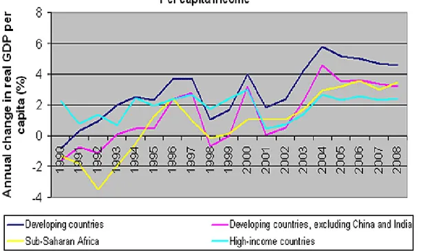
Trends also suggest that there is a relationship in movements in GDP across the different regions of the world see Fig. 5. Financial shocks are also seen to be transmitted from high income countries to other regions in subsequent periods. This once again depicts the interdependent nature of the global economy. Capital flows in times of economic shock can have strong effects for many developing countries receiving foreign aid, so also can it affect foreign direct investment to the private sector of the economies of many developing countries since investors are often known to repatriate funds back to their domestic economies in times of crisis. The implication of such negative capital flows is that a reduction will in turn affect the volume of their expenditure spending. This reduces their capability of providing social infrastructure and other social amenities which have the tendency to reduce the gap between the rich and poor.

Fig. 5 GDP per capita in Developed, Developing and African Countries

Note: The figure above compares GDP in high income countries to those of other developing countries and Africa. Financial shocks are seen to be transmitted from high income countries to other regions in subsequent periods. This once again depicts the interdependent nature of the global

economy.

(6)

4. Review of Literature

In this section we review some past literature on the subject under study. Past studies have utilized panel regressions in studying, the effect of capital flows particularly in times of banking crisis on aid supply and find that aid supply decreases after the first two periods in times of crisis Laeven and Valencia (2010). Historical evidences of the effect of capital flows have found that recessions are likely to have deep and prolonged effects on growth and fiscal balance and cause significant disturbances to government revenue and expenditure Reinhart and Roghoff (2008).

The variables used in the study are based on instrumental variables for poverty (life expectancy, Misery index etc) and aid Hansen and Tarp (2001), Rajan Subramanian (2008) and Ojeaga (2012). VAR models are also employed, the models employed in the paper by Frot (2009) is extended for the purpose of the study. The variables employed in the analysis in the study have been found to have significant relevance for life expectancy in one or more past literature. They include GDP per capita, fiscal variables such as government expenditure spending and sectorial output from manufacturing, services and agriculture see Chong and Granstein (2008), Faini (2006), Boschini and Olofsgard (2007) Dang et al (2009) and Frot (2009).

The aim of the study is to investigate the extent to which capital flows affect inequality in Africa using data from some selected countries and compare the response of life expectancy and output productivity particularly in three sectors that can influence economic empowerment which include the agricultural, manufacturing and services sectors to unexpected shocks. It is worthy of note to state also that other studies have presented counter argument rejecting the possible relationship between decreases in capital flows and economic recessions stating that capital flows does not depend solely on economic factors, arguing that political factors and strategic decisions about where to invest were more relevant see

Paxton and Knack (2008) for such a critical position

. However, in this study, it was found that economic factors influence capital flows and significantly affects fiscal spending which in turn have grave consequences for inequality.

5. Empirical Analysis and Results

5.1. Theoretical Framework

In this subsection the theoretical frameworkă ofă theă studyă isă presented.ă Weă assumeă thatăthereăareă i=1,…..tă sectors in the economy of countries, contributing to their aggregate output production of which export is a useful fraction and that exports from countries will flow to different export destinationăcountriesăj=ă1,……j.ăPrivateă sector production is also not purely to promote welfare and production of satisfactory public goods in countries but mainly for the private interest (profits for the private entrepreneur) which is the returns on invested revenue i.e. firms profit maximization ends. Therefore firms in countries are indirect consumers of production. The framework portrays aggregate production therefore as a private rather than a public good. Large firms will therefore produce fewer goods per total revenue than small firms, since large numbers of shareholders will mean more profits shared, rather reinvested in the production process. The aim of this paper is to investigate, the effect of the choice of producers to consume indirect production or maximize welfare. Therefore we can let the producers in sectors have the utility function expressed in equation 1 as

(1) _, = f (� _, _, )

Where � _, is aggregate production in a country across sectors j in firm i at time t, and _, is the total consumption in firm i at time t. Individual preferences for firm goods can be written as expressed by Chong and Gradstein (2008) as

(2) U= _� (� _, ) + _, =

−� � , −� + −� , −� , >

The parameter is the preferences for goods produced and � is the elasticity of substitution between two goods. Income is also allocated between consumption, government expenditure and firms, therefore if price is numeraire, then firms budget constraint will be

(7)

Where represents preferences for internal expenditures and _, represents cost of transaction between firms and markets (external expenditure). Revenues _. come from sales _. and from bank credit _. that are used to finance production and other firm internal costs, expressed as

(4) _. = _. + _.

(5) _. = � _, + _, = _,

Therefore firm output will follow production targets across sectors representing aggregate output in countries which will be subject to external shocks and deviation, where the adjustment to such shocks will take longer than one period. The production of goods by firms i in countries will be subject to available resources for production and other internal cost incurred by firms in their day to day production. Such cost related to unstable economic conditions will affect production levels � _{, −} and could also be associated with other long run impacts expressed as the lagged variables of the internal cost of firms _{, −} . Allowing us to state production below as

(6) � _, = � _{, −} ∑,₌ _,

= ∑ , −

, =

= �, �,

With �_, representing, other country or time specific shocks, and s indicating the number of lagged periods. The impact of crisis shocks will be function firms internal needs, financial condition of consuming countries and exporting countries, social conditions in producing countries and other political preferences.

(7) _, = _, ; _, ; _,

Production will be an increasing function of good financial conditions, political concerns, social conditions and available resources and decreasing function of social needs since firms having their own profit maximizing interests expressed below as

(8) ��

� < , ��

� > , ��

� > , �� >

5.2. Empirical Analysis

In this subsection the intuition for the study is presented. The analysis is based on VAR, it adequately stems from the fact that it studies interdependencies among variables without worrying about the direction of causality. It is flexible and the method treats all variables in the system as endogenous and independent, each variable is explained by its own lagged values and those of the other variables.

It is also a system of equations and not a one equation model. Panel VAR also allows for the investigation of unobservable individual heterogeneity and improve asymptotic results. The results provide useful insights which go beyond coefficients to reveal the adjustment and resilience of unexpected production shocks as well as the importance of other different shocks. Canova and Ciccarelli (2004), give a brief description of the PVAR analysis expressing the general form as

(9)

_,

=

�

_,

+

_{, −}

+…….+ă

_{, −}

+

where _, isăaăkx1ăvectorăofăkăpanelădataăvariables,ăandăi=ă1,……,ăI,ă _, is a vector of deterministic terms such as the linear trend, dummy variables or a constant, � isătheăassociatedăparameterămatrixăandătheăăL’săareăkăxă k parameter matrices attached to the lagged variables _, . The lag order is represented by p, the error process is represented by three components, _, the country specific effect, the yearly effect and �_, the disturbance term. Two restrictions are imposed by the specification: a.) It assumes common slope coefficients, and it does not allow for interdependencies across units. Therefore the estimates L are interpreted as average dynamics in the response to shocks. All variables depend on the past of all variables in the system as with the basic VAR model with the individual country specific terms been the difference.

(8)

volumes. There are other studies that have studied the effect of aid in times of crisis e.g. Gravier-Rymaszewska (2012), Hansen and Heady (2010) also study the effect of aid on net imports and spending using PVAR.

The study uses PVAR approach to estimate the effect on inequality and sectorial production output of unexpected shocks to a set of variables that are responsive to economic upturns. The method is suitable since the VAR method does not require the imposition of strong structural relationship and another merit is that only a minimal set of assumptions are needed to interpret the impact of shocks on each variable. The reduced form equation allows for the implementation of dynamic simulations once the unknown parameters are estimated. However the method only allows for the analysis of short run adjustments effects and not the long run structural effects.

The results come in form of the impulse response functions (IRFs) and their coefficients analysis as well as their forecast error variance decompositions (FEVDs) which allows for the examination of technological innovations or shocks to any variable in question to other variables. Orthogonalizing the response allows us to identify the effect of one shock at a time while others are held constant. The Choleski decomposition method of variance covariance matrix of residuals is adopted, the identification is based on the premise that variables which appear earlier in the system are more exogenous than those which appear later and are assumed endogenous. Implying that the variables that follow are affected by the earlier variables contemporaneously with lags and the later variables affect previous variables only with lags.

The simple VAR model is presented below with three variables: GDP per capita, government spending (govspend) and sectorial output (Sec.Out/GDP) as a percentage of GDP interchangeably with inequality although we emphasize on sectorial output for brevity in explanations, in the above order required for the VAR system estimation. Therefore GDP per capita is the most exogenous variable and production output from sectors as a percentage of GDP and inequality as the case maybe are the most endogenous variables. Output from sectors is endogenously affected by GDP and government spending (particularly on infrastructural development which has the capability of attracting FDI through the provision of enabling environment); higher GDP will mean probably higher output from sectors ordinarily.

A sector is not likely to affect GDP adversely particularly in economies with multiple sectors however diminished social infrastructural provision due to diminished government spending on social infrastructure will mean poor FDI inflow is likely to affect GDP making capital inflow into the economy a buffer for effects of shocks from sectorial output to aggregate GDP. The model interpretation requires a delay in the direct observation of sectorial output and profits attributable to firms given the business environment, therefore GDP will only respond to sectorial performances with lag. The three variable model is a simple model that contains GDP per capita, government spending and sectorial outputs Sec. out/GDP expressed in this particular order for the identification of the VAR system.

GDP per capita , govspend, _�. , .

This allows us to state that a set of endogenous equations influence each other therefore sectorial output is contemporaneously affected by GDP and government Spending. Lower GDP will therefore result in lower output in firms and lower FDI inflows due to poor social infrastructural provision will affect firm capacity to produce also. Theoretically therefore GDP will respond only to sectorial outputs from past periods. The three variable PVAR model is presented below as

[ ]

[

∆ � ,

∆ . ,

∆SEC_�

, ]

= [ ] + [ ]

[

∆ � , −

∆ . , −

∆SEC_�

, − ] + [ ]

Where _, is a 3 variable vector including 3 endogenous variables: GDP per capita ∆ � , government

spending ∆ . and sectorial outputs ∆SEC

(9)

sectorial outputs to shocks in GDP and government spending are subjects of strong interests in the study see Gravier-Rymaszewska (2012) for further discussion.

5.3. Data Presentation

In this subsection the data for the study is presented. The VAR estimation technique requires that the data is transformed to remove the trend and only keep data with variations. Employing the use of panel data ensures that the underlying structure is the same for each cross sectional unit .i.e. the matrices L coefficients are the same for all the countries in the sample. Fixed effects ( ) are introduced to overcome the restriction of the above constraint and allow for country heterogeneity. The limitations that the fixed effects are correlated with the regressors due to the use of lags of the dependent variables (Arellano and Bond 1991; Blundell and Bond 1998), makes us adopt a procedure called the Helmert transformation, a forward mean-differencing to eliminate the fixed effects (Arellano and Bover 1995) to keep the orthogonality between variables and their lags so that lags can be employed as instruments.

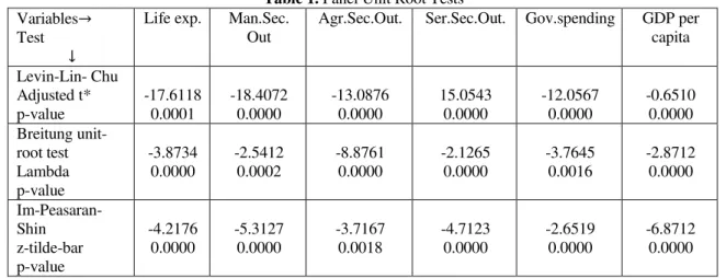
The issue of cross-sectional autocorrelation is dealt with by subtracting from each series at any time the average of the group see Levin and Lin (2002), for cross-sectional auto-correlation related to the common factors. The model is run in first difference to emphasize on the dynamics of sectorial output (and life expectancy as the case maybe) adjustments to and short run effects of shocks. The data is tested for stationarity in order to proceed with panel VAR. The data is in fact stationary as they are in first differences although the test is carried out for scrutiny. The main variables of interest GDP per cap, government spending, and sectoral output from sectors. Data for some ten selected African countries (they include Algeria, Egypt, Ghana, Nigeria, Kenya, Uganda, Cameroon and Congo) two from each major economic regions (i.e. North, West, East, Central, and Southern Africa) in Africa is utilized in the study for the period of 1985 to 2012 a period of 28 years all obtained from World Bank Data, are found to be stationary after conducting the Levin and Lin (2002), the Breitung (2001) and the Im, peaseran snd Shin (2003) unit root test . These are reported in the table below. It is therefore appropriate based on these test to proceed by estimating the model with panel VAR models.

Table 1. Panel Unit Root Tests Variables

Test

Life exp. Man.Sec. Out

Agr.Sec.Out. Ser.Sec.Out. Gov.spending GDP per capita

Levin-Lin- Chu Adjusted t* p-value

-17.6118 0.0001

-18.4072 0.0000

-13.0876 0.0000

15.0543 0.0000

-12.0567 0.0000

-0.6510 0.0000 Breitung

unit-root test Lambda p-value

-3.8734 0.0000

-2.5412 0.0002

-8.8761 0.0000

-2.1265 0.0000

-3.7645 0.0016

-2.8712 0.0000

Im-Peasaran-Shin z-tilde-bar p-value

-4.2176 0.0000

-5.3127 0.0000

-3.7167 0.0018

-4.7123 0.0000

-2.6519 0.0000

-6.8712 0.0000

Note: : Panels contain unit roots : Panels are stationary Common AR parameter

Number of panels = 10

Number of periods = GDP per capita (27) le (27) Gov. spending (25) Agr. Sec. out. (25) Man. sec. out.(24) Ser. Sec. out (24)

Source: Authors Compilations

5.4. Discussion of Results

(10)

economic empowerment. Our main findings confirm strong negative relationship between GDP growth and life expectancy considering the whole sample. The response of life expectancy to GDP shocks is stronger and significant in the second lag of GDP. This suggests that improvement in GDP growth does not cause any reasonable improvement in inequality reduction since government spending were not sufficiently reducing mortality rates in countries.

While GDP explains more of the government expenditure spending pattern in countries, negative GDP shocks are likely to account for up to 15% of government spending reduction in countries. The impulse response function gives us information on the short run dynamics of shocks impact. Most shocks start to have noticeable influences on the economy after the third lag and are likely to be absorbed probably 4 to 5 periods later. Our analysis of results suggests that shocks trigger structural changes, while government spending is negatively affected by GDP shocks, spending are likely to become more resilient after adjustments to shocks, therefore in times of growth expenditure spending are also likely to increase. The transmission of GDP shocks to inequality therefore is likely to be through expenditure spending on social welfare and infrastructural provision which despite increased growth in recent time has not sufficiently improved living conditions in many African countries

Finally, on extending the model to three sectors (the agricultural sector, services sector and manufacturing sectors) that have the capability to provide economic empowerment, we find that economic fluctuations decreases government spending and introduces a level of uncertainty to output production in sectors, government fiscal and monetary policies were found to have strong consequences on inequality and expenditure spending decisions, therefore these economic variables and government decisions were largely shaping inequality in countries.

System GMM Main Results for the Three Variable PVAR Model

Table 2. Full Sample Regression for Life Expectancy SHOCKS

Response of Response to

�−

Response to

. −

Response to

�−

Response to

. −

Life.exp. -.00002 (.00002) t=-.9023

-.0013 (.0008)* t=-1.7051

-.00010 (.00002)***

t=-3.8957

.0006 (.0009) t=.6934

Notes: ***indicates 1 percent significance level t-test> . : ** 5 percent significance level t-test > .9 , * 10 percent significance level t-test > . respectively. All standard errors are in parenthesis. The model is estimated by system GMM, while the country fixed effects and common factors are

remover before estimation.

Table 3. Full Sample Regressions for Manufacturing Sector Output SHOCKS

�−

Response to

. −

Response to

�−

Response to

. −

Manufacturing Output

.0001 (.0100)

t=.01

-.0065 (.5030) t=.0130

-.0010 (.0010) t=.01

-.0267 (.0854) t=.313

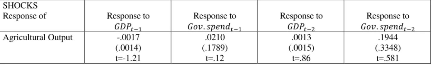
Table 4 Full Sample Regression for Agricultural Sector Output SHOCKS

�−

Response to

. −

Response to

�−

Response to

. −

Agricultural Output -.0017 (.0014) t=-1.21

.0210 (.1789)

t=.12

.0013 (.0015)

t=.86

.1944 (.3348)

t=.581

(11)

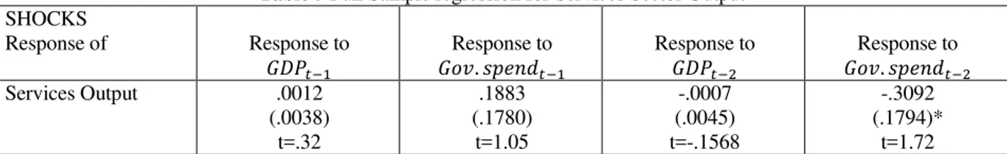
Table 5 Full Sample regression for Services Sector Output SHOCKS

�−

Response to

. −

Response to

�−

Response to

. −

Services Output .0012 (.0038)

t=.32

.1883 (.1780)

t=1.05

-.0007 (.0045) t=-.1568

-.3092 (.1794)*

t=1.72

Source: Authors Compilation

The analysis of above results is as follows, the effect of shocks in the first period does not significantly affect life expectancy. This is however significant in the second period -.0001 see table 2. Government fiscal spending had a decreasing effect on life expectancy -.0013 (t=-1.7051) see table 2, in the first period but dies away in subsequent periods, this depicts that government often adjust budget deficit and seek alternative ways to fund socio infrastructure. See also tables 6 to 9 to see the effect of shocks in subsequent periods.

For sectors GDP and fiscal shocks are not noticeable in the first periods for manufacturing and services see table 3 and 4 .0001 and .0012 respectively, however these have negative effects on the sectors in the second period. The agricultural sectors in many African economies is characterized by large informal subsistence cultivation GDP shocks are not noticeable in the second period.

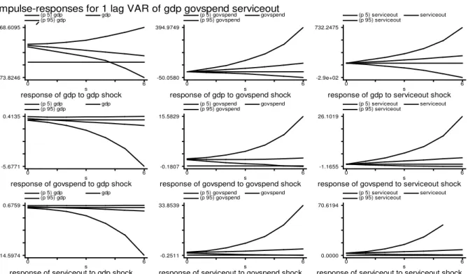
Persistence of shocks was found to have strong negative effects on life expectancy (depicting increases in inequality). Shock persistence was found to also have negative implications for the services and manufacturing sectors leading to contraction in output productivity from these sectors. Decreases in sectorial output will mean less capacity for sectors to create meaningful employment even though this may not suggest a high level of staff disengagement.

Table: 6 Forecast Error Variance Decomposition for the full Sample with Life expectancy Variance of life expectancy as explained by shocks in each variable

Full Sample Variables

t=2 t=3 t=4 t=6 t=8

GDP per capita 0.0003 0.0013 0.0023 0.0023 0.0023 Gov.spend 0.0674 0.0946 0.1218 0.1218 0.1218 Life. Exp. 0.9322 0.9042 0.8762 0.8762 0.8762

Table: 7 Forecast Error Variance Decomposition for the full Sample with Agricultural sector output Variance of agricultural output as explained by shocks in each variable

t=2 t=3 t=4 t=6 t=8

GDP per capita .0112 .0101 .0090 .0079 .0079 Gov. spend .0135 .0114 .0093 .0072 .0072 Agr. out .9746 .9784 .9862 .9940 .9940

Table: 8 Forecast Error Variance Decomposition for the full Sample with Service Sector Output Variance of services output as explained by shocks in each variable

t=2 t=3 t=4 t=6 t=8

GDP per capita .0548 .9999 1.4500 1.4500 1.4500 Gov. spend .1273 .1517 .1517 .1517 .1517 Ser. Out. .8178 .7484 .6792 .6792 .6792

(12)

Table: 9 Forecast Error Variance Decomposition for the full Sample with Manufacturing Sector Output Variance of life expectancy as explained by shocks in each variable

t=2 t=3 t=4 t=6 t=8

GDP per capita .8673 .8867 .8860 .8860 .8860 Gov. spend .1123 .1124 .1125 .1125 .1125 Man. out .0203 .0209 .0215 .0215 .0215

The response of government to shocks to GDP and fiscal spending in their decision to improve welfare were found to be interesting. It was observed that while decreases in welfare were noticeable and affected inequality in subsequent periods. Fiscal spending decreases were only noticeable initially. In subsequent periods governments probably adjusted budgets and sourced for alternative funds to finance infrastructural provision.

The variance decomposition for sectors yield that shocks to the manufacturing and services sectors affect output production for sectors. The negative effects of shocks to the agricultural sector are less; this is due to the informal nature of the sector.

Fig. 6 One lag impulse response function of life expectancy to shocks in GDP and government Spending

Source:ăAuthor’săcomputations

Impulse-responses for 1 lag VAR of gdp govspend lifeexp

Errors are 5% on each side generated by Monte-Carlo with 500 reps

response of gdp to gdp shock

s

(p 5) gdp gdp

(p 95) gdp

0 6

0.0000 82.0708

response of gdp to govspend shock

s

(p 5) govspend govspend (p 95) govspend

0 6

-53.5908 37.5235

response of gdp to lifeexp shock

s (p 5) lifeexp lifeexp (p 95) lifeexp

0 6

-7.6175 18.4078

response of govspend to gdp shock

s

(p 5) gdp gdp

(p 95) gdp

0 6

-0.4199 0.1167

response of govspend to govspend shock

s

0 6

0.0000 1.8643

response of govspend to lifeexp shock

0 6

-0.0952 0.2074

response of lifeexp to gdp shock

s

(p 5) gdp gdp

(p 95) gdp

0 6

-0.0747 0.0819

response of lifeexp to govspend shock

s

0 6

-0.2728 0.0580

response of lifeexp to lifeexp shock

0 6

(13)

Fig. 7 Two lag impulse response function of life expectancy to shocks in GDP and government Spending

Fig. 8 Three lag impulse response function of life expectancy to shocks in GDP and government Spending

s

(p 5) gdp gdp

(p 95) gdp

0 6

0.0000 171.3342

s

0 6

-42.5068 84.1455

response of gdp to lifeexp shock

0 6

-84.0683 104.5136

s

(p 5) gdp gdp

(p 95) gdp

0 6

-0.3995 0.6741

s

0 6

-0.1116 1.8414

response of govspend to lifeexp shock

0 6

-0.1899 0.9084

response of lifeexp to gdp shock

s

(p 5) gdp gdp

(p 95) gdp

0 6

0.0000 0.7025

response of lifeexp to govspend shock

s

0 6

-0.2731 0.3202

response of lifeexp to lifeexp shock

0 6

0.0000 1.1884

Errors are 5% on each side generated by Monte-Carlo with 500 reps response of gdp to gdp shocks

(p 5) gdp gdp (p 95) gdp

0 6

0.0000 133.6891

response of gdp to govspend shocks (p 5) govspend govspend (p 95) govspend

0 6

-46.1546 76.2956

response of gdp to lifeexp shocks (p 5) lifeexp lifeexp (p 95) lifeexp

0 6

-27.0678 38.2408

response of govspend to gdp shocks (p 5) gdp gdp (p 95) gdp

0 6

-0.4541 0.0892

response of govspend to govspend shocks (p 5) govspend govspend (p 95) govspend

0 6

0.0000 1.8351

response of govspend to lifeexp shocks (p 5) lifeexp lifeexp (p 95) lifeexp

0 6

-0.1004 0.3012

response of lifeexp to gdp shock s

0 6

-0.2491 0.0000

response of lifeexp to govspend shock s

0 6

-0.1885 0.0035

response of lifeexp to lifeexp shock s

(p 5) lifeexp lifeexp (p 95) lifeexp

0 6

(14)

Fig. 9 One lag impulse response function of agricultural output to shocks in GDP and government Spending

Fig. 10 Two lag impulse response function of agricultural output to shocks in GDP and government Spending

Source:ăAuthor’săComputations

Impulse-responses for 1 lag VAR of gdp govspend agricout

s

(p 5) gdp gdp

(p 95) gdp

0 6

0.0000 81.4469

s

0 6

-97.9948 68.0738

response of gdp to agricout shock

s (p 5) agricout agricout (p 95) agricout

0 6

-60.5092 14.6111

response of govspend to gdp shocks

(p 5) gdp gdp

(p 95) gdp

0 6

-0.5000 0.0423

response of govspend to govspend shocks

0 6

-0.1440 1.8410

response of govspend to agricout shocks

(p 5) agricout agricout (p 95) agricout

0 6

-1.3251 0.2303

response of agricout to gdp shock

s

(p 5) gdp gdp

(p 95) gdp

0 6

-0.7457 0.1242

response of agricout to govspend shock

s

0 6

-0.4676 2.2698

response of agricout to agricout shock

0 6

0.0000 5.2324

Impulse-responses for 2 lag VAR of gdp govspend agricout

Errors are 5% on each side generated by Monte-Carlo with 500 reps response of gdp to gdp shock

s (p 5) gdp gdp (p 95) gdp

0 6

0.0000 189.1404

s

0 6

-93.3262 169.5581

response of gdp to agricout shock

0 6

-49.0158 50.9712

0 6

-0.4497 0.0751

s

0 6

-0.3413 1.8392

response of govspend to agricout shock

0 6

-1.0571 0.2161

response of agricout to gdp shock

0 6

-0.8198 0.1617

response of agricout to govspend shock

s

0 6

-0.8107 1.5237

response of agricout to agricout shock

0 6

(15)

Fig. 11 Three lag impulse response function of agricultural output to shocks in GDP and government Spending

Fig. 12 One lag impulse response function of services output to shocks in GDP and government Spending

Source:ăAuthor’săComputations Impulse-responses for 3 lag VAR of gdp govspend agricout

0 6

0.0000 140.2077

0 6

-99.1230 132.3278

response of gdp to agricout shocks (p 5) agricout agricout (p 95) agricout

0 6

-43.5043 27.9700

0 6

-0.4631 0.0736

0 6

-0.0451 1.8051

response of govspend to agricout shocks (p 5) agricout agricout (p 95) agricout

0 6

-1.0185 0.2585

response of agricout to gdp shocks (p 5) gdp gdp (p 95) gdp

0 6

-0.7146 0.2030

response of agricout to govspend shocks (p 5) govspend govspend (p 95) govspend

0 6

-0.8499 1.4196

response of agricout to agricout shocks (p 5) agricout agricout (p 95) agricout

0 6

0.0000 3.5789

Impulse-responses for 1 lag VAR of gdp govspend serviceout

response of gdp to gdp shocks

(p 5) gdp gdp

(p 95) gdp

0 6

-73.8246 168.6095

response of gdp to govspend shocks

0 6

-50.0580 394.9749

response of gdp to serviceout shocks

(p 5) serviceout serviceout (p 95) serviceout

0 6

-2.9e+02 732.2475

s

(p 5) gdp gdp

(p 95) gdp

0 6

-5.6771 0.4135

s

0 6

-0.1807 15.5829

response of govspend to serviceout shock

s

0 6

-1.1655 26.1019

response of serviceout to gdp shock

s

(p 5) gdp gdp

(p 95) gdp

0 6

-14.5974 0.6759

response of serviceout to govspend shock

s

0 6

-0.2511 33.8539

response of serviceout to serviceout shock

s

0 6

(16)

Fig. 13 Two lag impulse response function of services output to shocks in GDP and government Spending

Fig. 14 Three lag impulse response function of services output to shocks in GDP and government Spending

Source: Authors Computations Impulse-responses for 2 lag VAR of gdp govspend serviceout

(p 5) gdp gdp

(p 95) gdp

0 6

-40.9541 426.3102

0 6

-1.1e+02 146.6459

0 6

-5.7e+02 298.5542

response of govspend to gdp shocks

(p 5) gdp gdp

(p 95) gdp

0 6

-6.6623 0.3571

response of govspend to govspend shocks

0 6

-0.0402 6.0610

response of govspend to serviceout shocks

0 6

-0.8868 14.4169

response of serviceout to gdp shocks

(p 5) gdp gdp

(p 95) gdp

0 6

-14.3325 0.3433

response of serviceout to govspend shocks

0 6

-0.7050 12.3517

response of serviceout to serviceout shocks

0 6

0.0000 32.9414

Impulse-responses for 3 lag VAR of gdp govspend serviceout

0 6

-12.0798 220.0564

0 6

-61.0811 97.1099

0 6

-2.9e+02 199.5521

0 6

-2.9852 0.3317

s

0 6

0.0000 4.3053

response of govspend to serviceout shock

s

0 6

-0.4921 8.1348

response of serviceout to gdp shock

0 6

-6.0200 0.3188

response of serviceout to govspend shock

s

0 6

-0.0837 7.3024

response of serviceout to serviceout shock

s

0 6

(17)

Fig. 15 One lag impulse response function of manufacturing output to shocks in GDP and government Spending

Source: Authors Computations

Fig. 16 Two lag impulse response function of manufacturing output to shocks in GDP and government Spending

Source: Authors Computations Impulse-responses for 1 lag VAR of gdp govspend manufactout

0 6

-5.5e+02 1.1e+03

0 6

-9.3e+02 1.7e+03

response of gdp to manufactout shocks (p 5) manufactout manufactout (p 95) manufactout

0 6

-3.6e+02 455.9106

0 6

-16.5605 51.1949

0 6

-24.7375 74.3240

response of govspend to manufactout shocks (p 5) manufactout manufactout (p 95) manufactout

0 6

-8.3630 24.7268

response of manufactout to gdp shocks (p 5) gdp gdp (p 95) gdp

0 6

-3.5093 11.2869

response of manufactout to govspend shocks (p 5) govspend govspend (p 95) govspend

0 6

-4.9909 16.3170

response of manufactout to manufactout shocks (p 5) manufactout manufactout (p 95) manufactout

0 6

-0.7939 6.4885

Impulse-responses for 2 lag VAR of gdp govspend manufactout

0 6

-6.2e+08 2.5e+10

0 6

-1.8e+08 8.6e+09

0 6

-4.9e+07 2.1e+09

0 6

-4.2e+07 1.1e+09

0 6

-1.4e+07 3.9e+08

0 6

-3.3e+06 9.7e+07

response of manufactout to gdp shocks (p 5) gdp gdp (p 95) gdp

0 6

-1.1e+07 4.7e+07

response of manufactout to govspend shocks (p 5) govspend govspend (p 95) govspend

0 6

-3.6e+06 1.6e+07

response of manufactout to manufactout shocks (p 5) manufactout manufactout (p 95) manufactout

0 6

(18)

Fig. 17 Three lag impulse response function of manufacturing output to shocks in GDP and government Spending

Source: Authors Computations

In providing answers to the study objectives we rely on the results outcomes:

 Although the effect of GDP shocks to life expectancy were not immediate, it was found to be transmitting reducing effects to life expectancy and increasing inequality in countries.

 Negative shocks were also exerted on sectorial output production for the services and manufacturing sectors although these did not have significant implications for manufacturing.

 Negative shocks were found to have weak implications for the services sector, this were not noticeable for the agricultural sector, these are two labour intensive sectors with significant implicative effects for employment.

Conclusion

In this section we conclude. Negative shocks to GDP were found to significantly increase inequality in countries particularly after the first periods. The same were observed for sectors although the results were only weakly significant for the services sector. The impulse response function of life expectancy to GDP and fiscal spending had strong negative implications for life expectancy. For sectors these were not immediately noticeable for the manufacturing and services sector outputs and no decreases were observed for the agricultural sector.

The shock to fiscal spending on life expectancy increased inequality after the first period and were found to frizzle out in the subsequent periods as government adapted to shocks, through budget adjustments.

GDP and fiscal shocks due to financial volatility were found to have negative impacts on life expectancy and also across sectors indicating that a high level of uncertainty due to financial friction can have strong consequences for inequality in Africa, although this effect was not significant for the manufacturing and agricultural sector outputs. In concluding, the assertion earlier made that a sector is not likely to affect GDP adversely particularly in economies with multiple sectors but that diminished social infrastructural provision due to reduction in government spending on social infrastructure, will mean poor FDI inflow which is likely to affect GDP appeared to be quite plausible, therefore improved capital inflow into the economy could act as a buffer for the effects of shocks from sectors to aggregate GDP.

Impulse-responses for 3 lag VAR of gdp govspend manufactout

0 6

-2.4e+05 4.5e+08

0 6

-7.9e+04 1.6e+08

0 6

-4.2e+04 8.0e+07

0 6

-5.4e+03 8.8e+06

0 6

-2.1e+03 3.0e+06

0 6

-8.1e+02 1.5e+06

response of manufactout to gdp shock s

0 6

-1.0e+05 4.0e+05

response of manufactout to govspend shock s

0 6

-3.7e+04 1.4e+05

response of manufactout to manufactout shock s

(p 5) manufactout manufactout (p 95) manufactout

0 6

(19)

Recommendation

In this subsection we make useful recommendation for policy purposes. It is necessary for government to provide basic social security blankets for people living below the poverty line in many African countries by making basic medical facilities more accessible and easily affordable particularly in rural communities to help reduce poverty and mortality rates in general, since it was discovered that GDP shocks to life expectancy was transmitting reducing effects to life expectancy and increasing inequality in countries.

Sectoral performances also show poor ability of labour intensive sector to withstand the negative shocks in GDP. Adequate attention should be paid to socio infrastructural challenges as this could reduce the transaction cost of private firm activity. Since government also seem to be the highest employer of labour in the services sector e.g. schools, hospitals, airports and other social services, encouragement of other sectors such as manufacturing and agriculture where such negative implicative job reducing effects are likely to occur should be boosted.

Finally effective use of government funds as an intervention mechanism particularly in short term sectoral improvements such as business information provision, reduction in business permits processing time and avoidance of multiple taxation could encourage private investment in the manufacturing and agricultural sectors

The Authors Express Thanks to Inesa Love for PVAR Codes, and express heartfelt gratitude to Gravier-Rymaszewska for making his paper available.

References

[1] Africa’să Pulseă 2014ă “Worldă Bankă ă Journală onă Economică Growth”ă Vol.ă 9ă Aprilă 2014ă Availableă on http://www.worldbank.org/

content/dam/Worldbank/document/Africa/Report/Africas-Pulse-brochure_Vol9.pdf

[2] Arellano,ă M.,ă andă Bond,ă S.ă (1991).ă ‘Someă testsă ofă specificationă foră panelă data:ă Monteă Carloă evidenceă andă ană applicationă toă employment

equations’.ăTheăReview of Economic Studies, 58(2): 277.

[3] Arellano,ăM.,ăandăBover,ăO.ă(1995).ă‘Anotherălookăatătheăinstrumentalăvariableăestimationăofăerror-componentsămodels’.ăJournalăofăEconometrics,ă

68(1): 29-51.

[4] Blundell,ăR.,ăandăBond,ăS.ă(1998).ă‘Initialăconditionsăandămomentărestrictionsăinădynamicăpanelădataămodels’.ăJournalăofăEconometrics,ă87(1):ă

115-43.

[5] Boschini,ăA.,ăandăOlofsgård,ăA.ă(2007).ă‘Foreignăaid:ăAnăinstrumentăforăfightingăcommunism?’.ăJournalăofăDevelopmentăStudies, 43(4): 622-48. [6] Breitung,ăJ.ă(2001).ă‘Theălocalăpowerăofăsomeăunitărootătestsăforăpanelădata’.ăBingley:ăEmeraldăGroupăPublishingăLtd.

[7] Canova, F. and M. Ciccarelli, (2004), Forecasting and turning point predictions in a Bayesian panel VAR model, Journal of Econometrics 120, 327-59

[8] Chong, A., and Gradstein,ăM.ă(2008).ă‘Whatădeterminesăforeignăaid?ăTheădonors’ăperspective’.ăJournalăofăDevelopmentăEconomics,ă87(1):ă1-13.

[9] Dang,ăH.,ăKnack,ăS.,ăandăRogers,ăF.ă(2009).ă‘Internationalăaidăandăfinancialăcrisesăinădonorăcountries’.ăPolicyăResearchăWorking Paper 5162.

Washington, DC: World Bank.

[10] Faini, R. (2006). Foreign aid and fiscal policy. London: Centre for Economic Policy Research.

[11] Frot,ă E.ă (2009).ă ‘Aidă andă financială crisis:ă shallă weă expectă developmentă aidă toă fall?’.ă Workingă Paper.ă Stockholm:ă Stockholmă School of

Economics.

[12] Hansen,ăH.,ăandăHeadey,ăD.D.ă(2010).ă‘Theăshort-runămacroeconomicăimpactăofăforeignăaidătoăsmallăstates:ăAnăagnosticătimeăseriesăanalysis’.ă

The Journal of Development Studies, 46(5): 877-96.

[13] Hansen,ăH.,ăandăTarp,ăF.ă(2001).ă‘Aidăandăgrowthăregressions’.ăJournalăofăDevelopmentăEconomics,ă64(2):ă547-70.

[14] Gravier-Rymaszewska(2012)ă“HowăAidăSupplyăRespondsătoăEconomicăCrisesăAăPanelăVARăApproach”ăUNUWIDERăWorkingăPaperăAvailableă

on http://www.wider.unu.edu/publications/working-papers/2012/en_GB/wp2012-025/

[15] Im,ăK.,ăPesaran,ăM.,ăandăShin,ăY.ă(2003).ă‘Testingăforăunitărootsăinăheterogeneousăpanels’.ăJournalăofăEconometrics,ă115(1):ă53-74. [16] Knack, S. (2001). Aid dependence and the quality of governance: Cross-country empirical tests. Southern Economic Journal, 68(2), 310–29.

[17] Kraay,ă Aartă (2004).ă “Whenă Isă Growthă Pro-Poor? Cross-Countryă Evidence”.ă IMFă Workingă Paperă Availableă onă

https://www.imf.org/external/pubs/ft/wp/2004/wp0447.pdf

[18] Laeven,ăL.,ăandăValencia,ăF.ă(2010).ă‘Resolutionăofăbankingăcrises:ăTheăgood,ătheăbad,ăandătheăugly’.ăWorkingăPaperă10:ă146.ăWashington,ăDC:ă

IMF.

[19] Levin,ăA.,ăLin,ăC.,ăandăJamesăChu,ăC.ă(2002).ă‘Unitărootătestsăinăpanelădata:ăasymptoticăandăfinite-sampleăproperties’.ăJournalăofăEconometrics,ă

108(1): 1-24.

[20] Ojeagaă(2012)ă“Economicăpolicy,ădoesăItăhelpălifeăexpectancy?ăAnăAfricanăEvidenceăofătheăRoleăofăEonomicăPolicyăonăLongevity.”ăAvailableăonă

https://mpra.ub.uni-muenchen.de/secure/40199/1/MPRA_paper_40199.pdf

[21] Rajan,ăR.,ăandăSubramanian,ăA.ă(2008).ă‘Aidăandăgrowth:ăWhatădoesăthe cross-countryăevidenceăreallyăshow?’.ăTheăReviewăofăEconomicsăandă

Statistics, 90(4): 643-65.

[22] Reinhart,ăC.,ăandăRogoff,ăK.ă(2008),ă‘Bankingăcrises:ăanăequalăopportunityămenace’.ăTechnicalăreport,ăCambridge,ăMass:ăNational Bureau of

Economic Research.

[23] World Bank Press Release 2012.