Increasing fMRI Sampling Rate Improves Granger
Causality Estimates
Fa-Hsuan Lin1,2*, Jyrki Ahveninen3, Tommi Raij3, Thomas Witzel3, Ying-Hua Chu1, Iiro P. Ja¨a¨skela¨inen2, Kevin Wen-Kai Tsai1,2, Wen-Jui Kuo4, John W. Belliveau3
1Institute of Biomedical Engineering, National Taiwan University, Taipei, Taiwan,2Department of Biomedical Engineering and Computational Science, Aalto University, Espoo, Finland,3Athinoula A. Martinos Center for Biomedical Imaging, Massachusetts General Hospital, Harvard Medical School, Boston, Massachusetts, United States of America,4Institute of Neuroscience, National Yang-Ming University, Taipei, Taiwan
Abstract
Estimation of causal interactions between brain areas is necessary for elucidating large-scale functional brain networks underlying behavior and cognition. Granger causality analysis of time series data can quantitatively estimate directional information flow between brain regions. Here, we show that such estimates are significantly improved when the temporal sampling rate of functional magnetic resonance imaging (fMRI) is increased 20-fold. Specifically, healthy volunteers performed a simple visuomotor task during blood oxygenation level dependent (BOLD) contrast based whole-head inverse imaging (InI). Granger causality analysis based on raw InI BOLD data sampled at 100-ms resolution detected the expected causal relations, whereas when the data were downsampled to the temporal resolution of 2 s typically used in echo-planar fMRI, the causality could not be detected. An additional control analysis, in which we SINC interpolated additional data points to the downsampled time series at 0.1-s intervals, confirmed that the improvements achieved with the real InI data were not explainable by the increased time-series length alone. We therefore conclude that the high-temporal resolution of InI improves the Granger causality connectivity analysis of the human brain.
Citation:Lin F-H, Ahveninen J, Raij T, Witzel T, Chu Y-H, et al. (2014) Increasing fMRI Sampling Rate Improves Granger Causality Estimates. PLoS ONE 9(6): e100319. doi:10.1371/journal.pone.0100319
Editor:Daniele Marinazzo, Universiteit Gent, Belgium
ReceivedDecember 29, 2013;AcceptedMay 26, 2014;PublishedJune 26, 2014
Copyright:ß2014 Lin et al. This is an open-access article distributed under the terms of the Creative Commons Attribution License, which permits unrestricted use, distribution, and reproduction in any medium, provided the original author and source are credited.
Funding:This work was supported by R01MH083744, R01HD040712, R01NS037462, R01NS048279 (National Institutes of Health), NSC 101-2628-B-002-005-MY3, NSC 100-2325-B-002-046 (National Science Council, Taiwan), 100-EC-17-A-19-S1-175 (Ministry of Economic Affairs, Taiwan), NHRI-EX102-10247EI (National Health Research Institute, Taiwan), and Academy of Finland (the FiDiPro program). The funders had no role in study design, data collection and analysis, decision to publish, or preparation of the manuscript.
Competing Interests:Authors Fa-Hsuan Lin and Jyrki Ahveninen are both Academic Editors of PLOS ONE. Others authors have declared that no competing interests exist. This does not alter the authors’ adherence to PLOS ONE policies on sharing data and materials.
* Email: [email protected]
Introduction
Determining causal mechanisms by which different brain areas interact to support cognition and behavior has been a persistent challenge in neuroscience. Whereas analyzing synchronization of cerebral activations can identify cortical areas acting in concert, revealing causal influences among them requires measures of effective connectivity[1–3]. Previously, effective connectivity analyses of human PET [4] and fMRI [5–8] data have been conducted using structural equation modeling (SEM), which aims at determining directional modulations across the activated areas using covariance or correlation matrices derived from the measured time series [9]. However, a major limitation of SEM is that it requires strong a prioriassumptions on the number and directionality of connections, which are often difficult to justify or validate. Similar limitations exist in dynamic causal modeling (DCM), which also requires a priori models of directional connections [10–12]. To circumvent such limitations, the tech-nique of Granger causality [13] has been applied to data obtained with both EEG [14–22] and fMRI [18,23–29]. The main advantage of Granger causality over SEM and DCM is that it can estimate the directionality of modulations within a network withouta prioriassumptions on which connections are active and on directions of the connections. Essentially, Granger causality
tests how additional information improves prediction of the future of a given time series. In other words, a Granger causal influence from a time series ‘‘X’’ to time-series ‘‘Y’’ exists if the combined information from ‘‘X’’ and ‘‘Y’’ predicts the future of ‘‘Y’’ better than information from ‘‘Y’’ alone.
Functional MRI of the human brain [30] with blood oxygenation level dependent (BOLD) contrast [31,32] is the prevailing method for studying brain functions noninvasively. There are two major limitations to using BOLD fMRI for causality modelling. First, BOLD signals are vascular responses that lag the underlying neuronal events by seconds [33] and may show notable voxel-to-voxel latency variability at the individual level [34]. However, it has been suggested that with appropriate modelling to obtain neuronal activity estimates, BOLD fMRI can still be used for causality modelling [35]. The other challenge for using BOLD fMRI in Granger causality estimation is the rather low sampling rate, which is critically important in all time series modeling. Typically fMRI Granger causality analyses use data sampled at the rate of approximately 1–2 s [24,26–29]. Such a slow sampling rate, which is necessary to achieve whole-brain fMRI coverage at a spatial resolution of 3–4 mm, provides only about 10–15 samples during the 20–30 sec duration of a canonical hemodynamic response function [36]. Estimating Granger
sality from fMRI time series recorded at such a low sampling rate can be problematic.
Using the recently developed dynamic functional magnetic resonance inverse imaging (InI), one can achieve an order of magnitude faster sampling rate. InI is based on the utilization of simultaneous measurements from multiple channels of an RF head coil array, and by solving sets of inverse problems InI can detect dynamic changes of the BOLD fMRI signals at,10 Hz sampling
rate with whole-brain coverage and approximately 5-mm spatial resolution at the cortex [37–39]. Our recent study suggests that, InI hemodynamic responses can elucidate neuronally related timing information when cross-subject and within-region variabil-ity is suppressed by averaging [40].
Several studies have consistently suggested that the sensitivity and stability of Granger causality values can be critically improved if the temporal sampling rate is high enough [26,41–47]. However, to our knowledge, there have been to date no studies empirically demonstrating this. Based on our data showing that the BOLD fMRI signal can reflect neuronal timing at the group level [40], here we hypothesize that increasing the fMRI sampling rate using InI one can provide more robust and sensitive Granger causality estimates compared to conventional multi-slice EPI acquisitions. We test this empirically using InI fMRI with 10-Hz InI sampling rate and a simple visuomotor detection task, which generates feed-forward inter-area information flow [48]. Three different time series were used in this study: fMRI raw time series, hemodynamic response function after General Linear Model, and the estimated neuronal activity using hemodynamic deconvolution. Time series with lower sampling rates (2 Hz, 1 Hz, 0.5 Hz, and 0.2 Hz) were artificially generated by either discarding InI samples or interpo-lating sub-sampled time series in order to keep the same number of time points. Our results indicate that the high sampling rate provided by InI can robustly improve detection of causal modulations between cortical areas.
Materials and Methods
Ethic statement, subjects, and tasks
This study was approved by the Institute Review Boards of National Taiwan University Hospital and National Yang Ming University. Written informed consent approved by the Institute Review Board of National Taiwan University Hospital and National Yang Ming University was obtained from each subject prior to participation. Healthy human volunteers (n= 23, 6 females, all right-handed, age 22–30 years) were presented with left or right visual hemifield reversing (8 Hz) checkerboard stimuli in a rapid event-related fMRI design. The hemifield checkerboard subtended a 4.3uvisual angle and was generated from 24 evenly distributed radial wedges and eight concentric rings of equal width. The stimuli were presented using the Psychtoolbox [49,50]. Stimulus duration was 500 ms; the onset of each presentation was randomized with a uniform distribution of inter-stimulus intervals varying from 3 to 16 s (average 10 s). Part of data has been previously reported in studying the correlation between hemody-namic and neuronal activity [51].
The subjects were instructed to press the button upon detecting a visual stimulus, presented randomly at the left or right side of the screen, with the hand ipsilateral to the stimulus. Thus, there were two conditions: right visual hemifield–right hand (R condition) and left visual hemifield–left hand (L condition). This relatively simple task was chosen for its feedforward connectivity from visual to motor systems. Accordingly, our a priori hypothesis predicted directional information flow from visual to motor cortices.
Twenty-four stimulation epochs were presented during four 240 s runs, resulting in a total of 96 trials per subject.
Structural MRI acquisitions and reconstructions
StructuralT1-weighted MRIs were acquired with a 3T scanner (Tim Trio, Siemens, Erlangen, Germany) and a 32-channel head phased array coil using a standard MPRAGE sequence (repetition time/echo time/inversion time [TR/TE/TI] = 2,530/3.49/ 1100 ms, flip angle = 7u, partition thickness = 1.33 mm, image matrix = 2566256, 128 partitions, field-of-view = 21 cm621 cm). The location of the gray-white matter boundary for each participant was estimated with an automatic segmentation algorithm to yield a triangulated mesh model with approximately 340,000 vertices [52–54]. This cortical model was then used to facilitate mapping of the structural image from native anatomical space to a standard cortical surface space [52,53]. Between-subjects averaging was done by morphing individual data through a spherical coordinate system [55].
fMRI inverse imaging (InI) acquisitions and reconstructions
BOLD-contrast fMRI data were acquired using inverse imaging [39,56], which included a reference scan to collect spatial information from different channels in a radio-frequency coil array and a set of dynamic scans to achieve high temporal sampling rate (.10 Hz) with whole brain coverage. The InI reference scan was collected using a single-slice echo-planar imaging (EPI) readout, after exciting one thick coronal slab covering the entire brain (FOV 256 mm6256 mm6256 mm;
64664664 image matrix) with the flip angle set to the gray matter
Ernst angle of 30u(considering the T1 of gray matter is 1 second at 3T). Partition phase encoding was used to obtain spatial information along the anterior-posterior axis (Y direction). EPI readout had frequency encoding along the superior-inferior (Z direction) and phase encoding along the left-right axis (X direction). We used TR = 100 ms, TE = 30 ms, band-width = 2604 Hz and a 12.8-s total acquisition time for the reference scan, allowing the coverage of the whole-brain volume with 64 partitions and two repetitions.
For the InI functional scans, we used the same volume prescription, TR, TE, flip angle, and bandwidth as for the InI reference scan. The principal difference was that, to achieve the high temporal resolution, partition phase encoding (in the Z direction) was removed so that the full volume was excited, and the spins were spatially encoded by a single-slice EPI trajectory, resulting in a coronal X/Z projection image with spatially collapsed projection along the anterior-posterior direction. The k-space InI reconstruction algorithm [57] was then used to estimate the spatial information along the anterior-posterior axis. In each run, we collected 2,400 measurements after collecting 32 measurements in order to reach the longitudinal magnetization equilibrium. A total of 4 runs of data were acquired from each participant. The total fMRI acquisition time for each subject was 16 minutes.
standard deviation of the time series during the 6-s pre-stimulus interval. Using these noise estimates, dynamic statistical paramet-ric maps (dSPMs) were derived as the time-point by time-point ratio between the InI reconstruction values and the baseline noise estimates. Such dSPMs can be assumed to betdistributed under the null hypothesis of no hemodynamic response [58].
Each subject’s InI time series, including the estimated hemo-dynamic responses and raw fMRI time series before GLM, were spatially registered into their cortical surface space by using a 12-parameter affine transformation between the volumetric InI reference scan and the MPRAGE anatomical space (FSL, http://www.fmrib.ox.ac.uk/fsl). The resulting spatial transforma-tion was subsequently applied to each time point of the reconstructed InI volume. For inter-subject averaging the individ-ual functional results were co-registered to a spherical brain surface representation [59].
Regions-of-interest (ROIs) were determined by the spatial distribution of the temporally averagetstatistics greater than 4.0 (Bonferroni corrected p-value,0.05) between 4 s and 7 s after visual stimulus onset. This interval was chosen to capture the maximum BOLD response. Time courses for each ROI were extracted and averaged within the ROI for each subject separately.
Echo-planar imaging (EPI) collection and analysis
We also collected EPI with 2 s TR in order to use empirical data to compare the detection sensitivity to causality modulation using InI data. The subjects were instructed to perform the same lateralized visuomotor task as that during the InI acquisitions. Data were collected from 13 subjects over one 4-minute run, where 30 left hemifield and 30 right hemifield visual stimulations were randomly presented. EPI parameters were: TR/TE = 2000/ 30 ms, field-of-view (FOV) = 2206220 mm, matrix = 64664, slice thickness = 4 mm, flip angle = 90u. For each subject, thirty-four trans-axial slices with no gap were acquired with the spatial coverage of cerebrum and cerebellum.
EPI fMRI data were first pre-processed for motion correction, slice timing correction, and spatial smoothing (12 mm 3D full-width-half-maximum Gaussian filter) by using the FreeSufer software (http://surfer.nmr.mgh.harvard.edu). We used GLM to identify visual and motor cortices with the FIR bases described above. Estimated hemodynamic activity from each subject was spatially registered to a common surface coordinate system using FreeSufer. The BOLD signals were then averaged across subjects and the dynamic significance of the BOLD signal was calculated using the dSPM procedure described above.
Time series preparation
In this study, we analyzed the causal modulation using the fMRI time series directly, instead of using the estimated HRF. In preparation of these fMRI time series, GLM was first used to identify the location of visual and sensorimotor cortices (see section fMRI inverse imaging (InI) acquisitions and reconstruc-tions and Echo-planar imaging (EPI) collection and analysis above). These time series were then averaged within each ROI from each subject. The DC value and the linear drift were also removed from these time series.
This study evaluates how the increased temporal resolution in InI acquisitions and reconstructions can help elucidate the causal interactions in the human visuomotor system. This was done by parametrically downsampling the InI data to generate time series from 0.1-s to 0.5, 1, and 2-s temporal resolution, the last of which is quite common in whole-head fMRI studies. In addition, to avoid the confound of different sampling rates and thus different lengths
of time series, we also generated SINC-interpolated time series from the sub-sampled time series such that all time series have the same length in the causality analysis. Finally, we also used EPI time series (before GLM) to estimate causality modulations in order to compare the results based on down-sampled InI data.
Granger causality and conditional Granger causality analysis
We used an auto-regressive (AR) model to implement the Granger causality modeling. Consider a zero-mean time series at the ‘‘destination node’’,y(t). Thepth-order AR model description of y(t) is:
y(t)~X
p
k~1
aky(t{k)z"y(t),t~1 n, ð1Þ
whereakare AR model coefficients, andey(t) is the residual time series of AR model fitting at the destination node.nis the total number of samples in the time series. Provided with the time series from a ‘‘source’’,x(t), we can model the bivariate time series ofx(t) andy(t) as:
y(t),x(t)
½ T~
Xp
k~1
Ak½y(t{k),x(t{k)Tz"y,x(t),"x,x(t)T,t~1 n ð
2Þ
where Ak’s are the AR model coefficient matrices, and [e y,x(t), ex,x(t)]T is the joint bivariate residual time series of AR model fitting at the destination node and source node. The Granger causality metric is
GCx?y~log
Xn
t~1
"2 y(t)
,
Xn
t~1
"2 y,x(t)
!
ð3Þ
Since the bivariate time series [y(t),x(t)]Tcontains the information of univariate time series y(t), from Cauchy inequality we can conclude thatGxRyis well defined and positive since the quotient inside the logarithm is greater or equal to one. Previously, it has been suggested that the inference ofGxRycan be calculated by referring ((n2p)/p) (exp(GxRy)–(n22p)/(n2p)) to an Fdistribution with (p,n22p) degrees of freedom [60].
For each pair of ROI time series (‘‘X’’ and ‘‘Y’’), we respectively calculated the Granger causality GxRy and GyRx. Previous simulation studies suggest that naive computation of Granger causality over fMRI signals can be misleading [26]. However, the influence difference (the difference between the pair GxRy and GyRx) can be much more robust [25,26]. Following this rationale, for each pair of ROIs, we only calculated the difference between two Granger causality values in order to identify the dominant influence direction.
The implementation of the AR modeling was done by the ARFIT algorithm [61,62], where the optimal model order was jointly determined by model fitting (i.e., favoring the model with smaller power of the residual time series after fitting) and model parsimoniousness (i.e., favoring a lower order model). This implementation has been previously used to explore the causal modulation of epileptic spike propagation measured by MEG [63]. Allowing the AR model ordering ranging between 1 and 20 or the largest order allowed by the number of sample, we used the Bayesian information criterion to choose the optimal order of the AR model. In the Granger causality analysis on time series of a Fast fMRI Improves Causality Estimates
pair of ROIs, we used the minimum of the estimated AR model orders to estimate the GC for the sake of model simplicity.
We used a non-parametric approach to estimate the statistical significance of the influence difference, because the null distribu-tion of such influence difference has no analytic form. Further-more, if we want to use the F/Chi-square distributions in causality estimation, samples in the time series need to be independent. This may not be the case in BOLD-contrast fMRI time series with different sampling rates. Our non-parametric analysis started from generating the null distribution of influence difference using the Adjusted Amplitude Fourier Transform (AAFT), a method of generating surrogate time series while preserving the linear correlation structure of the original time series and the marginal distribution [64]. The permutation procedure was repeated 1000 times for Granger causality analysis and 100 times for conditional Granger causality analysis, because the latter analysis took a longer computation time. We defined the p-value as the number of occurrences of the Granger causality values using a swapped source time series exceeding the Granger causality value using the original source time series. Thep-value of the Granger causality
difference in the group analysis was calculated accordingly as the ratio between the number of the Granger causality difference values from permuted time series higher than that from the original time series in each subject and the total number of permutation test across subjects. Note that such a p-value calculation amounts to a fixed-effect analysis.
Granger causality can be complicated by a ‘‘common source’’ problem. Specifically, the causal modulation between a pair of time series can be mediated through other time series within the set of analyzed time series. This problem has been partially addressed by the conditional Granger causality approach [25,65– 67]. In the case of studying the causal modulations between the time series pair [y(t), x(t)]T
, suppose that a multivariate auto-regressive model can be used to describe all other time series [z(t)]T. The conditional Granger causality cG
xRyis calculated as the ratio between the residual variance in the joint time series [y(t), z(t)]Tand the residual variance in the joint time series [x(t),y(t), z(t)]T
:
Table 1.Timing indices and the full-width-half-maximum (FHWM) of the group-average hemodynamic responses in five regions-of-interest.
V PCC PreM S M
Onset (s) L 0.63 0.91 0.69 1.04 1.18
R 0.60 1.03 0.84 1.04 1.19
Time-to-half (s) L 1.70 1.90 1.90 2.20 2.40
R 1.70 2.00 2.20 2.20 2.40
Time-to-peak (s) L 3.60 3.70 4.00 4.10 4.50
R 3.70 4.10 4.20 4.20 4.40
FWHM (s) L 4.60 4.30 5.10 4.60 4.70
R 4.80 4.80 4.70 4.60 4.60
V: visual cortex; PCC: parietal cortex; PreM: pre-motor cortex; S: sensorimotor cortex; M: motor cortex. L: left hemisphere (R condition). R: right hemisphere (L condition). doi:10.1371/journal.pone.0100319.t001
y(t),z(t)
½ T~
X
p
k~1
Bk½y(t{k),z(t{k)Tz"y,z(t),"z,y(t)T,t~1 n
x(t),y(t),z(t)
½ T~
X
p
k~1
Ck½x(t{k),y(t{k),z(t{k)Tz"x,yz(t),"y,xz(t),"z,xy(t)T,
t~1 n cGCx?y~log
Xn
t~1
"2 y,z(t)
,
Xn
t~1
"2 y,xz(t)
!
ð4Þ
Heuristically, conditional Granger causality evaluates the improve-ment of the additionally explained variance in the target time series by adding the source time series after controlling the information in all other time series. Statistical significance can be similarly derived from the empirical null distribution.
All calculations were done using Matlab (Mathworks, Natick, MA, USA).
Results
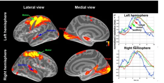
The visuomotor task elicited strongest BOLD signal at the left hemisphere, contralateral to the visual stimulus/motor response. Thus, results for the L condition are reported in the right hemisphere and the R condition in the left hemisphere. We identified five regions-of-interest (ROIs), including visual cortex (V), parietal cortex (PPC), pre-motor cortex (PreM), somatosen-sory cortex (S), and motor cortex (M) for both L and R conditions, as shown inFigure 1. Notably, the details of the average time courses (Figure 1) show sequential BOLD activity with different onsets, time-to-half (TTH), time-to-peak (TTP) timing, and width of regional hemodynamic response (Table 1).
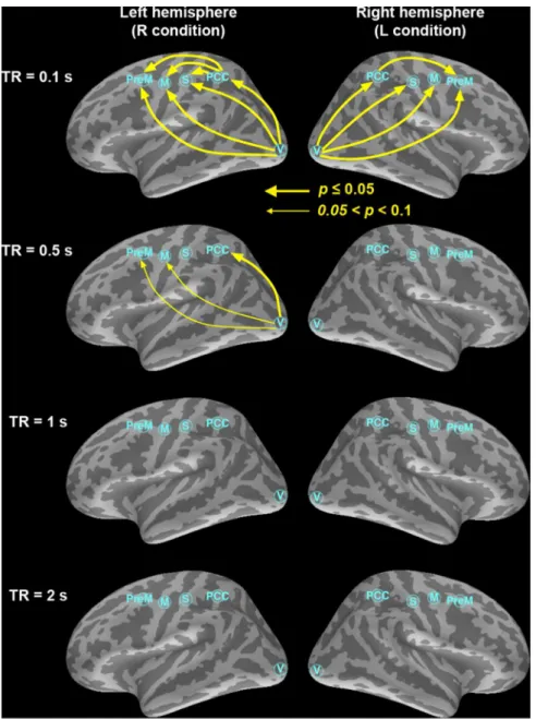
Figure 2. shows that increasing the fMRI sampling rate significantly improved the sensitivity of our Granger causality estimates, as indicated by the emergence of multiple directional influences consistent with the visuomotor task. The dominant direction of information flow between any two ROIs (denoted X and Y) was determined by calculating the difference (GXRY–
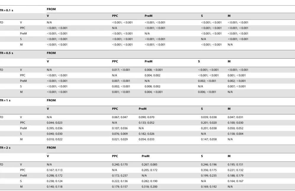
GYRX) between the two uni-directional Granger causality estimates [23,26]. Table 2 lists the order of the optimal AR model for each ROI time series. P-values of all directions of information flow between ROI’s were listed inTable 3. At the highest temporal resolution (TR = 0.1 s), significant bottom-up causal influences were observed from visual to PPC, premotor, somatosensory, and motor cortices in both left and right hemispheres. Reducing the temporal resolution clearly decreased the number of significant causality influences. At TR = 0.5 s, left hemisphere still shows three strong feedforward connections. However, the significance levels of two connections (from visual cortex to premotor and motor cortices) have decreased. Further lowering the sampling rate down to 1 s and 2 s, the conventional TR for whole-head EPI, shows no significant feedforward connections. In addition to the influence differences, we also report the Granger causality values and their associated signifi-cance inTable 4, showing that almost all causality estimates were significant at TR,= 1 s and non-significant at TR = 2 s and that the majority of statistically significant GC connections were bidirectional.
Granger estimates can be confounded by one source driving multiple targets. To reduce confounds related to potential common sources, we also calculated the difference conditional Granger causality values among pairs of the time series in 5 ROIs. Different from the Granger causality, conditional Granger causality estimates the specific information flow between two chosen ROIs while the information from all other ROIs through direct or indirect information flow are removed [65,67,68]. P-values are marginally different between Granger causality analysis and conditional Granger causality analysis in all sampling rates (Table 5). Again, increasing the TR gradually reduced the number of significant paths – no significant causal modulation was observed in both hemispheres at TR = 1 s and 2 s.
To confirm that the increased sensitivity in detecting feedfor-ward connections is not due to different time series length, we SINC interpolated the time series from the subsampled data such that all time series had the same length before Granger causality analysis. For example, TR = 0.5 s data were first down-sampled by 5-fold from the densely sampled time series with TR = 0.1 s and subsequently SINC interpolated by 5-fold. Results inFigure 3 shows that, while interpolation can artificially help improve the detection, slow sampling rates at the order of 1 s cannot provide significant feedforward connection estimates in left and right hemispheres. Specifically, we found that the significance levels for the VRM and VRPreM connections in the left hemisphere Table 2.The optimal order of the AR model of the time series at five ROI’s.
V PCC PreM S M
TR = 0.1 s L 11 11 11 11 12
R 10 8 9 9 9
TR = 0.5 s L 3 3 3 3 3
R 4 3 4 4 4
TR = 1 s L 1 1 2 1 1
R 2 2 2 2 2
TR = 2 s L 1 1 1 1 1
R 1 1 1 1 1
V: visual cortex; PCC: parietal cortex; PreM: pre-motor cortex; S: sensorimotor cortex; M: motor cortex. L: left hemisphere (R condition). R: right hemisphere (L condition). doi:10.1371/journal.pone.0100319.t002
Fast fMRI Improves Causality Estimates
decreased (increased p-value) at TR = 0.5 s. A significant VRPreM connection shows up at TR = 0.5 s in the right hemisphere after data interpolation. Results with TR = 1 s suggested possible VRPreM and VRM connections. However, the trend of losing detecting feedforward connections at a slower sampling rate prevails. In particularly, TR = 2 s, the typical whole-head EPI sampling rate, shows no significant connections in both hemispheres.
Finally, in addition to using down-sampled InI data, we also used EPI data with TR = 2 s record the subjects’s BOLD signal at visual and motor cortices in the same lateralized visuomotor task. Consistent with the down-sampled InI simulations (Table 3), we found that there was no significant VRM causal modulation in both R and L conditions (p-values = 0.27 and 0.22 for R and L conditions, respectively).
Discussion
Our results demonstrate that the inverse imaging method with a 20-fold increase in fMRI temporal resolution can greatly improve the detection power of causality analysis in the human brain. Using whole-head InI acquisitions with 100 ms temporal resolu-tion, we were able to infer directional causal influences between five functional areas activated during a lateralized visuomotor task in each hemisphere with both Granger causality and conditional Granger causality analyses. Consistent with thea priori predicted pattern of functional connectivity in a visuomotor choice-reaction task [48], the results were dominated by feedforward influences from visual to sensorimotor, premotor, and posterior parietal regions. These observations strongly underline the importance of high temporal sampling rates in determining effective connectivity, because the connectivity patterns only emerged at the 100 ms TR Table 3.P-values of all directions of information flow estimated by Granger causality between ROI’s at different sampling rates from 1000 bootstrap iterations.
TR = 0.1 s FROM
V PPC PreM S M
TO V N/A 1-p; 1-p 1-p; 1-p 1-p; 1-p 1-p; 1-p
PPC ,0.001; 0.006 N/A 1-p; 1-p 1-p; 1-p 1-p; 1-p
PreM ,0.001;,0.001 ,0.001; 0.006 N/A 1-p; 1-p 1-p; 1-p
S ,0.001; 0.016 0.002; 0.576 0.883; 0.897 N/A 1-p; 1-p
M ,0.001; 0.003 ,0.001; 0.390 0.110; 0.861 0.904; 0.256 N/A
TR = 0.5 s FROM
V PPC PreM S M
TO V N/A 1-p; 1-p 1-p; 1-p 1-p; 1-p 1-p; 1-p
PPC 0.027; 0.573 N/A 1-p; 1-p 1-p; 1-p 1-p; 1-p
PreM 0.069; 0.259 0.305; 0.618 N/A 1-p; 1-p 1-p; 1-p
S 0.120; 0.358 0.597; 0.152 0.891; 0.416 N/A 1-p; 1-p
M 0.076; 0.541 0.378; 0.128 0.489; 0.387 0.304; 0.470 N/A
TR = 1 s FROM
V PPC PreM S M
TO V N/A 1-p; 1-p 1-p; 1-p 1-p; 1-p 1-p; 1-p
PPC 0.377; 0.542 N/A 1-p; 1-p 1-p; 1-p 1-p; 1-p
PreM 0.119; 0.648 0.339; 0.540 N/A 1-p; 1-p 1-p; 1-p
S 0.224; 0.442 0.263; 0.324 0.551; 0.518 N/A 1-p; 1-p
M 0.206; 0.381 0.268; 0.280 0.374; 0.419 0.402; 0.426 N/A
TR = 2 s FROM
V PPC PreM S M
TO V N/A 1-p; 1-p 1-p; 1-p 1-p; 1-p 1-p; 1-p
PPC 0.744; 0.280 N/A 1-p; 1-p 1-p; 1-p 1-p; 1-p
PreM 0.669; 0.806 0.463; 0.833 N/A 1-p; 1-p 1-p; 1-p
S 0.713; 0.338 0.313; 0.610 0.636; 0.381 N/A 1-p; 1-p
M 0.668; 0.356 0.252; 0.543 0.602; 0.396 0.389; 0.382 N/A
Each cell contains twop-values. The leftp-value is for the left hemisphere (R condition) and the rightp-value is for the right hemisphere (L condition). Only lower-triangular off-diagonal entries are listed. Upper-lower-triangular off-diagonal entries can be calculated by (1–listedp-value). V: visual cortex; PCC: parietal cortex; PreM: pre-motor cortex; S: sensoripre-motor cortex; M: pre-motor cortex. L: left hemisphere (R condition). R: right hemisphere (L condition).
Table 4.P-values of Granger causality values between ROI’s at different sampling rates.
TR = 0.1 s FROM
V PPC PreM S M
TO V N/A ,0.001;,0.001 ,0.001;,0.001 ,0.001;,0.001 ,0.001;,0.001
PPC ,0.001;,0.001 N/A ,0.001;,0.001 ,0.001;,0.001 ,0.001;,0.001
PreM ,0.001;,0.001 ,0.001;,0.001 N/A ,0.001;,0.001 ,0.001;,0.001
S ,0.001;,0.001 ,0.001;,0.001 ,0.001;,0.001 N/A ,0.001;,0.001
M ,0.001;,0.001 ,0.001;,0.001 ,0.001;,0.001 ,0.001;,0.001 N/A
TR = 0.5 s FROM
V PPC PreM S M
TO V N/A 0.017;,0.001 0.008;,0.001 ,0.001;,0.001 ,0.001;,0.001
PPC ,0.001;,0.001 N/A 0.004; 0.002 ,0.001;,0.001 0.001;,0.001
PreM ,0.001;,0.001 0.007;,0.001 N/A 0.002;,0.001 0.002;,0.001
S ,0.001;,0.001 0.002;,0.001 0.008; 0.002 N/A 0.007;,0.001
M ,0.001;,0.001 0.001;,0.001 0.004;,0.001 0.006;,0.001 N/A
TR = 1 s FROM
V PPC PreM S M
TO V N/A 0.067; 0.047 0.090; 0.070 0.039; 0.038 0.047; 0.031
PPC 0.044; 0.023 N/A 0.133; 0.052 0.201; 0.020 0.100; 0.030
PreM 0.395; 0.036 0.107; 0.036 N/A 0.201; 0.038 0.050; 0.052
S 0.040; 0.030 0.076; 0.009 0.182; 0.026 N/A 0.158; 0.004
M 0.010; 0.022 0.021; 0.029 0.054; 0.033 0.147; 0.058 N/A
TR = 2 s FROM
V PPC PreM S M
TO V N/A 0.240; 0.170 0.267; 0.085 0.246; 0.196 0.195; 0.151
PPC 0.167; 0.113 N/A 0.205; 0.172 0.356; 0.175 0.221; 0.132
PreM 0.298; 0.172 0.172; 0.237 N/A 0.199; 0.235 0.188; 0.179
S 0.238; 0.124 0.222; 0.136 0.282; 0.190 N/A 0.164; 0.167
M 0.140; 0.118 0.179; 0.157 0.318; 0.200 0.169; 0.192 N/A
Each cell contains twop-values. The leftp-value is for the left hemisphere (R condition) and the rightp-value is for the right hemisphere (L condition). V: visual cortex; PCC: parietal cortex; PreM: pre-motor cortex; S: sensorimotor cortex; M: motor cortex. L: left hemisphere (R condition). R: right hemisphere (L condition).
doi:10.1371/journal.pone.0100319.t004
Fast
fMRI
Improves
Causality
Estimates
PLOS
ONE
|
www.ploson
e.org
7
June
2014
|
Volume
9
|
Issue
6
|
(Figures 2 and 3). Controlling the number of time points by interpolating the time series with a lower sampling rate can only partially mitigate the problem of losing sensitivity in correct causality estimates (Figure 3).
The advantage of higher temporal resolution has been suggested by simulation studies [26,41–46], but has not been previously shown with empirical data. Moreover, the previous simulation studies assumed that regular EPI would be used, where any increase in fMRI temporal resolution has to be traded off for smaller spatial coverage, poorer spatial resolution, or jittered designs that greatly increase the duration of the imaging session [2,69]. Specifically, limited by the gradient slew rate, the acquisition of each echo-planar imaging slice takes approximately 80 ms at ,3 mm63 mm spatial resolution. Assuming that 30
slices would be needed to cover the entire brain, a jittered stimulus
design would require a 30-fold increase in data acquisition time, leading to impractical session durations (several hours). With the InI approach in the present study, we obtained a whole-head volume in 100 ms, but it is possible to speed up the acquisition even further. The temporal resolution of InI is determined by TE (30 ms) optimized for the BOLD contrast and desired field-of-view/spatial resolution. Using partial Fourier acquisition and a higher readout bandwidth, the readout time could be reduced from 32 ms (2 KHz bandwidth and 64 lines) to 16 ms (6/8 partial Fourier, 48 lines at 3 KHz bandwidth) at the cost of reduced SNR. However, if using an echo-shifting pulse sequence [56,70], it is possible to achieve 20 ms TR at 30 ms TE. These future developments could allow for testing causal modulations between hemodynamic time series with putative latency differences well below 100 ms.
Figure 2. The dominant information flow calculated from the difference between two uni-directional Granger estimates among the visual (V), PPC, premotor (PreM), somatosensory (S), and motor (M) cortex ROIs at TR = 0.1 s, 0.5 s, 1 s, and 2 s.Significant causal modulations (p#0.05) were shown in thick yellow arrows and connections showing a trend of causal modulation (0.05,p#0.1) were shown in thin yellow arrows.
In this study we chose InI for its whole-brain coverage, reasonable spatial resolution at cortex, and high sampling rate (TR = 0.1 s). Note that recently there are other fast fMRI acquisition methods, such as generalized InI [71], fast fMRI [72], MR-encephalography (MREG) [73], and simultaneous multi-slice EPI [74] methods. Each method has different magnetization excitation strategies and image reconstruction algorithms. Yet all of them can provide a sub-second sampling rate. As we demonstrate that fast fMRI acquisitions can help improve detecting causal modulations in human brain in general, researchers can choose any method adaptively under different theoretical or practical concerns without losing the detection power.
InI trades off a small amount of spatial resolution in one encoding direction for a substantially higher temporal resolution.
Depending on the reconstruction methods, InI has approximately 5 mm spatial resolution at cortex using a 32-channel head coil array at 3T [37–39], which is in the range of spatial filtering/ smoothing that is typically applied in echo-planar imaging as a post-processing step. Without reaching the limit based on the electromagnetic theory [75,76], using a head coil array of more channels at a higher field (for example, 7T) could further improve the spatial resolution of InI. Novel reconstruction methods targeted at suppressing the point spread function, such as using the minimum L-1 norm constraint [77], can also be used to improve the spatial resolution in studies where the highest possible spatial resolution is critical.
In addition to the neurophysiologically expected feedforward modulation from VRPPCRpreMRM, our InI results also suggest direct feed-forward connectivity from V to preM, M, Table 5.P-values of all directions of information flow estimated by conditional Granger causality between ROI’s at different sampling rates from 100 bootstrap iterations.
TR = 0.1 s FROM
V PPC PreM S M
TO V N/A 1-p; 1-p 1-p; 1-p 1-p; 1-p 1-p; 1-p
PPC ,0.01; 0.01 N/A 1-p; 1-p 1-p; 1-p 1-p; 1-p
PreM ,0.01;,0.01 ,0.01; 0.01 N/A 1-p; 1-p 1-p; 1-p
S ,0.01;,0.01 ,0.01; 0.57 0.88; 0.89 N/A 1-p; 1-p
M ,0.01;,0.01 ,0.01; 0.37 0.11; 0.87 0.89; 0.26 N/A
TR = 0.5 s FROM
V PPC PreM S M
TO V N/A 1-p; 1-p 1-p; 1-p 1-p; 1-p 1-p; 1-p
PPC 0.03; 0.54 N/A 1-p; 1-p 1-p; 1-p 1-p; 1-p
PreM 0.07; 0.28 0.30; 0.62 N/A 1-p; 1-p 1-p; 1-p
S 0.10; 0.38 0.69; 0.15 0.88; 0.40 N/A 1-p; 1-p
M 0.08; 0.57 0.41; 0.13 0.49; 0.38 0.22; 0.48 N/A
TR = 1 s FROM
V PPC PreM S M
TO V N/A 1-p; 1-p 1-p; 1-p 1-p; 1-p 1-p; 1-p
PPC 0.37; 0.57 N/A 1-p; 1-p 1-p; 1-p 1-p; 1-p
PreM 0.13; 0.64 0.35; 0.54 N/A 1-p; 1-p 1-p; 1-p
S 0.20; 0.50 0.27; 0.32 0.56; 0.49 N/A 1-p; 1-p
M 0.22; 0.45 0.29; 0.29 0.36; 0.40 0.38; 0.43 N/A
TR = 2 s FROM
V PPC PreM S M
TO V N/A 1-p; 1-p 1-p; 1-p 1-p; 1-p 1-p; 1-p
PPC 0.73; 0.25 N/A 1-p; 1-p 1-p; 1-p 1-p; 1-p
PreM 0.67; 0.78 0.49; 0.84 N/A 1-p; 1-p 1-p; 1-p
S 0.70; 0.33 0.34; 0.64 0.66; 0.39 N/A 1-p; 1-p
M 0.65; 0.39 0.27; 0.56 0.58; 0.38 0.37; 0.39 N/A
Each cell contains twop-values. The leftp-value is for the left hemisphere (R condition) and the rightp-value is for the right hemisphere (L condition). Only lower-triangular off-diagonal entries are listed. Upper-lower-triangular off-diagonal entries can be calculated by (1–listedp-value). V: visual cortex; PCC: parietal cortex; PreM: pre-motor cortex; S: sensoripre-motor cortex; M: pre-motor cortex. L: left hemisphere (R condition). R: right hemisphere (L condition).
doi:10.1371/journal.pone.0100319.t005
Fast fMRI Improves Causality Estimates
and S. Although these influences can be supported by animal models showing direct structural connections from visual to sensory and motor cortices in rats [78], it is also possible that different neurovascular coupling in the different ROIs caused smearing of neuronal temporal information that reduced the sensitivity of GC to detect the dominant feedforward connections in our estimates.
In contrast to the present finding, previous studies have shown that EPI data may show causal modulation in the human sensorimotor system using EPI with TR in the order of 2 s [24,26]. However, this seeming discrepancy may be explained by the different nature of the present two-choice reaction-time task
and those used in many previous studies. Here, the group average reaction time was less than 400 ms [40]. Therefore, without considering the differential vascular responses at visual and sensorimotor cortices, the BOLD signal time series in the visual and sensorimotor cortices were expected to be delayed by only a few hundreds of milliseconds. Such a latency is difficult to be resolved by regular EPI with TR = 2 s. Consequently, one can expect that quite similar BOLD signal time series in visual and sensorimotor cortices were elicited during this task. Two similar time series are actually difficult to use Granger causality analysis to reveal any causal modulation between them. In a simple theoretical example with twoidentical time series, it is clear that
Figure 3. The dominant information flow calculated from the difference between two uni-directional Granger estimates among the visual (V), PPC, premotor (PreM), somatosensory (S), and motor (M) cortex ROIs at TR = 0.1 s, 0.5 s, 1 s, and 2 s.The time series at 0.5 s, 1 s, and 2 s were SINC interpolated such that all time series are of the same length as the 0.1 s time series, which contains the real measured data. Significant causal modulations (p#0.05) were shown in thick yellow arrows and connections showing a trend of causal modulation (0.05,p#0.1) were shown in thin yellow arrows. Importantly, only very little improvement is observed in the estimates where the number of observations is artificially increased using the SINC interpolation procedure: the strongest connectivity patterns are, clearly, observed in the 0.1-s condition with only real data.
the residual time series in modeling one time series will not be further improved by providing the other time series, because all information has been provided by the first time series already. In such a case, the Granger causality value will be insignificant becausenofurther reduction on the power of residual time series after modeling the first one.
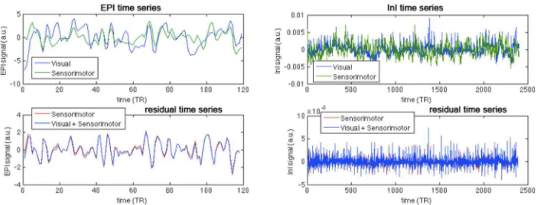
To support our argument above,Figure 4shows an example of two highly correlating (r= 0.446) EPI time series at visual and sensorimotor cortices from one representative subject.Figure 4 also shows the residual time series after modeling the sensorimotor time series when either only the sensorimotor cortex time series was provided, or both the sensorimotor and visual cortices time series were provided. The residual time series power only changed marginally (108.0R105.6; 2.3% reduction), in line with our main result of no significant Granger causality modulation between visual and sensorimotor cortices as measured by EPI with TR = 2 s. For comparison, we also show the InI time series in visual and sensorimotor cortices from one representative subject, and the residual time series after modeling the sensorimotor time series when either only the sensorimotor cortex time series was provided, or both the sensorimotor and visual cortices time series were provided. Visually, it is difficult to discern the precedence of either time series. However, numerically the variance of residual time series at the sensorimotor cortex was apparently reduced when the visual cortex time series was provided (0.0026R0.0023; 11.5% reduction).
Finally, it should be noted that BOLD-contrast fMRI measures the vascular responses secondary to neuronal events. On top of information reflecting neuronal activity, there are well document-ed vascular confounds in fMRI time series [34,79]. Our previous
study has shown that, with group averaging and improved sampling rate, inter-regional hemodynamic responses can be significantly correlated with inter-regional neuronal activity [51]. In this study, we chose a relatively simple two-choice reaction-time task with a priori assumption of observing strong feed-forward connectivity from the visual to the motor cortices. Such findings are consistent with a previous study [80] suggesting that fast sampling can eliminate confounding effects of differential HRF delays over areas by fine features of the HRF waveform (see also Table 1). However, while our results suggest that it is feasible to increase the fMRI sampling rate to enhance sensitive of causality estimates, caution must be always exercised when interpreting the results provided by these methods in the context of tasks eliciting more complex feed-forward/feedback information flow patterns.
Taken together, our results suggest that using MR InI with a 100 ms sampling interval (20-fold faster than conventional EPI), the sensitivity of detecting causal connectivity is significantly improved. We expect that this method can be used in other fMRI experiments to reveal effective connectivity when the vascular confound of the BOLD-contrast fMRI is carefully controlled and thus potentially open up entirely new possibilities for non-invasive imaging of effective connectivity in the human brain.
Author Contributions
Conceived and designed the experiments: FHL JA TR IPJ JWB. Performed the experiments: YHC KWT WJK. Analyzed the data: FHL. Contributed reagents/materials/analysis tools: TW YHC. Wrote the paper: FHL JA TR IPJ.
References
1. Cabeza R, McIntosh AR, Tulving E, Nyberg L, Grady CL (1997) Age-related differences in effective neural connectivity during encoding and recall. Neuroreport 8: 3479–3483.
2. Friston KJ (2007) Statistical parametric mapping: the analysis of funtional brain images. Amsterdam; Boston: Elsevier/Academic Press. vii, 647 p.
3. Friston KJ, Buechel C, Fink GR, Morris J, Rolls E, et al. (1997) Psychophysiological and modulatory interactions in neuroimaging. Neuroimage
6: 218–229.
4. McIntosh AR, Grady CL, Ungerleider LG, Haxby JV, Rapoport SI, et al. (1994) Network analysis of cortical visual pathways mapped with PET. J Neurosci 14: 655–666.
5. Buchel C, Friston KJ (1997) Modulation of connectivity in visual pathways by attention: cortical interactions evaluated with structural equation modelling and fMRI. Cereb Cortex 7: 768–778.
6. Buchel C, Coull JT, Friston KJ (1999) The predictive value of changes in effective connectivity for human learning. Science 283: 1538–1541.
7. McIntosh AR, Grady CL, Haxby JV, Ungerleider LG, Horwitz B (1996) Changes in limbic and prefrontal functional interactions in a working memory task for faces. Cereb Cortex 6: 571–584.
8. Friston KJ, Buchel C (2000) Attentional modulation of effective connectivity from V2 to V5/MT in humans. Proc Natl Acad Sci U S A 97: 7591–7596. 9. McArdle JJ, McDonald RP (1984) Some algebraic properties of the Reticular
Action Model for moment structures. Br J Math Stat Psychol 37 (Pt 2): 234–251. 10. Friston K (2009) Dynamic causal modeling and Granger causality Comments on: The identification of interacting networks in the brain using fMRI: Model selection, causality and deconvolution. Neuroimage.
11. Penny WD, Stephan KE, Mechelli A, Friston KJ (2004) Comparing dynamic causal models. Neuroimage 22: 1157–1172.
12. Friston KJ, Harrison L, Penny W (2003) Dynamic causal modelling. Neuro-image 19: 1273–1302.
13. Granger CWJ (1969) Investigating causal relations by econometric models and cross-Spectral methods. Econometrica 37: 424–438.
Figure 4. The EPI (left column) and InI (right column) time series at the visual and sensorimotor cortices from a representative subject (top panel) and the residual EPI (left column) and InI (right column) time series at the sensorimotor cortex after AR modeling using the sensorimotor cortex time series alone and both sensorimotor and visual cortices (bottom panel).
doi:10.1371/journal.pone.0100319.g004
Fast fMRI Improves Causality Estimates
14. Astolfi L, Cincotti F, Mattia D, Salinari S, Babiloni C, et al. (2004) Estimation of the effective and functional human cortical connectivity with structural equation modeling and directed transfer function applied to high-resolution EEG. Magn Reson Imaging 22: 1457–1470.
15. Blinowska KJ, Kus R, Kaminski M (2004) Granger causality and information flow in multivariate processes. Phys Rev E Stat Nonlin Soft Matter Phys 70: 050902.
16. Brovelli A, Ding M, Ledberg A, Chen Y, Nakamura R, et al. (2004) Beta oscillations in a large-scale sensorimotor cortical network: directional influences revealed by Granger causality. Proc Natl Acad Sci U S A 101: 9849–9854. 17. Chavez M, Martinerie J, Le Van Quyen M (2003) Statistical assessment of
nonlinear causality: application to epileptic EEG signals. J Neurosci Methods 124: 113–128.
18. Eichler M (2005) A graphical approach for evaluating effective connectivity in neural systems. Philos Trans R Soc Lond B Biol Sci 360: 953–967. 19. Hesse W, Moller E, Arnold M, Schack B (2003) The use of time-variant EEG
Granger causality for inspecting directed interdependencies of neural assemblies. J Neurosci Methods 124: 27–44.
20. Kaminski M, Ding M, Truccolo WA, Bressler SL (2001) Evaluating causal relations in neural systems: granger causality, directed transfer function and statistical assessment of significance. Biol Cybern 85: 145–157.
21. Kus R, Kaminski M, Blinowska KJ (2004) Determination of EEG activity propagation: pair-wise versus multichannel estimate. IEEE Trans Biomed Eng 51: 1501–1510.
22. Valdes-Sosa PA (2004) Spatio-temporal autoregressive models defined over brain manifolds. Neuroinformatics 2: 239–250.
23. Deshpande G, Sathian K, Hu X (2009) Effect of hemodynamic variability on Granger causality analysis of fMRI. Neuroimage 52: 884–896.
24. Goebel R, Roebroeck A, Kim DS, Formisano E (2003) Investigating directed cortical interactions in time-resolved fMRI data using vector autoregressive modeling and Granger causality mapping. Magn Reson Imaging 21: 1251– 1261.
25. Kayser AS, Sun FT, D’Esposito M (2009) A comparison of Granger causality and coherency in fMRI-based analysis of the motor system. Hum Brain Mapp 30: 3475–3494.
26. Roebroeck A, Formisano E, Goebel R (2005) Mapping directed influence over the brain using Granger causality and fMRI. Neuroimage 25: 230–242. 27. Abler B, Roebroeck A, Goebel R, Hose A, Schonfeldt-Lecuona C, et al. (2006)
Investigating directed influences between activated brain areas in a motor-response task using fMRI. Magn Reson Imaging 24: 181–185.
28. Londei A, D’Ausilio A, Basso D, Belardinelli MO (2006) A new method for detecting causality in fMRI data of cognitive processing. Cogn Process 7: 42–52. 29. Sato JR, Junior EA, Takahashi DY, de Maria Felix M, Brammer MJ, et al. (2006) A method to produce evolving functional connectivity maps during the course of an fMRI experiment using wavelet-based time-varying Granger causality. Neuroimage 31: 187–196.
30. Belliveau J, Kennedy D, McKinstry R, Buchbinder B, Weisskoff R, et al. (1991) Functional mapping of the human visual cortex by magnetic resonance imaging. Science 254: 716–719.
31. Ogawa S, Tank DW, Menon R, Ellermann JM, Kim S-G, et al. (1992) Intrinsic signal changes accompanying sensory stimulation: Functional brain mapping with magnetic resonance imaging. Proc Natl Acad Sci USA 89: 5951–5955. 32. Kwong KK, Belliveau JW, Chesler DA, Goldberg IE, Weisskoff RM, et al.
(1992) Dynamic magnetic resonance imaging of human brain activity during primary sensory stimulation. Proc Natl Acad Sci U S A 89: 5675–5679. 33. Logothetis N, Pauls J, Augath M, Trinath T, Oeltermann A (2001)
Neurophysiological investigation of the basis of the fMRI signal. Nature 412: 150–157.
34. Lee AT, Glover GH, Meyer CH (1995) Discrimination of large venous vessels in time-course spiral blood-oxygen-level-dependent magnetic-resonance functional neuroimaging. Magn Reson Med 33: 745–754.
35. David O, Guillemain I, Saillet S, Reyt S, Deransart C, et al. (2008) Identifying neural drivers with functional MRI: an electrophysiological validation. PLoS Biol 6: 2683–2697.
36. Glover GH (1999) Deconvolution of impulse response in event-related BOLD fMRI. Neuroimage 9: 416–429.
37. Lin FH, Witzel T, Chang WT, Wen-Kai Tsai K, Wang YH, et al. (2009) K-space reconstruction of magnetic resonance inverse imaging (K-InI) of human visuomotor systems. Neuroimage.
38. Lin FH, Witzel T, Zeffiro TA, Belliveau JW (2008) Linear constraint minimum variance beamformer functional magnetic resonance inverse imaging. Neuro-image 43: 297–311.
39. Lin FH, Witzel T, Mandeville JB, Polimeni JR, Zeffiro TA, et al. (2008) Event-related single-shot volumetric functional magnetic resonance inverse imaging of visual processing. Neuroimage 42: 230–247.
40. Lin FH, Witzel T, Raij T, Ahveninen J, Wen-Kai Tsai K, et al. (2013) fMRI hemodynamics accurately reflects neuronal timing in the human brain measured by MEG. Neuroimage 78C: 372–384.
41. Deshpande G, Sathian K, Hu X (2009) Effect of hemodynamic variability on Granger causality analysis of fMRI. Neuroimage.
42. Witt ST, Meyerand ME (2009) The Effects of Computational Method, Data Modeling, and TR on Effective Connectivity Results. Brain Imaging Behav 3: 220–231.
43. Bressler SL, Seth AK (2011) Wiener-Granger causality: a well established methodology. Neuroimage 58: 323–329.
44. Smith SM, Miller KL, Salimi-Khorshidi G, Webster M, Beckmann CF, et al. (2011) Network modelling methods for FMRI. Neuroimage 54: 875–891. 45. Roebroeck A, Formisano E, Goebel R (2011) The identification of interacting
networks in the brain using fMRI: Model selection, causality and deconvolution. Neuroimage 58: 296–302.
46. Valdes-Sosa PA, Roebroeck A, Daunizeau J, Friston K (2011) Effective connectivity: influence, causality and biophysical modeling. Neuroimage 58: 339–361.
47. Wen X, Rangarajan G, Ding M (2013) Is Granger causality a viable technique for analyzing fMRI data? PLoS One 8: e67428.
48. Lamme VA, Roelfsema PR (2000) The distinct modes of vision offered by feedforward and recurrent processing. Trends Neurosci 23: 571–579. 49. Brainard DH (1997) The Psychophysics Toolbox. Spat Vis 10: 433–436. 50. Pelli DG (1997) The VideoToolbox software for visual psychophysics:
transforming numbers into movies. Spat Vis 10: 437–442.
51. Lin FH, Witzel T, Raij T, Ahveninen J, Wen-Kai Tsai K, et al. (2013) fMRI hemodynamics accurately reflects neuronal timing in the human brain measured by MEG. Neuroimage.
52. Dale AM, Fischl B, Sereno MI (1999) Cortical surface-based analysis. I. Segmentation and surface reconstruction. Neuroimage 9: 179–194.
53. Fischl B, Sereno MI, Dale AM (1999) Cortical surface-based analysis. II: Inflation, flattening, and a surface-based coordinate system. Neuroimage 9: 195– 207.
54. Fischl B, Liu A, Dale AM (2001) Automated manifold surgery: constructing geometrically accurate and topologically correct models of the human cerebral cortex. IEEE Trans Med Imaging 20: 70–80.
55. Fischl B, Sereno M, Tootell R, Dale A (1999) High-resolution inter-subject averaging and a coordinate system for the cortical surface. Hum Brain Mapp 8: 272–284.
56. Lin FH, Wald LL, Ahlfors SP, Hamalainen MS, Kwong KK, et al. (2006) Dynamic magnetic resonance inverse imaging of human brain function. Magn Reson Med 56: 787–802.
57. Lin F, Witzel T, Chang W, Tsai K, Wang Y, et al. (in press) K-space reconstruction of magnetic resonance inverse imaging (K-InI) of human visuomotor systems. NeuoImage.
58. Dale AM, Liu AK, Fischl BR, Buckner RL, Belliveau JW, et al. (2000) Dynamic statistical parametric mapping: combining fMRI and MEG for high-resolution imaging of cortical activity. Neuron 26: 55–67.
59. Fischl B, Sereno MI, Tootell RB, Dale AM (1999) High-resolution intersubject averaging and a coordinate system for the cortical surface. Hum Brain Mapp 8: 272–284.
60. Gourevitch B, Bouquin-Jeannes RL, Faucon G (2006) Linear and nonlinear causality between signals: methods, examples and neurophysiological applica-tions. Biol Cybern 95: 349–369.
61. Schneider T, Neumaier A (2001) Algorithm 808: ARfit-A matlab package for the estimation of parameters and eigenmodes of multivariate autoregressive models. Acm Transactions on Mathematical Software 27: 58–65.
62. Neumaier A, Schneider T (2001) Estimation of parameters and eigenmodes of multivariate autoregressive models. Acm Transactions on Mathematical Software 27: 27–57.
63. Lin FH, Hara K, Solo V, Vangel M, Belliveau JW, et al. (2009) Dynamic Granger-Geweke causality modeling with application to interictal spike propagation. Hum Brain Mapp 30: 1877–1886.
64. Theiler J, Eubank S, Longtin A, Galdrikian B, Farmer JD (1992) Testing for Nonlinearity in Time-Series-the Method of Surrogate Data. Physica D 58: 77– 94.
65. Chen Y, Bressler SL, Ding M (2006) Frequency decomposition of conditional Granger causality and application to multivariate neural field potential data. J Neurosci Methods 150: 228–237.
66. Geweke J (1982) J Am Stat Assoc 77: 304–313.
67. Zhou Z, Chen Y, Ding M, Wright P, Lu Z, et al. (2009) Analyzing brain networks with PCA and conditional Granger causality. Hum Brain Mapp 30: 2197–2206.
68. Liao W, Mantini D, Zhang Z, Pan Z, Ding J, et al. Evaluating the effective connectivity of resting state networks using conditional Granger causality. Biol Cybern 102: 57–69.
69. Rosen BR, Buckner RL, Dale AM (1998) Event-related functional MRI: past, present, and future. Proc Natl Acad Sci U S A 95: 773–780.
70. Liu G, Sobering G, Duyn J, Moonen CT (1993) A functional MRI technique combining principles of echo-shifting with a train of observations (PRESTO). Magn Reson Med 30: 764–768.
71. Boyacioglu R, Barth M (2012) Generalized iNverse imaging (GIN): Ultrafast fMRI with physiological noise correction. Magn Reson Med.
72. Lindquist M, Zhang C-H, Glover GH, Shepp L (2008) Acquisition and Statistical Analysis of Rapid 3D fMRI data. Statistica Sinica 18: 1395–1419. 73. Hennig J, Zhong K, Speck O (2007) MR-Encephalography: Fast multi-channel
monitoring of brain physiology with magnetic resonance. Neuroimage 34: 212– 219.
75. Ohliger MA, Grant AK, Sodickson DK (2003) Ultimate intrinsic signal-to-noise ratio for parallel MRI: electromagnetic field considerations. Magn Reson Med 50: 1018–1030.
76. Wiesinger F, Boesiger P, Pruessmann KP (2004) Electrodynamics and ultimate SNR in parallel MR imaging. Magn Reson Med 52: 376–390.
77. Lin FH, Witzel T, Polimeni JR, Belliveau JW. Reconstruction of magnetic resonance inverse imaging using the minimum L-1 norm constraint; 2009; Honolulu, HI, USA. International Society of Magnetic Resonance in Medicine. 4594.
78. Miller MW, Vogt BA (1984) Direct connections of rat visual cortex with sensory, motor, and association cortices. J Comp Neurol 226: 184–202.
79. Miezin FM, Maccotta L, Ollinger JM, Petersen SE, Buckner RL (2000) Characterizing the hemodynamic response: effects of presentation rate, sampling procedure, and the possibility of ordering brain activity based on relative timing. Neuroimage 11: 735–759.
80. Seth AK, Chorley P, Barnett LC (2013) Granger causality analysis of fMRI BOLD signals is invariant to hemodynamic convolution but not downsampling. Neuroimage 65: 540–555.
Fast fMRI Improves Causality Estimates