Dissertation submitted in Faculdade de Ciências e Tecnologia of

F

ACULDADE DE

C

IÊNCIAS E

T

ECNOLOGIA

U

NIVERSIDADE

N

OVA DE

L

ISBOA

D

F

F

F

UN

U

N

CT

C

TI

IO

ON

NA

AL

L

B

BR

RA

AI

IN

N

P

PE

ER

RF

FU

US

SI

IO

ON

N

E

EV

VA

AL

LU

UA

AT

TI

IO

ON

N

W

WI

IT

TH

H

A

A

RT

R

TE

ER

RI

IA

AL

L

S

S

PI

P

IN

N

L

L

AB

A

BE

EL

LI

IN

NG

G

A

AT

T

3

3

T

T

ES

E

SL

L

A

A

by

Marco André Figueiredo Pimentel

Dissertation submitted in

Faculdade de Ciências e Tecnologia

of

Universidade Nova de Lisboa

for the degree of Master of Biomedical

Engineering

Supervisors: Doctor Pedro Vilela

Professor Patrícia Figueiredo

Lisboa

T

T

M

M

F

A

A

c

c

k

k

n

n

o

o

w

w

l

l

e

e

d

d

g

g

e

e

m

m

e

e

n

n

t

t

s

s

This work has been done in FCT and in the Imaging Department of Hospital da Luz and, besides the long list of people, I would like to thank all of them for their help. The order is not important, only the presence really matters.

Sincere thanks are expressed to my supervisor Doctor Pedro Vilela, who has proposed this fascinating theme. Your regular and prompt feedback, enthusiasm and guidance have been professional and your support for my endeavors over the period of this study has been much appreciated. Thanks also to my other supervisor, Professor Patrícia Figueiredo, without whose knowledge, guidance, assistance, advice and suggestions, this study would not have been successful. It was a privilege working with you both.

I also gratefully acknowledge the assistance of Inês Sousa in the early, middle and final stages of this study. Thanks for all your support, encouragement, patience and teachings. I really enjoyed our regular reunions, our fine conversations and your good advice. Your participation had a great importance for this study.

I acknowledge the whole technical staff of the Imaging Department of Hospital da Luz and all volunteers for your collaboration and availability since the very beginning of this study until its conclusion. Namely, I wish to express my gratitude to Rúben, Cristina, Fernando and Cidália, who made this work possible by providing the essential assistance for the examinations. I really appreciate your patience to perform all scans, including the pilot scans, the (long) hours at night even in the weekends that you spent and dedicated to this project and the good conversations that we had. Thanks for making the time that I spent in Hospital da Luz a very enjoyable one.

I also wish to thank Professor Mário Secca, who has always expressed interest in this work, and has provided the support and guidance in the early stages. Thank you for your advice, suggestions and for our valuable conversations.

One other special thanks goes to Henrique, whose teachings and suggestions had a relevant part for the development of this work.

long nights and weekends that we spent working together in our tasks, for the coffee-breaks, and, in general, for making the past eight months very pleasant.

I also appreciate all the support given by my parents, brother and future sister in law that in different ways made this work possible. I know that I can always count with you anywhere, for everything.

And finally, I really don’t know what to say to you. A simple “thanks” seems to be too little to demonstrate all my gratitude for all your support. Maybe a big “THANKS” is better. THANKS for your

company, friendship, encouragement, help, advice and talks. THANKS for the fine moments that you provided me during these last months. THANKS for everything!

To all of you that made this work possible, THANK YOU!

Lisbon, October 2009

A

A

b

b

s

s

t

t

r

r

a

a

c

c

t

t

Title:

Background: The new clinically available arterial spin labelling (ASL) sequences present some advantages relatively to the commonly used blood oxygenation level dependent (BOLD) method for functional brain studies using magnetic resonance imaging (MRI), namely the fact of being potentially quantitative and more reproducible.

Purpose: The main aim of this work was to evaluate the functional use of a commercial ASL sequence implemented on a 3 Tesla MRI system (Siemens, Verio) in the Imaging Department of Hospital da Luz. The first aim was to obtain a functional validation of this technique by comparison with the BOLD contrast, using a number of different approaches. The second aim was to accomplish perfusion quantification, by resolving some important quantification issues.

Materials and Methods: Fifteen adult volunteers participated in a single functional imaging session using three different protocols: one using BOLD and two using ASL. The subjects performed a motor finger tapping task and the data analysis was performed using Siemens Neuro3D and FSL (FMRIB’s

Software Library). The location and variability of the activated areas were analysed in MNI (Montereal Neurological Institute) standard space.

Results: Topographic agreement between the activated regions obtained by BOLD and ASL was found. However, the results show that inter-subject variability and distance to the hand motor cortex were smaller when measured with ASL as compared with BOLD fMRI. Quantitative studies revealed that ASL allows the calculation of cerebral blood flow (CBF), both at baseline and upon functional activation.

Conclusion: The results suggest that the functional imaging protocols using ASL produce comparable results to a conventional BOLD protocol, with the additional advantages of reduced inter-subject variability, better spatial specificity and quantification possibilities.

R

R

e

e

s

s

u

u

m

m

o

o

Título:

Introdução: As sequências ASL (arterial spin labeling) recentemente disponíveis para a prática clínica, apresentam algumas vantagens relativamente ao contraste BOLD (blood oxygen level dependent) convencionalmente usado em estudos funcionais do cérebro com ressonância magnética (RM), nomeadamente, o facto de potencialmente permitirem a quantificação do fluxo sanguíneo cerebral (FSC), e de serem mais reprodutíveis.

Objectivo: O objectivo principal deste trabalho foi a realização do primeiro estudo funcional de uma sequência comercial de ASL da Siemens implementada no Hospital da Luz. Este estudo contém a avaliação comparativa da activação cerebral na função motora pelas técnicas BOLD e ASL. Algumas abordagens de quantificação do FSC foram também efectuadas.

Materiais e Métodos: Num equipamento 3 Tesla (Siemens, Verio) 15 voluntários saudáveis foram submetidos a um protocolo funcional usando o contraste BOLD e dois protocolos funcionais usando ASL, nos quais realizaram a tarefa motora da mão direita. Os dados foram processados no software

Neuro3D (Siemens) e no FSL (FMRIB’s Software Library). A localização e variabilidade das áreas de activação foram analisadas no espaço MNI (Montereal Neurological institute).

Resultados: Apesar de ter havido uma concordância topográfica entre as áreas de activação detectadas pelas duas técnicas, a região de activação detectada pela técnica ASL apresentou uma menor variabilidade entre os indivíduos e mostrou-se significativamente mais próxima do córtex motor da mão. Estudos quantitativos revelaram que a técnica ASL permite quantificar o FSC em estados de repouso e activação.

Conclusão: No contexto da RM funcional foi demonstrado que a técnica ASL produz resultados comparáveis com o convencional contraste BOLD, com as vantagens adicionais de reduzida variabilidade entre indivíduos, maior especificidade espacial e de permitir quantificar o FSC.

A

A

b

b

b

b

r

r

e

e

v

v

i

i

a

a

t

t

i

i

o

o

n

n

s

s

a

a

n

n

d

d

A

A

c

c

r

r

o

o

n

n

y

y

m

m

s

s

ADP Adenosine Diphosphate

AIF Arterial Input Function ANOVA Analysis of Variance ASL Arterial Spin Labeling

ATP Adenosine Triphosphate

BBB Blood-Brain Barrier

BET Brain Extraction Tool

BOLD Blood Oxygen Level Dependent CASL Continuous Arterial Spin Labeling (r)CBF (regional) Cerebral Blood Flow (r)CBV (regional) Cerebral Blood Volume

(r)CMRO2 (regional) Cerebral Metabolic Rate of Oxygen

COG Centre of Gravity

CSF Cerebrospinal Fluid

CT Computer Tomography

DSC Dynamic Susceptibility Contrast

EPI Echo-Planar Imaging

EPISTAR Echo Planar Imaging and Signal Targeting with Alternating Radiofrequency

EV Explanatory Variable

FAIR Flow Alternating Inversion Recovery FAST FMRIB’s Automated Segmentation Tool

FEAT fMRI Expert Analysis Tool

FID Free Induction Decay

FILM FMRIB's Improved Linear Model FLIRT FMRIB’s Linear Image Registration Tool fMRI Functional Magnetic Resonance Imaging FOCI Frequency Offset Corrected Inversion

FOV Field of View

FSL FMRIB’s Software Library

FUGUE FMRIB's Utility for Geometrically Unwarping EPIs FWHM Full Width at Half Maximum

GLM General Linear Moldel

GM Grey Matter

HMC Hand Motor Cortex

HRF Hemodynamic Response Function

MNI Montreal Neurological Institute

MR Magnetic Resonance

MRI Magnetic Resonance Imaging

MT Magnetization Transfer

MTT Mean Transit Time

PASL Pulsed Arterial Spin Labeling

PCT Perfusion Computed Tomography

PET Positron Emission Tomography (r)OER (regional) Oxygen Extraction Ratio

PICORE Proximal Inversion with a Control for Off-Resonance Effects

PRECLUDE Phase Region Expanding Labeller for Unwrapping Discrete Estimates

PVE Partial Volume Effect

QUIPSS (II) Quantitative Imaging of Perfusion using a Single Subtraction (version II) Q2TIPS QUIPSS II with Thin-slice _𝑇𝐼1 Periodic Saturation

RF Radio Frequency

ROI Region of Interest

SNR Signal to Noise Ratio

SPECT Single Photon Emission Computed Tomography

TCA Trans-Carboxylic Acid

TE Time to Echo

TI Time to Inversion

TILT Transfer Insensitive Labeling Technique

TR Time to Repetition

𝑇1 Longitudinal relaxation time

𝑇2 Apparent transverse relaxation time 𝑇2∗ Transverse relaxation time

VASO Vascular Space Occupancy

XeCT Xenon-enhanced Computer Tomography

𝐵0 External magnetic field 𝑇1𝑏 T1 of arterial blood

𝛾 Gyromagnetic constant _𝑇1𝑡 T₁ of tissue

∆𝑀 Magnetisation difference

𝜆 Blood-brain partition coefficient 𝑀0 Equilibrium magnetisation

C

C

o

o

n

n

t

t

e

e

n

n

t

t

s

s

Acknowledgements ... v

Abstract ... vii

Resumo ... ix

Abbreviations and Acronyms ... xi

Contents ... xiii

List of Figures ... xvii

List of Tables ... xxi

Chapter 1 - Introduction... 1

1.1. Objective of the thesis... 1

1.2. Previous work ... 1

1.3. Structure of the thesis ... 3

Chapter 2 – Functional Neuroimaging... 5

2.1. Brain structure... 5

2.1.1. Cerebral cortex ... 6

2.2. Brain functional anatomy: the hand motor cortex ... 7

2.3. Energy metabolism in the brain ... 8

2.4. Cerebral blood flow ... 9

2.4.1. The Meaning of Perfusion ... 10

2.4.2. Measuring CBF... 11

2.4.2.1. Diffusible vs. Intravascular tracers ... 11

2.4.2.2. Techniques to measure CBF ... 12

Chapter 3 – Functional Magnetic Resonance Imaging ... 15

3.1. Physics principles of MRI ... 15

3.2. Image acquisition ... 17

3.3. BOLD functional MRI ... 18

3.4. Perfusion functional MRI – ASL ... 19

3.4.1. Spin labelling methods: CASL and PASL ... 20

3.4.2. Quantification ... 21

3.4.2.1. The role of arterial transit time ... 24

3.4.2.2. Vascular artefacts ... 24

3.4.2.3. Inversion pulse shape and efficiency ... 25

3.4.2.4. Magnetisation transfer effects ... 26

3.4.2.5. Signal to noise issues ... 26

3.4.2.6. The role of blood equilibrium magnetisation ... 26

3.4.3. Clinical and Research applications... 26

3.5. Comparison between BOLD and ASL measurements ... 27

Chapter 4 – Materials and Methods ... 29

4.1. Subjects ... 29

4.2. MR scanning ... 29

4.2.1. BOLD fMRI ... 29

4.2.2. ASL fMRI ... 30

4.2.2.1. ASL protocol #1 ... 31

4.2.2.2. ASL protocol #2 ... 32

4.3. Image analysis ... 32

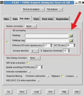
4.3.1. Field map-based EPI distortion correction ... 33

4.3.2. Functional data ... 35

4.3.3. Segmentation of structural data ... 37

4.4. Data analysis ... 37

4.4.1. Variability and Localisation of motor activation ... 37

4.4.2. CBF quantification methods ... 39

4.4.3. CBF quantification in Rest and Activation conditions... 40

4.4.4. SNR of perfusion-weighted images ... 41

4.4.5. CBF quantification: effect of anterior and posterior circulation ... 42

4.4.6. CBF quantification in GM and WM ... 42

Chapter 5 – Results and Discussion ... 43

5.1. EPI distortion correction ... 43

5.2. Comparing three functional protocols ... 46

5.3. Variability of extent and localisation of motor activation ... 51

5.4. CBF quantification: comparing the three methods ... 57

5.4.1. Inter-slices effect ... 59

5.5. CBF quantification in Rest and Activation conditions ... 62

5.5.1. Comparing ASL protocols ... 62

5.5.2. SNR of perfusion-weighted images ... 66

5.6. CBF quantification: effect of anterior and posterior circulation ... 68

5.7. CBF quantification in GM and WM ... 70

5.7.1. Partial volume effect correction ... 71

Chapter 6 - Conclusions... 75

6.1. Discussion ... 75

6.2. Future prospects ... 76

Bibliography ... 77

Appendix A - Appendix ... 81

A.1. BOLD-ASL fusion in Neuro3D... 81

A.2. Quantification maps Shell Script routine ... 84

A.3. Functional images for all subjects ... 88

A.4. Distance to the hand motor cortex ... 95

L

L

i

i

s

s

t

t

o

o

f

f

F

F

i

i

g

g

u

u

r

r

e

e

s

s

Figure 2.1: Relationship between an ideal map of brain activity and a metabolic and vascular map

that generate functional images ... 5

Figure 2.2: Brain anatomic structure ... 6

Figure 2.3: Representation of the principal areas of the motor cortex ... 7

Figure 2.4: Representation of a dissected brain showing the precentral knob ... 8

Figure 2.5: Schematic diagram of the main steps of cerebral energetic metabolism ... 9

Figure 2.6: Vascular system of the brain ... 9

Figure 2.7: The meaning of perfusion ... 10

Figure 2.8: Physiological changes that accompanying brain activation ... 14

Figure 3.1: Different image contrasts ... 16

Figure 3.2: (a) EPI sequence diagram and (b) EPI k-space coverage order during one TR ... 17

Figure 3.3: Schematic illustration of hemodynamic changes during neuronal activity ... 18

Figure 3.4: The typical hemodynamic response function (HRF) ... 19

Figure 3.5: Schematic description of a perfusion weighted image (_∆𝑀) obtained by subtraction of the labelled images from the control images, using the FAIR scheme ... 19

Figure 3.6: Continuous arterial spin labelling experiment ... 20

Figure 3.7: Pulsed arterial spin labelling experiment ... 21

Figure 3.8: A schematic of the idealized magnetisation difference curve with time ... 22

Figure 3.9: Vascular architecture showing the different vessel types that could pass through a typical tissue volume. ... 25

Figure 3.10: A comparison of inversion profiles a hyperbolic secant (HS) pulse, a frequency offset corrected inversion (FOCI) pulse, and the rectangular ideal pulse ... 25

Figure 4.1: Motor task performed by all volunteers ... 30

Figure 4.2: Illustration of a typical prescription of the imaging slab positions for a) BOLD and b) ASL experiments, from sagittal scout scan ... 30

Figure 4.3: Pulse sequence used for Q2TIPS ASL imaging ... 31

Figure 4.4: Layout of GUI interface for FUGUE (part of FEAT), for applying EPI distortion correction. 34 Figure 4.5: Design matrixes for the three functional protocols performed with FEAT ... 36

Figure 4.6: Localisation of the hand primary motor cortex ... 38

Figure 5.1: Field map image given by Neuro 3D from subject 4 ... 43

Figure 5.2: Phase difference image given by the scanner from subject 4... 44

Figure 5.3: Field map obtained with FSL ... 44

Figure 5.4: 3D representation of one slice of the unwrapped field map ... 45

Figure 5.5: Distorted and undistorted EPI images of functional data ... 45

Figure 5.6: BOLD statistical map obtained with FSL from Subject 2 ... 46

Figure 5.7: Perfusion maps obtained with Neuro 3D, for 16 axial slices in one subject ... 47

Figure 5.8: Fusion between BOLD t statistical map and the ASL difference map between 𝑟𝑒𝑙𝐶𝐵𝐹𝑎𝑐𝑡𝑖𝑣𝑎𝑡𝑖𝑜𝑛 and _{𝑟𝑒𝑙𝐶𝐵𝐹𝑟𝑒𝑠𝑡} maps ... 48

Figure 5.9: Activation Z maps superimposed on an example EPI image obtained for each experiment of each protocol from subject 2. ... 49

Figure 5.10: Activation Z maps (scale indicated in colorbar) obtained for each experiment of each protocol superimposed on the structural anatomic image from subject 2 ... 50

Figure 5.11: Orthogonal views (coronal, sagittal and axial) of inter-subject activation maps for BOLD (red), BOLDASL (green) and CBF (blue) in the MNI standard brain ... 53

Figure 5.12: 3D views of inter-subject activation clusters for BOLD (red), BOLDASL (green) and CBF (blue) ... 53

Figure 5.13: Localisation of the hand primary motor cortex... 54

Figure 5.14: A plot of the group mean Euclidean distance (in mm) from HMC points to CBF, BOLDASL and BOLD activation COGs ... 55

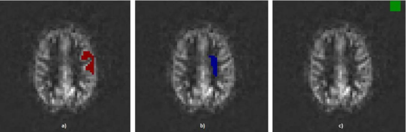
Figure 5.15: Representation of BOLD and CBF activations in coronal slices of subject 12 (presented from anterior to posterior, from left to right and from top to bottom in the figure), showing apparent activation over draining veins for BOLD experiment, but not for ASL. ... 56

Figure 5.16: A typical perfusion-weighted image from a 25 years old female subject ... 57

Figure 5.17: A plot of perfusion values (in ml/100g/min) computed using the 3 methods for each subject and group mean ... 58

Figure 5.18: Illustration of the positions of the 9 axial slices acquired ... 59

Figure 5.19: A plot of perfusion values (in ml/100g/min) across the 15 subjects calculated with the 3 methods for the firsts 7 slices ... 60

Figure 5.20: Relation between arterial blood transit time in arbitrary units (a. u.) and the distance travelled in z-axis (in a. u.) ... 61

Figure 5.21: Theoretical curves of PASL signal versus time calculated from Equation 3.3 ... 61

Figure 5.22: A plot of perfusion change (%) between the conditions of rest and activation ... 63

Figure 5.23: Quantitative perfusion maps (8 axial slices) provided by ASL protocols from subject 9 .. 65

Figure 5.24: A plot of the group mean SNR of grey matter (GM) and white matter (WM) calculated for both protocols ... 66

Figure 5.25: A schematic diagram for the assessment of the perfusion maps of each functional protocol ... 67

Figure 5.26: Position of ROI 1 and ROI 2 ... 68

Figure 5.28: Representation of the grey matter (GM) and white matter (WM), automatically

segmented, binary masks ... 70

Figure 5.29: A plot of CBF values (ml/100g/min) in automatically segmented grey and white matter masks for each subject. ... 70

Figure 5.30: Representation of the grey matter (GM) and white matter (WM) partial volume maps . 72 Figure 5.31: A plot of CBF values (in ml/100g/min) of grey and white matters for each subject with and without partial volume effects correction ... 72

Figure 5.32: A plot of the mean ratios of grey to white matter perfusion in each of 7 slices calculated with (right) and without (left) partial volume effects correction ... 73

Figure A.1: Functional images from Subject 1... 88

Figure A.2: Functional images from Subject 3... 88

Figure A.3: Functional images from Subject 4... 89

Figure A.4: Functional images from Subject 5... 89

Figure A.5: Functional images from Subject 6... 90

Figure A.6: Functional images from Subject 7... 90

Figure A.7: Functional images from Subject 8... 91

Figure A.8: Functional images from Subject 9... 91

Figure A.9: Functional images from Subject 10. ... 92

Figure A.10: Functional images from Subject 11. ... 92

Figure A.11: Functional images from Subject 12. ... 93

Figure A.12: Functional images from Subject 13. ... 93

Figure A.13: Functional images from Subject 14. ... 94

L

L

i

i

s

s

t

t

o

o

f

f

T

T

a

a

b

b

l

l

e

e

s

s

Table 3.1 - _𝑇1 and 𝑇2 values of CSF, grey and white matters for a magnetic field of 3 Tesla. ... 16

Table 4.1 – Functional data acquisition parameters ... 32 Table 4.2 - Perfusion quantification parameters used to calculate CBF ... 39

Table 5.1 - Results for the analysis of the location of activation measured by the centre of gravity (COG) and number of activated voxels for BOLD, BOLDASL and CBF ... 52

Table 5.2 – Results for the calculation of variance of MNI COGs for CBF, BOLDASL and BOLD activations

across _𝑁= 15 subjects ... 52 Table 5.3 – Group mean Euclidean distance between modalities (BOLD, BOLDASL and CBF) ... 56

Table 5.4 – CBF values in _𝑚𝑙/100𝑔/𝑚𝑖𝑛 in the GM mask for each subject calculated using the three methods ... 58 Table 5.5 – CBF values provided by each protocol for both conditions of rest and activation for the 15 subjects ... 63 Table 5.6 – Mean CBF values in _𝑚𝑙/100𝑔/𝑚𝑖𝑛 in GM and WM with and without partial volume effects (PVE) correction ... 73

Table A.1 – Group mean Euclidean distance (in mm) from HMC points (M3, M2, M1, CM and CC) to CBF, BOLDASL and BOLD activation COGs for all subjects ... 95

C

C

h

h

a

a

p

p

t

t

e

e

r

r

1

1

I

I

n

n

t

t

r

r

o

o

d

d

u

u

c

c

t

t

i

i

o

o

n

n

In research one scientist’s artefact is another scientist’s science.

Richard B. Buxton

1.1.

Objective of the thesis

Cognitive neuroscience has obtained a powerful tool to study human brain function with the advent of functional magnetic resonance imaging (fMRI). Most notably, imaging sequences based on the blood oxygen level dependent (BOLD) contrast are currently the predominant method used for activation studies. However, the complex nature of the BOLD signal complicates the interpretation of its changes [1]. Perfusion fMRI, based on arterial spin labelling (ASL) methods, offers a useful alternative to BOLD fMRI. The ASL methods can provide quantitative measures of perfusion, or regional cerebral blood flow (CBF), without the need for contrast agents. Because it is widely accepted that CBF is a physiological correlate of brain activity, ASL methods can be used to measure not only baseline perfusion but also its functional changes. Importantly, changes in CBF are believed to be more directly linked to neuronal activity than the BOLD signal, so that perfusion fMRI also has the potential to offer more accurate measures of the spatial location and magnitude of neural function [1, 2].

The work presented in this thesis is the first study of the recently commercially available ASL sequence from Siemens at the 3 Tesla scanner of Hospital da Luz Imaging Department. It contains not only a series of approaches for functional validation of this technique in healthy volunteers, by comparison with BOLD contrast, but it also accomplishes some important quantification issues. The main objective was to provide the first results and comparative analyses between these two alternative and complementary fMRI techniques for clinical applications.

This thesis comprises the analysis and optimisation of the ASL sequence for functional studies, as well as the evaluation of its potential to provide quantitative values of CBF. Also, it presents some of the benefits and possible limitations of this technique by giving a small summary of its physical principles and assumptions.

1.2.

Previous work

tissue can now be performed using fMRI techniques. Although the BOLD effect is most often used in brain activation studies, a drawback of this technique is that it only provides indirect information on the change in activity between one state and another, and does not provide a quantitative measure of cerebral activity. It provides no information, for example, on the resting or chronic perfusion state [1]. Moreover, when longitudinal experimental designs are employed in order to investigate processes taking place over long periods of time, BOLD information may not be valid.

There are two classes of MRI techniques that do provide measures of the resting perfusion state [2]. The first class is based on the use of an extrinsic tracer, namely intravascular contrast agents that alter the magnetic susceptibility of blood. The second is ASL, which uses magnetic labelling of inflowing arterial blood as a free-diffusible tracer, to obtain perfusion images. This technique is potentially quantitative and allows the extraction of absolute values for CBF. The main advantages of ASL over the first class technique, and over the majority of perfusion techniques, are improved spatial resolution and complete non-invasiveness requiring no potentially harmful contrasts injection. For that reason, it can be repeated without limit, and can be used to study normal physiology and its variations with time. It also has the potential to provide quantitative functional activation maps, which cannot be accomplished with BOLD fMRI studies [1].

The main ASL drawbacks are related to its intrinsically low signal-to-noise ratio (SNR) and the short life time of the label. The introduction of higher field scanners (like the 3 Tesla scanner) greatly benefited this technique, by improving the SNR of perfusion-weighted maps. Furthermore, in the last decade a number of improvements of the labelling strategies were introduced, which aimed to solve some of the problematic technical issues such as magnetisation transfer effects, and others [3].

Both BOLD and ASL methods are able to provide functional information of the brain, but they are quite different, and measure different aspects of brain hemodynamics. Previously, a number of fMRI studies made comparisons between ASL and BOLD contrast. Most of these studies were performed using BOLD acquired simultaneously with the ASL technique. Some of them suggest that perfusion changes have greater spatial resolution than BOLD changes during functional activation. Indeed, standard BOLD fMRI studies show apparent activation over relatively distant draining veins, which is not observed using perfusion contrast, suggesting that ASL may more accurately localise the region of neuronal activity [4]. Moreover, between-subject variability has been found to be smaller when measured with perfusion fMRI as compared with BOLD fMRI [5, 6], which implies that blood flow changes may be more consistent across subjects than changes in BOLD contrast. Another interesting result is that, as long as the same procedure and parameters are consistently used, more reproducible results have been achieved with ASL than BOLD [6] (see the review paper [7] for further comparisons between these two techniques).

1.3.

Structure of the thesis

This thesis begins by providing some background theory in Chapter 2, describing the basic biological and physiological aspects of brain function. Also, some of the most important neuroimaging techniques are mentioned, with particular emphasis on those that measure perfusion changes.

In Chapter 3, functional MRI techniques are introduced, including the theoretical background and main implementations of ASL. In particular, the perfusion quantification methods, and some of the problems and pitfalls involved, are thoroughly discussed.

The materials and methods used for this study are described in Chapter 4. It includes the methodology applied for the acquisition and processing of the images, as well as for the analyses and evaluation of the results. The subsequent approaches developed for the statistical analysis are also explained in this chapter.

C

C

h

h

a

a

p

p

t

t

e

e

r

r

2

2

F

F

u

u

n

n

c

c

t

t

i

i

o

o

n

n

a

a

l

l

N

N

e

e

u

u

r

r

o

o

i

i

m

m

a

a

g

g

i

i

n

n

g

g

The purpose of understanding the functional organisation of the human brain has inspired many neuroscientists for well over 100 years [1], but the experimental tools to measure and map brain activity have been slow to develop.

Neuronal activity is too difficult to localise without placing electrodes directly in the brain [1, 2]. Electric and magnetic fields measured at the scalp provide information on electric events within the brain, which allow the estimation of the location of a few sources of activity. However, precise localisation of the metabolic activity that follows neural activity is much more feasible and allows to produce a detailed map of the pattern of activation [1]. This is the basis of most of the functional neuroimaging techniques used today, including positron emission tomography (PET) and functional magnetic resonance imaging (fMRI). In fact, the physiological basis of these methods is the fact that brain cell activity is associated with local changes in metabolism [2], namely with glucose and oxygen consumption, and consequently also with haemodynamics, namely blood oxygenation, cerebral blood flow (CBF) and cerebral blood volume (CBV). Somehow nature performs a functional convolution of brain cell activity, _𝑓(𝑥,𝑡), at a given location _𝑥 and time _𝑡 with the function “_𝑔” which

produces a certain change in metabolism and in haemodynamics [2]. The result is a map of metabolic and vascular events,_𝑔(𝑓(𝑥,𝑡)), associated with changes in brain activity (see Figure 2.1).

So, in order to understand the functional images obtained with these methods, it is important to understand the relationship between local brain activity and the physiological parameters which are measured, and also the relationship between these physiological parameters and the obtained functional image (Figure 2.1). In this chapter these issues are discussed.

Figure 2.1: Relationship between an ideal map of brain activity and a metabolic and vascular map that generate functional images (adapted from [1]).

2.1.

Brain structure

The normal adult human brain typically weighs between 1 and 1.5 kg and has an average volume of 1600 cm3 _{[9], but receives 25% of all body blood flow. The basic anatomical brain structure can be}

seen in Figure 2.2 (a).

Figure 2.2: Brain anatomic structure. (a) Representation of temporal, parietal, frontal and occipital lobes. (b) Some of the different types of tissues in the brain.

This organ is composed of three main parts: the forebrain, midbrain and hindbrain [9]. The cerebellum, that is visible at the back of the brain (Figure 2.2 (a)), together with the pons and the medulla, compose the hindbrain. The medulla, pons and midbrain are often referred collectively as the brain stem. These structures are almost completely enveloped by the cerebellum and telencephalon, with only the medulla visible as it merges with the spinal cord [9]. As for the forebrain, it is composed by the cerebrum, thalamus and hypothalamus. The cerebrum is the largest

part of the human brain and is divided into sections called “lobes” (Figure 2.2 (a)): the frontal, parietal, occipital and temporal and insular lobes [9].

In the next subsection, a more thorough review of the cerebrum is shown, as this work is mainly focused in tissue detection in this particular area of the brain.

2.1.1.

Cerebral cortex

The cerebrum is composed of an outer layer of grey matter, internally supported by deep brain

white matter. It is responsible for the so called “higher functions”, such as thinking and cognition [8]. Grey matter consists of cell bodies of neurons, while white matter consists of axons that connect neurons. These are often surrounded by a fatty insulating cover called myelin, which gives the white matter its distinctive colouration (see Figure 2.2 (b)). The function of this fatty sheath is to insulate nerve endings, enable smoothly movements of brain signals and to accelerate the transmission of the nerve signals [9].

The brain is surrounded by the meninges and the subarachnoid space, which separates the soft brain tissues and spinal cord from the hard surrounding bones like skull and vertebrae. This space and the cavities located inside the brain, the ventricular system, are filled with cerebrospinal fluid (CSF), which is believed to be produced by the choroid plexus [9] (Figure 2.2 (b)). The CSF is very similar to blood plasma and is the other supplier of nutrients to the brain.

2.2.

Brain functional anatomy: the hand motor cortex

The cortical anatomy of cerebral gyri is complex and presents tremendous intra- and inter-subject variability [9]. Therefore, the identification of specific cortical regions based only on morphologic features can be challenging. The presence of space-occupying lesions in the brain, such as tumors or vascular malformations, can further complicate this procedure by distorting normal anatomy, thereby making the identification of specific cortical regions difficult or impossible.

Previous studies have demonstrated that the motor function is controlled by four major regions in the frontal lobe: the primary motor cortex (M1), which lies just anterior to the central sulcus on the precentral gyrus, the supplementary motor area (SMA), the premotor area and the cingulate motor area which lie just anterior to M1 (shown in Figure 2.3). The motor cortex located on the left side of the brain controls movement on the right side of the body [9].

Figure 2.3: Representation of the principal areas of the motor cortex (adapted from [9]).

The cortical representation of motor hand function, which allowed the development of the

concept of “homunculus”, is known to be located in the superior aspect of the precentral gyrus [10]. Even though functional techniques have recently permitted the identification of anatomic regions based on the correspondence with regions of activation, the knowledge of pure anatomic landmarks of the cerebral cortex remains of fundamental importance in research and everyday clinical practice. Yousry et al. [10] described the hand motor cortex (HMC) in dissected brains or computed tomography and MR imaging as having the shape of a typical hook on the sagittal plane and a structure like an inverted omega (_Ω) or epsilon (ε) on the axial plane (see Figure 2.4). They also localized blood oxygen level dependent (BOLD) activation, obtained during hand movement exactly on the omega region of the precentral gyrus.

Figure 2.4: Representation of a dissected brain showing the precentral knob (indicated by arrows), which can look like an inverted omega (A) or a horizontal epsilon (B) when cut axially, and like a hook when cut sagittaly (C) [10].

2.3.

Energy metabolism in the brain

Like in all organs, energy metabolism in the brain is necessary for the basic processes of cellular work, such as chemical synthesis and chemical transport [1]. Still, the particular work done by the brain, which is the generation of electrical activity required for neuronal signalling, such as the generation of an action potential and the release of neurotransmitter at a synapse, requires a high level of energy metabolism [11].

In biologic systems the free energy necessary for these tasks is primarily stored in relative proportions of three nucleotides: adenosine triphosphate (ATP), adenosine diphosphate (ADP) and adenosine monophosphate (AMP), being ATP the main source of energy for cells [11]. ATP production is dependent on the combination of glucose and oxygen. The metabolism occurs in two stages: glycolysis and the trans-carboxylic acid (TCA) cycle (also known as the citric acid cycle or the Krebs cycle) [11, 12]. Glycolysis does not require oxygen but the further metabolism of glucose though the TCA cycle requires oxygen and produces much more ATP (see Figure 2.5).

Oxidative glucose metabolism involves many steps and different reactions which are catalyzed by different enzymes within the cell. At the end of the process, carbon dioxide and water are produced, and an additional 38 ATP molecules are created. The overall metabolism of glucose is then

𝐶6𝐻12𝑂6+ 6𝑂2→6𝐶𝑂2+ 6𝐻2𝑂 (+38𝐴𝑇𝑃)

Figure 2.5: Schematic diagram of the main steps of cerebral energetic metabolism (adapted from [1]).

2.4.

Cerebral blood flow

The vascular system that supplies blood to the brain is organised on a spatial scale that spans a range of four orders of magnitude, from the diameter of a capillary (about 10 _𝜇𝑚) to the size of a major artery (about 3 _𝑐𝑚) [1]. The complexity of the vascular system of the brain can be appreciated from images in Figure 2.6. In short, the architecture of the vascular tree shows distinct organisation on a spatial scale as small as a few hundred micrometers.

Figure 2.6: Vascular system of the brain [1]. In the left image there’s an MR angiogram showing the main arteries supplying blood to brain tissues, and the veins which drain that tissues. In the right image a microscopic view is presented, showing the complex geometry of small vessels: arterioles, capillaries and venules.

2.4.1.

The Meaning of Perfusion

The term perfusion is generally used to describe the process of nutritive delivery of arterial blood to a capillary bed in the tissue and cells. Since cerebral haemodynamics is one of the key aspects in functional neuroimaging, it is important to describe it in terms of a number of clearly defined variables. One of these variables is the cerebral blood flow, defined as the rate of delivery of arterial blood to the capillary beds of a particular mass of tissue [1], as illustrated in Figure 2.7 (a). In this idealized tissue vasculature, the flow rates through both capillary beds are designated _𝐹1 and 𝐹2 (expressed in millilitres per minute), and if these vessels feed a volume of tissue 𝑉, then CBF is simply (𝐹₁+𝐹₂)/𝑉. For convenience, a common unit for CBF is millilitres of blood per 100 grams of tissue per minute, and a typical average value in the human brain is 60 𝑚𝑙/100𝑔/𝑚𝑖𝑛 [1]. However, in some circumstances it is convenient to express CBF as flow delivered to a unit volume of tissue rather than a unit of mass of tissue. For instance, in imaging applications a signal is measured from a particular volume in the brain, and the actual mass of tissue within that volume is not known. Because the density of brain is close to 1 𝑔/𝑚𝑙 [1], CBF values expressed in these units are similar (it means that 60 𝑚𝑙/100𝑔/𝑚𝑖𝑛 is equivalent to 0.01 𝑠−1).

The cerebral blood volume (CBV) is the fraction of the tissue volume occupied by blood vessels, and a typical value for the brain CBV is 4% (CBV = 0.04) [1]. The CBV is a dimensionless number (millilitres of blood vessel per millilitre of tissue), and generally refers to the entire vascular volume

within the tissue. However, in some occasions it’s important to subdivide total CBV into arterial,

capillary and venous volumes, where typical estimate numbers are 5% for the arterial volume and 95% equally divided for capillaries and veins [1].

The velocity of blood in the vessels is also an important physiological parameter, which varies from tens of centimetres per second in large arteries to as slow as one millimetre per second in the capillaries [1].

Figure 2.7: The meaning of perfusion (adapted from [1]). (a) Illustration of blood vessels within a small element tissue for cerebral blood flow definition. (b) Demonstration of the incapacity to calculate CBF with blood volume and velocity.

CBF does not explicitly depend on either blood volume or the velocity of blood in the vessels, i.e., an increase in CBF with brain activation could occur through a number of different changes in blood volume or blood velocity. In Figure 2.7 (b) two idealized capillary beds are shown, one with two sets of shorter capillaries, and one with a single set of capillaries twice as long. Both beds show the same blood velocity and CBV. However, CBF is twice as large in the top bed with two sets of shorter capillaries. The missing piece that does differ between the two scenarios and is responsible for this difference is the capillary transit time [13]. In the bottom bed the capillary transit time is twice as long. And it is transit time, rather than blood velocity, that is directly connected to CBV and CBF. The relation between CBV, CBF and the mean transit time (_𝑀𝑇𝑇) through the volume CBV is known as the central volume principle, and is defined as:

𝑀𝑇𝑇=𝐶𝐵𝑉/𝐶𝐵𝐹

For a CBF of 60 𝑚𝑙/100𝑔/𝑚𝑖𝑛 (0.01 𝑠−1) and a typical CBV of 4%, from this equation _𝑀𝑇𝑇 is 4 𝑠. In summary, the definition of CBF involves some subtleties that have to be considered when we want to measure it. Some of these subtleties consist in particular properties of the measuring technique that we use. For this reason an accurate approach is necessary to properly measure CBF.

2.4.2.

Measuring CBF

Numerous imaging techniques have been developed and applied to evaluate brain hemodynamics [14]. Most of those techniques rely on mathematical models developed at the beginning of the century, giving similar information about brain hemodynamics in the form of different parameters such as CBF or CBV. For that purpose, they use different tracers to mimic perfusion and have different physical principles and different technical requirements.

2.4.2.1.

Diffusible vs. Intravascular tracers

The various tracers used in brain studies usually fall into one of two basic classes, diffusible tracers and intravascular tracers, which differ in their volume of distribution [1, 2]. Nitrous oxide, for example, freely diffuses out the capillary bed and fills the entire tissue space, so its volume of distribution is essentially the whole brain volume. On the other hand, an agent that remains in the blood has a volume of distribution that is much smaller, only about 4% of the total brain volume [1]. For an intravascular agent the time constant for the venous blood to equilibrate with the arterial blood is corresponding shorter, or in other words, for the same flow, the volume of distribution of an intravascular agent is quickly filled because the blood volume is only a small fraction of the total tissue volume [1].

blood) is measured over time, once the agent has reached equilibrium within its volume of distribution, the tissue concentration of the agent is independent of flow but provides a robust measure of the volume of distribution. Therefore, an intravascular agent provides a robust measurement of CBV, because that is its volume of distribution, but a poor measurement of flow, because it equilibrates too quickly. In contrast, a diffusible tracer provides a robust measurement of flow because the time for equilibrium is much longer.

These basic ideas suggest that the perfusion techniques applied to measure local CBF use diffusible tracers.

2.4.2.2.

Techniques to measure CBF

The main imaging techniques dedicated to brain hemodynamics are positron emission tomography (PET), single photon emission computed tomography (SPECT), Xenon-enhanced computed tomography (XeCT), dynamic perfusion computed tomography (PCT), Doppler ultrasound, MRI dynamic susceptibility contrast (DSC) and arterial spin labelling (ASL).

PET is a powerful diagnostic tool, considered in early times the gold standard technique for brain perfusion evaluation [14], that provides tomographic images of quantitative parameters describing regional CBF (rCBF), regional CBV (rCBV), regional oxygen extraction fraction (rOEF), regional cerebral metabolic rate of oxygen (rCMRO2) or glucose, neurotransmission processes, etc. These images result

from the use of different substances of biological interest labelled with positron emitting radioisotopes. The most commonly used tracer to measure CBF is H215O [15], which is administered

directly by intravenous injection. A few minutes scan is performed and its results combined with an arterial blood sampling measurement, performed in order to obtain the input function, leads to quantitative CBF maps.

SPECT was introduced soon after PET. Besides some technical aspects, like the equipment involved, the main difference between SPECT and PET is that the first one uses radioisotopes which emit gamma photons, such as 99mTc [15]. Perfusion PET and SPECT methods afford whole brain coverage and provide valuable information, giving quantitative CBF maps [14, 15]. However, the spatial resolution of these nuclear imaging studies ranges from _≈4 to 6 𝑚𝑚 [14]. Its clinical applications are still limited due to their high price and specific technical requirements. In addition to the access to radiopharmaceuticals, PET requires the access to a cyclotron near the administration local. Furthermore, in PET or SPECT examinations, the whole body is exposed to radiation.

advantage is its rapid elimination, which makes repeated scanning under different conditions possible. Nonetheless, Xe is a narcotic gas, and even if it was used in low doses, some side effects can be seen, like euphoria, raising the need of permanent medical assistance during the imaging procedure. Moreover, dynamic PCT and XeCT use ionizing radiation, and as PET and SPTEC methods, they are not completely non-invasive techniques [15].

Although different in nature from other imaging techniques described hereby and accordingly limited in spatial resolution, Doppler ultrasound offers the advantage of being non-invasive and repeatable as often as clinically indicated at the patient’s bedside [14]. It doesn’t involve radiation, doesn’t require any contrast medium, and is free of any known adverse effect. Considering these facts, ultrasound Doppler technology may represent a convenient tool for the measurement of blood flow volume in the internal carotid artery as a correlate for CBF in the corresponding hemisphere [14].

MRI also provides two approaches to measuring CBF. Like first-pass PCT, the first of these approaches, DSC, implies the administration of a contrast agent [14, 15] that remains intravascular. In addition, MR contrast agents alter image intensity indirectly affecting the surrounding tissues. The other MRI method for imaging CBF, ASL, does not require administration of a contrast agent, and provides direct measures of CBF changes [15]. Most importantly, this MR method requires neither exposure to form of radiation (as XeCT), nor administration of a contrast agent (as MR DSC), and measures can be repeated as often as required. A more detailed discussion of this last technique will be given in Chapter 3.

2.5.

Brain Activation

The real nature of the coupling between CBF and CMRO2 during activation is still debated.

However, the tomographic techniques have provided experimental data for the generation of some theories that explain the energetic metabolism of the brain.

The primary finding is that CBF increases substantially during brain activation [16]. The increase is localised and is a graded response in the sense that the magnitude of the flow change is often correlated with other measures of the degree of neural activity. The second finding is that CMRO2

increases much less than CBF [16]. The main reason for that or at least the most accepted one nowadays, is that this unclear disconnection between CBF and CMRO2 is due to a large and

disproportional essential increase on CBF to supply a small increase of the oxygen consumption during activation [17]. This oxygen limitation model is based on two assumptions: the first one is that the supply of oxygen to the tissue is limited by BBB, which means that only a small rate of the supplied oxygen is available for metabolism. The second one is that CBF increasing is accompanied by an increase of blood velocity in the capillaries rather than the capillary recruitment [17]. In summary, the result of this imbalance in the changes of CBF and CMRO2 is a substantial drop in oxygen

extraction like is shown in Figure 2.8.

conditions [17]. With the introduction of techniques such as fMRI, it was possible to piece together an empirical picture of the physiological changes that accompany brain activation and form the basis for functional neuroimaging.

C

C

h

h

a

a

p

p

t

t

e

e

r

r

3

3

F

F

u

u

n

n

c

c

t

t

i

i

o

o

n

n

a

a

l

l

M

M

a

a

g

g

n

n

e

e

t

t

i

i

c

c

R

R

e

e

s

s

o

o

n

n

a

a

n

n

c

c

e

e

I

I

m

m

a

a

g

g

i

i

n

n

g

g

Functional magnetic resonance imaging (fMRI) provides a sensitive, non-invasive tool for mapping patterns of activation in the working human brain. However, how this tool works is far from obvious, and to understand the strengths and limitations of fMRI it is necessary to delve into the nature of the magnetic resonance (MR) signal and how it can be measured and affected by brain activation.

3.1.

Physics principles of MRI

Magnetic Resonance Imaging (MRI) is a non-invasive imaging technique that allows to produce high quality images of living organisms [1]. This technique is also known as magnetic resonance tomography or nuclear magnetic resonance.

MRI is based on the principles of nuclear magnetic resonance. It measures spatial variations in the phase and frequency of the radio-frequency energy being absorbed and emitted by the imaged object [18].

There is a huge amount of atoms in the human body. The ones with nuclei with an odd number of protons and neutrons possess a property called spin, which is its intrinsic angular momentum and can attain any value multiple of 1/2. When these spins are placed in a strong external magnetic field (_𝐵0) they precess around an axis along the direction of the field, aligning in two energy “eigenstates”

(analogous to the Zeeman Effect): one low-energy and one high-energy, which are separated by a very small splitting energy [18]. This precession frequency_𝜈 is called the Larmor frequency and is obtained (with the gyromagnetic ratio of nucleus, 𝛾) from the Larmor equation:

𝛾𝐵0 =𝜈 Equation 3.1

After exposing the object of study to a magnetic field, a transient radio frequency (RF) pulse at the characteristic Larmor frequency is briefly applied, in a plane perpendicular to 𝐵₀. This RF pulse excites some of the spins in the lower energy state at their resonant frequency, disturbing the aligned hydrogen nuclei, thus causing a disruption of the equilibrium. From this disturbance of equilibrium, two effects arise: longitudinal and transverse magnetisation [18]. So, the RF pulse causes an oscillatory effect on the component of the magnetisation vector (_𝑀) parallel to the z axis, and a small component of the magnetisation will be in the x-y axis, which can be detected. The angle that the net magnetisation vector rotates is commonly called the flip angle [19].

decay (FID) [19]. In an idealized MR experiment, the FID decays approximately with a time constant called_𝑇2, which is the time that takes transverse magnetisation to decrease 63% of its value when the RF pulse is turned off. However, in practical MRI small differences in the static magnetic field at different spatial locations (inhomogeneities) cause the Larmor frequency to vary across the body creating destructive interference which shortens the FID. The time constant for the observed decay of the FD is called the _𝑇2∗ relaxation time, and is always shorter than_𝑇2. Also, when the RF pulse is turned off, the longitudinal magnetisation starts to recover exponentially with a time constant_𝑇1, which is the time for the magnetisation to return to 63% of its original length [19].

In MRI, the static magnetic field is caused to vary across the body (by applying field gradients using appropriate coils), so that different spatial locations become associated to different precession frequencies. Usually these field gradients are pulsed, and it is the almost infinite variety of RF and gradient pulse sequences that gives MRI its versatility. The application of a field gradient destroys the FID signal, but this can be recovered and measured by a refocusing gradient (to create a so-called

gradient echo), or by a RF pulse (to create a so-called spin echo). The whole process can be repeated when some longitudinal relaxation has occurred and the thermal equilibrium of the spins has been more or less restored [19].

Typically in soft tissues _𝑇1is around one second while_𝑇2 and _𝑇2∗ are a few tens of milliseconds, but these values vary widely between different tissues (and different _𝐵0), giving MRI its tremendous soft tissue contrast (see Table 3.1) [19].

Table 3.1

𝑇1 and 𝑇2 values of CSF, grey and white matters for a magnetic field of 3 Tesla [20]

Tissue _𝑻𝟏 (𝒎𝒔) 𝑻_𝟐 (𝒎𝒔)

White matter 832 110

Grey matter 1331 80

CSF 2500 250

Thus, image contrast is created by differences in the strength of the MR signal recovered from different locations within the sample, which depends upon the relative density of excited nuclei (usually water protons), on differences in relaxation times of those nuclei after the pulse sequence [18]. Furthermore, image contrast relies on other parameters (controlled by users): the echo time (TE) which is the time between the centre of the initial RF pulse (in a pulse sequence) and the centre of the signal echo formed by that pulse, and the repetition time (TR) which is the amount time that exists between successive excitation pulse sequences (see Figure 3.1) [19].

3.2.

Image acquisition

The quality and contrast of the image acquired with MRI can be manipulated by the use of different image acquisition techniques. The main steps usually consist on slice selective excitations, frequency encoding and phase encoding, which result in data being collected in a spatial frequency space – the k-space1_{. Image reconstruction is then accomplished by performing a 2D inverse Fourier}

transform of the raw data. The exact timings and characteristics of the acquisition determine the resolution and contrast of the image [19]. Many methods of image acquisition have been developed in order to reduce the image acquisition time, which is very useful for functional studies.

Gradient-echo (GE) - echo-planar imaging (EPI) sequences are the commonly used in such applications. This acquisition module is based on the collection of the data necessary to reconstruct an image using one set of echoes after a single RF excitation and a short phase encoding gradient between each echo [14]. The EPI sequence diagram is showed in Figure 3.2 (a).

Figure 3.2: (a) EPI sequence diagram and (b) EPI k-space coverage order during one TR (adapted from [14, 19]).

Figure 3.2 (b) shows the k-space sampling trajectory determined by the EPI sequence. All k-space lines are acquired in only one shot and each line is acquired in the opposite direction relatively to the previous one. This effect results in the phase accumulation (N) in different directions in odd and even lines of the k-space. After image reconstruction it leads to an N/2 shift of the object representation, which can lead to the Nyquist ghosting effect. The main advantages of EPI readout are the short acquisition time, efficiency, regular k-space coverage and acceptable signal to noise ratio (SNR), and it can be combined with many spin preparation methods. However, the EPI acquisition is very sensitive to susceptibility induced field changes and inhomogeneities which may be useful for fMRI studies [21]. However, this property can also lead to signal drop-out and image distortions. In fact, image distortion occurs frequently near the sinuses, due to the magnetic field differences between the air (in the sinuses) and the brain tissues [14]. The readout, x, direction of the k-space is acquired with a high bandwidth (fast acquisition), while the phase-encoding direction, y, is acquired more slowly. The image quality depends on the echo spacing for a given resolution and phase errors, and consequently geometric distortions, appear predominantly in the phase encoding direction.

1

3.3.

BOLD functional MRI

Although susceptibility effects can produce artefacts when imaging the brain (as mentioned in the previous section), they are the basis of the generation of the blood oxygen level dependent (BOLD) contrast that is the basis of most functional MRI studies [22].

The magnetic susceptibility effect at the basis of BOLD experiments arises from the biophysics of the haemoglobin molecule, which provides oxygen required for aerobic energy metabolism [23]. As blood leaves the lungs, oxygen becomes loosely and reversibly bonded to an iron atom that lies at the center of the heme molecule within the haemoglobin complex. When delivered to tissue, oxygen separates from the heme molecule exposing electrons from the iron atom. The unpaired iron electrons alter the lines of the magnetic field near the deoxyhemoglobin molecule, which causes slight dephasing of the spins of the hydrogen nuclei in proximal water molecules of both blood vessels and adjacent tissues [23, 24]. These effects occur because haemoglobin is diamagnetic when oxygenated but paramagnetic when deoxygenated. The MR signal of blood is therefore slightly different depending on the level of oxygenation. Higher BOLD signal intensities arise from increases in the concentration of oxygenated haemoglobin since the blood magnetic susceptibility now more closely matches the tissue magnetic susceptibility [23].

Chapter 2 laid the foundation for understanding how fMRI based on BOLD effect works. Brain activation is characterized by a drop in the local oxygen extraction fraction (OEF) and a corresponding drop in the local concentration of deoxyhemoglobin, which produces a small increase in the MR signal (see Figure 3.3) [24]. Thus, using deoxyhemoglobin as an endogenous tracer, regional brain activation can be mapped with _𝑇2∗ sensitive pulse sequences, such as the GE sequence.

Figure 3.3: Schematic illustration of hemodynamic changes during neuronal activity [25]. From the basal state (resting) to activated state a decrease of deoxyhemoglobin concentration occurs in the capillaries and venules, resulting in an increase in the BOLD signal intensity.

In summary, BOLD contrast does not reflect a single physiological process, but rather represents the combine effects of cerebral blood flow (CBF), cerebral blood volume (CBV) and cerebral metabolic rate of oxygen (CMRO2) [24]. Furthermore, the sluggish response of the vascular system to

drop followed by the rise to a single maximum, a decline, and an undershoot before returning to baseline [21]. The HRF characteristics vary between different regions of the brain and depend on the stimulus and its duration [26]. A detailed biophysical explanation of the complex shape of the BOLD signal is a current area of research.

Figure 3.4: The typical hemodynamic response function (HRF): BOLD response to a brief stimulus (adapted from [18]).

3.4.

Perfusion functional MRI

–

ASL

Arterial spin labeling (ASL), also called arterial spin tagging, is a non-invasive MRI method to measure brain perfusion.

The overall goal of all existing ASL techniques is to produce a flow-sensitized image or labelled image and a control image in which the static tissue signals are identical, but where the magnetisation of the inflowing blood differs [27]. The subtraction control-label (_{𝑀𝑐𝑜𝑛𝑡𝑟𝑜𝑙 − 𝑀𝑡𝑎𝑔}) yields a signal difference ∆𝑀 that directly reflects local perfusion, because the signal from stationary tissue is completely eliminated (Figure 3.5). The label is usually performed by inverting or saturating the spins of water molecules of the blood supplying the imaged region [27, 28]. Once the labelled blood spins are allowed to reach the capillary bed, which is accomplished with a delay between the labelling and image acquisition, they exchange with tissue water and thereby give rise to the perfusion signal. The signal difference, which is only 0.5−1.5% of the full signal, depends on many parameters such as the flow itself, the _𝑇1 of blood and tissue, as well as the time it takes blood to travel from the labelling slab to the imaging region [27]. Multiple repetitions are needed for ensuring sufficient SNR, and a model of the perfusion signal is usually used in order to quantify CBF.