Dissertation submitted in partial fulfillment of the requirements for the degree of Master of Science in Biomedical Engineering

Bachelor Degree in Biomedical Engineering Sciences

Assessment of a multi-measure functional

connectivity approach

Dissertation submitted in partial fulfillment of the requirements for the degree of

Master of Science in

Biomedical Engineering

Adviser: Alexandre Andrade, Assistant Professor,

Institute of Biophysics and Biomedical Engineering of the University of Lisbon

Co-adviser: Ricardo Vigário, Assistant Professor,

Faculty of Sciences and Technology of the Nova Univer-sity of Lisbon

Examination Committee

Chairperson: Carla Quintão Pereira Raporteur: Maria Margarida Silveira

Copyright © Miguel Claudino Leão Garrett Fernandes, Faculty of Sciences and Technol-ogy, NOVA University of Lisbon.

The Faculty of Sciences and Technology and the NOVA University of Lisbon have the right, perpetual and without geographical boundaries, to file and publish this disserta-tion through printed copies reproduced on paper or on digital form, or by any other means known or that may be invented, and to disseminate through scientific reposito-ries and admit its copying and distribution for non-commercial, educational or research purposes, as long as credit is given to the author and editor.

This document was created using the (pdf)LA_{TEX processor, based in the “novathesis” template[1], developed at the Dep. Informática of FCT-NOVA [2].}

I wish to thank to my adviser, professor Alexandre Andrade, and to PhD Susana Santos for all their guidance, availability and kindness throughout the whole process of writing this thesis. It was a pleasure working with both of you. To PhD Pedro Guimarães for his availability, to professor Fernando Batista of ISCTE also for his availability and especially for his interest and enthusiasm, to professor Branislav Gerazov for his brief but invaluable help in my introduction to machine learning. Also, to everyone I had the opportunity to meet at the institute and that made me feel welcomed there. Specially, to MSc. Diogo Duarte for always sharing his wise thoughts on all my questions and to his organization of many journal club meetings at the institute, to which I had the pleasure of attending.

Because this work really is the product of five years of education, I would like to thank professor Ricardo Vigário and to all my professors at the Faculty of Sciences and Technology of the Nova University of Lisbon and specially to those who cultivated my passion for science and for teaching with their enthusiasm, knowledge and patience. Also, for the same reasons, to the ones at the Polytechnic of Milan during my Erasmus program in Italy.

To my family for their support, for their belief in me and for allowing me to pursue my life goals, thank you. Shall we keep playing many more chess games, grandfather! (and shall you keep winning them too).

To all my friends for making this five-year journey a much better one and specially to Marta Pinto for her help in this thesis and for everything else, but mostly for her invaluable friendship. I hope you all keep making part of my life in some way or another for years to come.

it everyone you love, everyone you know, everyone you ever heard of, every human being who ever was, lived out their lives. The aggregate of our joy and suffering, thousands of confident religions, ideologies, and economic doctrines, every hunter and forager, every hero and coward, every creator and destroyer of civilization, every king and peasant, every young couple in love, every mother and father, hopeful child, inventor and explorer, every teacher of morals, every corrupt politician, every "superstar," every "supreme leader," every saint and sinner in the history of our species lived there - on a mote of dust suspended in a sunbeam.

Eff_{orts to find di}ff_{erences in brain activity patterns of subjects with neurological and}

psychiatric disorders that could help in their diagnosis and prognosis have been increas-ing in recent years and promise to revolutionise clinical practice and our understandincreas-ing of such illnesses in the future. Resting-state functional magnetic resonance imaging (rs-fMRI) data has been increasingly used to evaluate said activity and to characterize the connectivity between distinct brain regions, commonly organized in functional connectiv-ity (FC) matrices. Here, machine learning methods were used to assess the extent to which multiple FC matrices, each determined with a diff_{erent statistical method, could change}

classification performance relative to when only one matrix is used, as is common practice. Used statistical methods include correlation, coherence, mutual information, transfer en-tropy and non-linear correlation, as implemented in the MULAN toolbox. Classification was made using random forests and support vector machine (SVM) classifiers. Besides the previously mentioned objective, this study had three other goals: to individually in-vestigate which of these statistical methods yielded better classification performances, to confirm the importance of the blood-oxygen-level-dependent (BOLD) signal in the fre-quency range 0.009-0.08 Hz for FC based classifications as well as to assess the impact of feature selection in SVM classifiers. Publicly available rs-fMRI data from the Addiction Connectome Preprocessed Initiative (ACPI) and the ADHD-200 databases was used to per-form classification of controls vs subjects with Attention-Deficit/Hyperactivity Disorder (ADHD). Maximum accuracy and macro-averaged f-measure values of 0.744 and 0.677 were respectively achieved in the ACPI dataset and of 0.678 and 0.648 in the ADHD-200 dataset. Results show that combining matrices could significantly improve classification accuracy and macro-averaged f-measure if feature selection is made. Also, the results of this study suggest that mutual information methods might play an important role in FC based classifications, at least when classifying subjects with ADHD.

Keywords: fMRI, classification, functional connectivity matrices, SVM, feature selection,

A identificação de diferenças nos padrões de atividade cerebral de indivíduos com do-enças mentais poderá revolucionar o conhecimento relativamente às causas subjacentes, assim como a capacidade de diagnóstico e prognóstico em contexto clínico. A imagem por ressonância magnética funcional em repouso (rs-fMRI) tem sido largamente utilizada para avaliar esta atividade e caracterizar a conetividade entre diferentes regiões cerebrais. Esta informação é normalmente organizada em matrizes de conetividade funcional (FC). Neste estudo, utilizaram-se técnicas de aprendizagem automática para avaliar de que forma diferentes matrizes de conetividade, usadas em simultâneo, alterariam a qualidade de uma classificação automática relativamente ao caso comum em que apenas uma matriz é utilizada. Os métodos estatísticos calculados com o programa MULAN incluem: correla-ção, coerência, informação mútua, transferência de entropia e ainda correlação não linear. A classificação fez-se com recurso arandom forestse asupport vector machines(SVMs). Adi-cionalmente, três outros objetivos foram traçados: comparar a qualidade da classificação obtida com recurso a cada método individualmente, confirmar a importância da informa-ção do sinalblood-oxygen-level-dependent(BOLD) na gama de frequências 0.009-0.08 Hz para a classificação automática baseada em FC e finalmente avaliar o impacto da seleção de atributos em classificadores SVM. Utilizaram-se dados de rs-fMRI de duas bases de dados públicas -Addiction Connectome Preprocessed Initiative(ACPI) e ADHD-200 - para classificação de sujeitos de controlo vs sujeitos com Transtorno de Défice de Atenção e Hiperatividade (TDAH). Os valores máximos de precisão emacro-averaged f-measure fo-ram, respetivamente, 0.744 e 0.677 no conjunto de dados da ACPI e, nos da ADHD-200, de 0.678 e 0.648. Os resultados obtidos mostram que a combinação de matrizes pode aumentar significativamente a qualidade da classificação se existir seleção prévia de atri-butos. Mais, este estudo sugere que a informação mútua poderá desempenhar um papel importante na classificação automática baseada em FC de sujeitos com TDAH.

Palavras-chave: fMRI, classificação automática, matrizes de conetividade funcional, SVM,

List of Figures xv

List of Tables xvii

Acronyms xix

1 Introduction 1

2 Theoretical Background 5

2.1 Imaging the Brain . . . 5

2.1.1 Magnetic Resonance . . . 5

2.1.2 Magnetic Resonance Imaging . . . 6

2.1.3 Functional Magnetic Resonance Imaging. . . 7

2.2 Brain Connectivity . . . 8

2.2.1 Structural Connectivity and the Connectome . . . 8

2.2.2 Functional and Eff_{ective Connectivity . . . . 8}

2.2.3 Statistical Methods to Evaluate Functional and Eff_{ective Connectivity 9} 2.2.4 Image Registration and Brain Parcellation . . . 16

2.3 Machine Learning . . . 18

2.3.1 Supervised Machine Learning Algorithms . . . 19

2.3.2 Dimensionality Reduction and Feature Selection . . . 23

2.3.3 Classifier Evaluation . . . 24

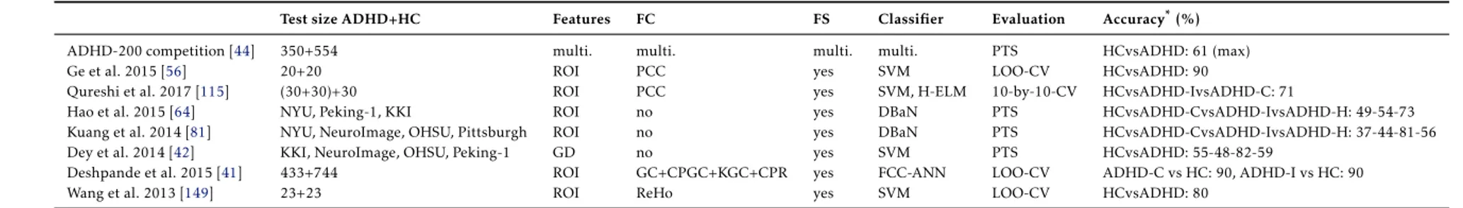
3 Literature Review 29 3.1 Classification of subjects in the ADHD-200 and Addiction Connectome Preprocessed Initiative (ACPI) databases . . . 30

3.2 Comparison of Statistical Methods for Brain Connectivity Estimation . . 33

3.3 Impact of Feature Selection in Neuroscience . . . 34

4 Materials and Methods 37 4.1 ACPI database . . . 37

4.2 ADHD-200 database . . . 38

4.3 Connectivity Matrices. . . 39

4.4.1 Classification in the ACPI dataset . . . 42

4.4.2 Classification in the ADHD-200 datasets . . . 44

5 Feature Set and Classifier Analysis 47 5.1 Feature set . . . 48

5.2 Classifier . . . 50

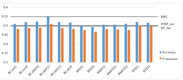
6 Results 55 6.1 Comparison of Methods . . . 56

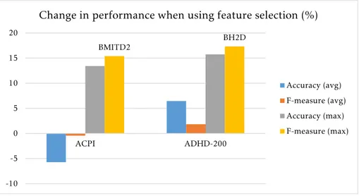
6.2 Feature Selection vs No Feature Selection. . . 57

6.3 Filtering vs No Filtering . . . 60

6.4 Single Matrix vs Multiple Matrices . . . 61

7 Discussion 67 7.1 Individual methods . . . 67

7.2 Impact of Feature Selection. . . 69

7.3 Impact of Filtering. . . 71

7.4 Combination of Matrices . . . 72

7.5 General Considerations . . . 74

8 Conclusions 77 Bibliography 79 I Results - Complementary Tables 93 I.1 Results in the ACPI dataset. . . 94

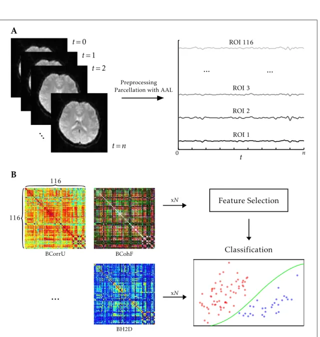
4.1 From rs-fMRI to classification . . . 46

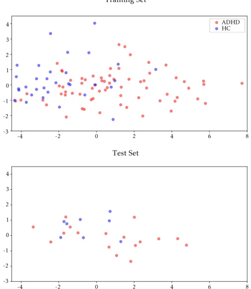
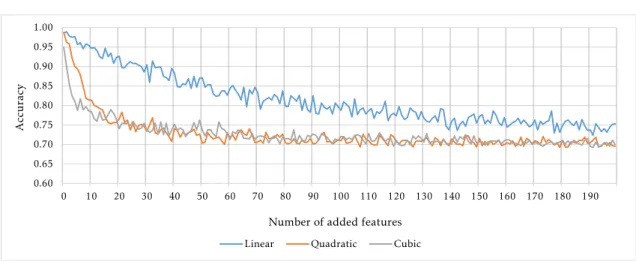
5.1 Most statistically significant feature in the ACPI and in the ADHD-200 filtered datasets . . . 49 5.2 Test and training set prior to classification in the ACPI dataset . . . 51 5.3 Accuracy as a function of the number of added features . . . 52

6.1 Classification performance in the ACPI dataset using a single connectivity matrix . . . 58 6.2 Classification performance in the ADHD-200 test sets using a single

connec-tivity matrix . . . 59 6.3 Change in performance caused by feature selection . . . 60 6.4 Change in performance caused by time series filtering . . . 61 6.5 Distribution of accuracy and macro-averaged f-measure values in

classifica-tions with a single matrix and with multiple matrices . . . 63 6.6 Macro-averaged f-measure performance as a function of the number of

2.1 Methods used to calculate FC and EC. . . 16

3.1 Summary of classifications using rs-fMRI in the ADHD-200 dataset. . . 32

4.1 Parameter values for every method available in MULAN following the termi-nology in [97, 147]. . . 41

6.1 Used methods and their notation. . . 56

I.1 5-fold CV with an RF classifier. . . 94

I.2 LOO CV with an RF classifier . . . 95

I.3 5-fold CV with an SVM classifier and without feature selection . . . 96

I.4 LOO CV with an SVM classifier and without feature selection . . . 97

I.5 5-fold CV with an SVM classifier and with feature selection . . . 98

I.6 LOO CV with an SVM classifier and with feature selection . . . 99

I.7 RF classifier in the validation set . . . 100

I.8 RF classifier in the test set . . . 101

I.9 SVM classifier in the validation set without feature selection . . . 102

I.10 SVM classifier in the test set without feature selection . . . 103

I.11 SVM classifier in the validation set with feature selection . . . 104

I.12 SVM classifier in the test set with feature selection . . . 105

I.13 RF classifier in the filtered validation set . . . 106

I.14 RF classifier in the filtered test set . . . 107

I.15 SVM classifier in the filtered validation set without feature selection . . . 108

I.16 SVM classifier in the filtered test set without feature selection . . . 109

I.17 SVM classifier in the filtered validation set with feature selection . . . 110

AAL Automated Anatomical Labeling.

ACPI Addiction Connectome Preprocessed Initiative. AD Alzheimer’s Disease.

ADC Apparent Diff_{usion Coe}ffi_cient.

ADHD Attention-Deficit/Hyperactivity Disorder. ANN Artificial Neural Network.

ANOVA Analysis of Variance.

ANTs Advanced Normalization Tools. AUC Area Under the Curve.

BOLD Blood-Oxygen-Level-Dependent.

C-PAC Configurable Pipeline for the Analysis of Connectomes.

DCM Dynamic Causal Modelling. DL Deep Learning.

DTI Diff_{usion Tensor Imaging.}

EC Eff_{ective Connectivity.}

EEG Electroencephalography. EPI Echo Planar Imaging.

FC Functional Connectivity. FCC Fully Connected Cascade.

FCP 1000 Functional Connectomes Project. FID Free Induction Decay.

fMRI Functional Magnetic Resonance Imaging. FN False Negatives.

FPR False Positive Rate.

HASTE Half-Fourier Acquisition Single-shot Turbo Spin Echo. HC Healthy Controls.

INDI International Neuroimaging Data-Sharing Initiative.

K-NN K-Nearest Neighbours.

LASSO Least Absolute Shrinkage and Selection Operator. LOO Leave-One-Out.

MDD Major Depressive Disorder. MEG Magnetoencephalography. MFC Most Frequent Class. ML Machine Learning.

MNI Montreal Neurological Institute. MRI Magnetic Resonance Imaging. MRMD Max Relevance Max Distance.

MTA 1 Multimodal Treatment of Attention Deficit Hyperactivity Disorder 1. MULAN Multiple Connectivity Analysis.

MVAR Multivariate Autoregressive.

OCD Obsessive-compulsive Disorder.

PCA Principal Component Analysis. PCP Preprocessed Connectomes Project. PET Positron Emission Tomography.

RBF Radial Basis Function. RF Random Forest.

ROC Receiver Operating Characteristics. ROI Region Of Interest.

ROIs Regions Of Interest. rs-fMRI resting-state fMRI.

SPECT Single-Photon Emission Computer Tomography. SVM Support Vector Machine.

C

h

a

p

t

e

1

I n t r o d u c t i o n

Since the mid 19th century, when Dr. John M. Harlow reported the now famous case of a man, Phineas Gage, that dramatically changed personality after surviving the destruction of his left frontal lobe provoked by an accident with an iron bar [65], that the human brain has been indubitably associated with cognitive function. Our knowledge of the brain and of its physiology has greatly increased since then, fast-forward one century and not only non-invasive techniques to anatomically image the brain and record its electrical activity had been developed but also techniques to image its functioning and activity over time. Despite that, years after the development of such techniques, we are still far from conquering the inherent complexity of said organ. We clearly can gather knowledge about the world around us but what we still do not know is how we/our brains do it.

Not too long after brain activity started being commonly recorded, it was hypothe-sised that if the activity from two neurons had a significant deviation from statistical independence, then, it could be that they were connected in some way [108]. This con-nection was then calledFunctional Connectivity (FC)[5]. This idea was generalized for populations of neurons and, in the early 1990s, the hypothesis that two brain regions could be functionally connected in individuals suff_{ering from neurological and}

psychi-atric disorders and in healthy subjects in diff_{erent ways was already established (e.g. [87]).}

In the same decade, the development ofFunctional Magnetic Resonance Imaging (fMRI) [13,104], which measures brain activity usingBlood-Oxygen-Level-Dependent (BOLD) contrast, greatly boosted research in this field and theFCbetween several brain regions of diff_{erent classes of subjects during a given task started to be explored. In the last decade,}

stored as matrices, calledFCmatrices.

Mental disorders are still currently defined and diagnosed mostly based on the inter-subject consistency of a set of personality traits and behavioural symptoms [10]. This diff_{use characteristic of psychiatry is not optimal and one would like to establish a more}

direct cause-disorder relationship. Thus, if diff_{erentFCpatterns are actually in the root}

of some mental disorders, the identification of such patterns could potentially provide new ways to define such disorders and greatly improve the diagnostic and prognostic tools of neurologists, psychiatrists and psychologists.

How would one identify group-diff_{erences in whole-brain connectivity patterns? That}

is whereMachine Learning (ML)techniques enter into scene. Automatic pattern recog-nition techniques have been developed long since and tasks such as this one are exactly the reason for which they are developed. Besides recognizing whether diff_{erences inFC}

patterns between groups of subjects actually exist, these techniques provide rules that can be used to classify a subject as belonging to one group or the other, in case the rule is true.

Several mathematical methods have been used to quantify theFCbetween two distinct brain regions, including correlation, the first one to be used, and coherence. Usually,FC patterns are derived using only one mathematical method to calculate theFCbetween a given brain region and all others.In this work, connectivity patterns are going to be derived using several mathematical methods simultaneously, and the separability of two classes using these patterns is going to be compared to the separability of the two same classes using patterns derived with only one mathematical method.

More specifically this study has four goals:

1. The first and main goal is to compare the classification performance of an ML classifier when using only oneFCmatrix to extract features, with its performance in the same conditions but using severalFCmatrices, each derived using a diff_erent

mathematical method, to extract features;

2. To investigate which statistical method derives theFCmatrix that yields the best classification performances;

3. To evaluate the impact of feature selection inFCbased classifications;

4. To confirm the importance of lowBOLDsignal oscillations (<0.1 Hz) in such clas-sifications.

need for betterADHDclassification methodologies than the ones currently in practice. Also, each mathematical method highlights diff_{erent relationships among brain activity}

signals, which means that significantly better classification performances using a specific method or a combination of them, could give insight on which relationships between diff_{erent regions actually reflect the biological causes behind the mental disorder in}

anal-ysis.

The remaining of this text is structured as follows:

Chapter2is intended to introduce the reader to the main concepts used in the follow-ing text, while developfollow-ing them to an extent that could ideally allow him/her to derive their own conclusions from the reported results.

Chapter3provides the state-of-art in classification of subjects withADHD, specifi-cally in the two databases used in this study, as well as the best available answers to the questions this study is intended to approach.

Chapter4thoroughly explains the methodology used to achieve the previously men-tioned goals in such a manner that the interested reader could closely replicate this study. Chapter5briefly analyses the separability of the two classes in order to evaluate the feasibility of the classifications and if the classification pipeline works properly.

Chapter6reports the results achieved using the methodology described in Chapter4 and their analysis.

Chapter7discusses the achieved results, compares them with what was hypothesised using the knowledge from Chapters2and3and provides the author’s thoughts on the results of those comparisons.

C

h

a

p

t

e

2

T h e o r e t i c a l Ba c k g r o u n d

The present Chapter is intended to introduce the reader to key concepts needed to un-derstand the following text. By the end of the Chapter, it should be clear how one can try to automatically distinguish two or more groups of people with diff_{erent neurological}

characteristics using brain activity. The reader is expected to be more or less acquainted withMagnetic Resonance Imaging (MRI), one of the most important techniques used to inspect the brain through bone and tissue and the one that originated the data used in this work. Notwithstanding, a very short introduction toMRIis going to be made next and, the remaining of the Chapter will be built on that.

2.1 Imaging the Brain

2.1.1 Magnetic Resonance

Let us consider a sample of an element in a constant magnetic field , B~0, with a given intensity and direction. If the nucleus of that element has non-zero spin, then it is going to acquire a precession movement around a rotation axis with the same direction of

~

B0, as a consequence of the torque applied by the magnetic field [128, pp. 209-211]. Additionally, in that case, the nuclear magnetic dipole moment of the element’s atoms might be oriented, relative to B~0, in a finite number of ways, depending on the spin magnetic moment of the nucleus [80, p. 398]. Each of these orientations corresponds to a given potential energy and, at low enough temperatures, the privileged one is that with the lowest energy. So, when a non-zero spin nucleus is put in an external magnetic field, its magnetic dipole moment precesses around the magnetic field and its energy varies depending on the acquired orientation. This energy split is what is commonly referred to as the Zeeman eff_{ect [80, p. 398].}

(both12C and 16O nuclei have null spin [30]) such that, to a first approximation, one can consider only the eff_{ect of the}1_{H nuclei, when analysing the e}ff_{ect of an external}

magnetic field on the body [24, p. 3]. The component of the magnetic dipole moment of a proton, the nucleus of a1H atom, codirectional to an external field similar toB~0, can be either±1/2 in~_{units, which means that they can only have two orientations and,} corre-spondingly, two energy levels in that case [128, pp. 206-208]. The distribution of protons between these two energy levels depends on the thermal energy and on the intensity of the external magnetic field [84, pp. 284-300]. The energy gap,∆_E, between the two

lev-els, corresponds to the energy of a photon with a frequency equal to the magnetic dipole moment precession frequency, commonly referred to as Larmor frequency orω0[128, pp. 211-212]. When an alternate magnetic field with frequencyω0, varying perpendicularly toB~0, is put over the precessing protons, these start to precess in phase with each other and with the field. Also, at the same time, some protons in the lowest energy level absorb an energy equal to the energy gap and pass to the highest energy level, changing their orientation to one regularly called “anti-parallel” to the constant external magnetic field (as opposed to the lowest energy level orientation, parallel to the same field)[128, p. 212]. This phenomenon of energy absorption when the two frequencies, the one from the al-ternate external magnetic field and the one from the precession movement, are equal, is called magnetic resonance [112].

2.1.2 Magnetic Resonance Imaging

It was previously said that if one puts an alternate magnetic field perpendicular toB~0 over the system constituted by the body plus the external constant magnetic field, some protons would change to the highest energy level. In the same way, when that alternate magnetic field is turned off_{, the distribution of protons between the two levels of energy,}

goes to a new equilibrium state. This new state might be similar to the one the system was in before the alternate field was turned on, if every other variable remained unchanged. Also, the precession phases of each proton will distribute randomly as before [24, pp. 8-9]. The variation in the magnetic field of the system caused by this proton relaxation, induces a current proportional to it. The intensity of the measured signal and its decay pattern reflect the type of tissue in analysis. For instance, if a given tissue has a higher proton density, the intensity of the measured signal is also going to be higher [128, p.214].

As explained, it is possible to distinguish diff_{erent types of tissue using the}

phe-nomenon of magnetic resonance. The gap between that and imaging is spatial encoding. For instance, let us consider a phantom with fragments of diff_{erent proton densities}

that is by using gradient magnetic fields [128, pp. 223]. Since the Larmor frequency is a function of the intensity of the magnetic field over the sample [24, p. 2], a gradient field introduces a spatial dependence to the equation. Because of the way the spatial encoding is made, the relaxation pattern (theFree Induction Decay (FID)signal) can be directly stored in the spatial frequencies space, or as it is also called in this case, the k-space. The information can, then, be converted to the image space using the inverse 2D Fourier transform [128, pp. 229-231].

Various alternate magnetic field pulses are usually needed for k-space to be com-pletely covered, however, in detriment of some image resolution, faster acquisition tech-niques have been developed as theHalf-Fourier Acquisition Single-shot Turbo Spin Echo (HASTE)imaging or theEcho Planar Imaging (EPI)[45].

2.1.3 Functional Magnetic Resonance Imaging

The variation of the magnetic resonance signal with the physicochemical properties of the medium and its short acquisition time, allow this type of medical image to be used for functional imaging. TheBOLDtechnique is the most commonly used forfMRIand it is based on the dependence of theFIDsignal on the blood concentration of deoxyhe-moglobin [104], that, due to it being a paramagnetic molecule, introduces a hypointense contrast in the MRI image [72, pp. 193].

The increase in metabolic activity in a given brain region, increases oxygen consump-tionin loco. This, in turn, increases the blood concentration of deoxyhemoglobin, leading to a rapid decrease of the magnetic resonance signal in the same area. The relative hy-poxia in the activated region, originates a local increase in blood supply, decreasing the concentration of deoxyhemoglobin, causing a lasting increase of intensity in theMRI im-age [72, pp. 193-199]. Thus, while imaging the brain, one could associate its hyperintense areas with their previous activation. The variations of theBOLDsignal are very small, which leads to a very lowSignal to Noise Ratio (SNR). To overcome this, cyclic activation patterns are induced by cyclic stimulation patterns which enables researchers to average out part of the noise. Nonetheless, lowSNRs are still one of the fundamental obstacles to the introduction offMRIin clinical practice [49].

Brain activity at rest was sometimes considered as uninteresting information [48]. Recently, however, it has been brought to the spotlight, particularlly since the discovery of valuable activity patterns such as the Default Mode Network, which is linked to intro-spection [62]. TofMRIusingBOLDcontrast while the patient is at rest one usually calls rs-fMRI[49]. This type offMRI, besides having a betterSNR[49], has the benefit of being a passive medical exam with minimal patient collaboration [48]. Such a characteristic widens the target population to patients with physical or neurological disabilities that do not allow them to cooperate as needed for task-relatedfMRIexams.

resolution [72, p. 202]. From thefMRI data and, particularly, from that acquired in a resting state, it is possible to evaluate the brain connectivity of a subject, something to be developed in the following Section of this Chapter.

2.2 Brain Connectivity

2.2.1 Structural Connectivity and the Connectome

The human brain is widely recognized as the most complex organ in our bodies and can surely be considered one of the most complex systems in the so far known Universe. Neurons are one of the structural units of the brain and the nervous system. They can receive, propagate and transmit stimuli, and together they form an ever changing neural network. The path a stimulus travels inside the neural network, as well as the biological action it triggers, depend on how that network is arranged i.e. on the neuronal pattern of connections, something defined as thestructural connectivityof the brain, also called anatomical or neuroanatomical connectivity.

There is a concept associated with structural connectivity on which great expectations of it becoming an unprecedented tool to understand the processes behind cognition are being deposited. This concept is called theconnectome. The connectome is a wiring map where every connection each neuron makes with the others is represented, with the goal of making a complete description of the structural connectivity of an organism [132]. Up to now, only one connectome has been completed, that of a nematode of the C. elegans

species. There are, however, projects aiming at storing and sharing human structural connectivity data of that type [46,133].

Currently, whole-brain structural connectivity of the human brain is understood mainly on the basis of the connections that white matter tracts establish between brain regions [131]. Because the diff_{usion of protons is anisotropic in such structures, these can}

be reconstructed usingDiff_{usion Tensor Imaging (DTI)which is anMRItechnique that} uses as contrast the diff_{usion coe}ffi_{cient of protons in the tissues (or, in fact, theApparent}

Diff_{usion Coe}ffi_{cient (ADC)) [96].}

2.2.2 Functional and Eff_{ective Connectivity}

Besides the physical connections between neurons or populations of neurons that di-rectly give rise to structural connectivity, another concept linked with brain connectivity emerged from the analysis of its activation patterns. This concept, called FC, aims at measuring how diff_{erent brain regions combine to perform a given task or thought,}

Another concept still not always objectively defined is that ofEffective Connectivity (EC) [127]. The distinction and relationship between ECandFC has not always been clearly stated, which has led to some diff_{erent interpretations of its definition within the}

neuroscience community. In an attempt to define these two concepts as coherently as possible, the definition ofECadopted here is also going to be based on the one given in the same paper by Friston. Having that into account,ECmight be defined as the influence a population of neurons exerts over another, measured on a statistical level [54].

The most important distinction betweenFCandECresides in the nature of the rela-tionships between the neuronal populations they aim to quantify, being non-causal in the case ofFCand causal in the case ofEC(here causal relationship should be understood in the context of Wiener’s definition [152]). Thus, measures ofECneed to be directed i.e. the measure ofECbetween two regionsX andY needs to be able to attribute diff_erent

values to the relationshipX →Y andY →X. There is a multitude of methods available to measure the statistical dependence between neurological signals, some to be introduced in the next Section, and, for some statistical metrics,ECmight be derived fromFC. The signals used to calculate both connectivity types might come from Electroencephalog-raphy (EEG),Magnetoencephalography (MEG),fMRIorPositron Emission Tomography (PET)data. Due to their better temporal resolution,EEGandMEGare the preferential brain activity recording modalities for the determination ofFCandEC.

2.2.3 Statistical Methods to Evaluate Functional and Eff_{ective Connectivity}

The scientific field responsible for the study of statistical dependences between two dif-ferent signals, having or not into account the influence of others, is multivariate statistics. Up to now, several methods from multivariate statistics have been applied to calculateFC andEC, each with its own origins and mathematical formulations. Taxonomically, these metrics can be divided into linear and non-linear, model based and model free, directed or non directed, based on time-domain representations or based on frequency-domain representations.

Cross-correlation and Pearson Correlation

Correlation is the most classical way of measuring the dependence between two neurolog-ical signals. Even today, the overwhelming majority of published studies in neuroscience use it as a measure ofFC[54] so much so that even the definition ofFCof some authors rests on the concept of correlation (e.g. [47]).

Letxnandynbe two random variables withn= 1, ..., N. Thecross-correlationfunction

betweenxnandynis defined as:

R_xy(τ) =E[x_ny_n+τ] =

1

N−τ N−τ X

k=1

This function measures how linearly dependent the two variables are. If the maximum value happens for a givenτ then one might establish a causal relationship between the two, even though this is not true for all cases. If the two variables are centred to zero and standardised by subtracting their respective averages and dividing next by their respective standard deviations, such that both xn and yn have zero average and unit

variance, thenRxy ranges between−1 (when one varies linearly with the symmetric of

the other) and 1 (when one varies linearly with the other), being positive when the two variables have a direct dependence and negative when they have an inverse dependence. IfR_xy is zero, the two variables are linearly independent. By centring and standardising the variables, the cross-correlation function actually becomes a standardised covariance function. In this context, thePearson product-moment correlation coefficient,r, is defined as the value of the centred and standardised cross-correlation function at zero lag (τ= 0):

r=

P

N(xn−x¯)(yn−y¯) pP

N(xn−x¯)2PN(yn−y¯)2

(2.2)

As shown by Rodgers and Nicewander in their paper from 1988, the Pearson coeffi

-cient can also be geometrically seen as the slope of the regression line between the two standardised variables [117].

Fourier Based and Wavelet Based Coherence

N. Wiener and A. I. Khinchine demostrated that the Fourier transform of the auto-and cross-correlation functions between two stationary rauto-andom processes, {xk(t)} and

{yk(t)}, where k is the index of the sample space, gives their auto- and cross-spectral

density functions, respectively, if the auto- and cross-correlations functions exist and their integral is finite [17, p. 199]. The relationships between these functions are, thus, also known as the Wiener-Khinchine relations. Mathematically, the spectral density functions can be expressed as:

Sxx(ω) = Z ∞

−∞

Rxx(τ)e−i2πωτdτ (2.3)

S_yy(ω) =

Z ∞

−∞

R_yy(τ)e−i2πωτ_{dτ (2.4)}

S_xy(ω) =

Z ∞

−∞

R_xy(τ)e−i2πωτdτ (2.5)

TheCoherenceorMagnitude Squared Coherencefunction can be defined as the normal-ized magnitude of the cross-spectral density function. Mathematically it can be written as:

cohxy(ω) =

|S_xy(ω)|

h

S_xx(ω)·S_yy(ω)i1/2

From equation2.6one can conclude that the coherence is a real-valued metric, func-tion of the frequency,ω. Coherence measures the linear dependency between two random processes for a given frequency, and ranges between 0 and 1, being zero for two linearly independent random processes and 1 in the opposite case. In spite of being real-valued, coherence is sensitive to both phase and magnitude [120], since its definition involves delaying the signals in respect to each other.

For finite length samples of two random variables, or for two diff_{erent signals, one}

can only estimate the spectral densities needed for the coherence expression. One way of doing this is by using the discrete Fourier (series) coeffi_{cients of the whole time window.}

This, however, does not yield a good estimate of the variables’ spectral densities [14]. One technique used to improve this estimation is the Welch’s method, which consists of dividing the whole time series in various temporal windows and then averaging their spectral density estimations. This, of course, only makes sense if the signals are stationary or close to being stationary because only in that case can we extrapolate the spectral characteristics of an entire signal from a given sub-sample of it.

In the particular case of event-related data, one can try to derive a better estimation by averaging the spectral densities over trials. Another alternative is to use a paramet-ric approach, where signals are considered, for instance, autoregressive processes [79]. Parametric approaches usually give good estimations but are computationally expensive, specially when compared to non-parametric methods such as the ones described above.

Because stationarity is not common in neural signals [83], an estimation of coherence over time should be considered. To achieve that, one can use wavelets to determine temporal estimations of spectral densities.

A wavelet is a function, usually represented by the symbolΨ_{, which satisfies certain}

mathematical criteria, such as having finite energy [3, p. 7]. Wavelets are localised in frequency and time and are used to transform signals to a representation dependent on these variables. There are several functions commonly used as wavelets but here the focus will be put on the complex Morlet wavelet, the most common one. Following [83], the Morlet wavelet can be defined for time,τ, and frequency,f, as:

ψ_τ,f(u) =p

f ei2πf(u−τ)_e−(u−τ)2

σ2 (2.7)

whereσ is the standard deviation of the Gaussian function defined by the third factor in equation 2.7, inversely proportional to the frequency, f. The Morlet wavelet can be seen as a complex sinusoid in a Guassian envelope. Both translation and dilation of the wavelet are possible by changing the values ofτ and σ respectively. The continuous wavelet transform of a signal,x, can be defined for any wavelet function,Ψ

x, as:

W_x(τ, f) =

Z ∞

−∞

x(u)Ψ

τ,f∗(u)du (2.8)

this case is equation2.7. This, however, is not always adopted by authors, being usual for these variables to appear only in the definition of the wavelet transform (e.g. [63]). Using the continuous wavelet transform one can compute the wavelet cross-spectral density between two signalsxandy, as:

SW_xy(t, f) =

Z t+δ/2

t−δ/2 Wx

(τ, f)W_y∗(τ, f)dτ (2.9)

whereδis a scalar. Using the Morlet wavelet, the cross-spectrum at a given frequency,f, is calculated for every time,t, using information within the interval [−δ/2 +t;δ/2 +t] with size (−δ/2 +t)−(δ/2 +t) =δ. This interval defines, thus, the temporal resolution of the wavelet. Within each interval the cross spectrum is determined in a very similar fashion to the temporal averaging described before, using a Gaussian as windowing function (see: [83]). The major diff_{erences lay on the variable width of both the Gaussian function and}

the intervalδ, the two inversely proportional to the frequencyf. For higher frequenciesδ

andσ decrease and the temporal resolution increases, for lower frequencies the opposite is true. The wavelet auto-spectrum density is calculated as in equation2.9but considering the transform and the conjugate of the same signal.

From the auto- and cross-spectral densities one can determine thewavelet coherence

between two signalsxandy, which can be written as:

W coh(t, f) = |SWxy(t, f)|

h

SW_xx(t, f)SW_yy(t, f)i1/2

(2.10)

Wavelet coherence also ranges between 0, when the two signals are linearly indepen-dent and 1, when the signals are linearly depenindepen-dent. When the two signals are linearly independent, however, coherence can be diff_{erent than 0. This happens because the}

esti-mation of the auto- and cross-spectral densities is not perfect and, because of that, neither is the estimation of coherence. When one intends to verify if two signals are linearly dependent, a statistical test should be used to compare, for instance, the obtained value of coherence with the distribution for two random independent signals. Similar statis-tical tests can be used when analysing the cross spectrum against a population specific background spectra, usually defined as the mean time-averaged wavelet power spectrum, as stated in [120].

Much more can be said about wavelet spectra and wavelet coherence. For more in-formation about the subject the interested reader is referenced, for instance, to [3, 83, 139].

Mutual Information

One of those metrics, based on concepts from information theory, is mutual information [124]. To define mutual information one should first introduce the concept of entropy. Historically, the entropy measure used for mutual information is the Shannon entropy [124]. Let us consider the histogram of a random variablexwithLbins. The probability,

p_ixof an occurrence ofxto fall in a given bini,i= 1,2, ..., L, might be simply defined as

p_ix=ni/N whereni is the previous number of occurrences that fell ini andN=PLi=1ni

is the total number of occurrences. Following that, the Shannon entropy ofxis given by [118]:

H(x) =−X

i∈L∗

p_ixlnp_ix (2.11)

whereL∗_{is the set of bins withn}

i,0.

The previous definition ofpx_i introduces an underestimation of entropy for a finite number of samples ofx whenp_ix= 0 [38]. To compensate for this, a corrected form of entropy might be defined following [118] as:

H∞(x) =H(x) +

|L∗_{| −1}

2N (2.12)

where| · |is the cardinality of the set. The Shannon entropy can be seen as the expected value of lnp_i. This leads to low entropies for “concentrated” distributions and high en-tropies for “spread” distributions. In fact, the entropy is maximum when the distribution ofxis uniform and zero when all occurrences are in the same bin. This happens because, for values smaller than 1, the negative of the logarithmic function favours lower values and greatly penalizes high values, so, if the distribution is spread, there will be more values close to zero and the entropy will be higher.

As was done for a single random variable, one can also define the entropy between two random variables,xandy. Consideringysegmented intoM bins andpy_j the probability of an occurrence ofyto fall inj, the joint entropy betweenxandyis given by:

H(x, y) =−X

i∈L∗

X

j∈M∗

p_ijxylnpxy_ij (2.13)

wherep_ijxy=nij/N withnij being the number of occurrences ofx ini, when y falls inj.

Using the joint entropy one can define themutual informationbetweenxandyas:

MI(x, y) =H(x) +H(y)−H(x, y) =X

i∈L∗

X

j∈M∗

p_ijxyln p

xy ij

px_ip_jy (2.14)

again, following [118], one correction to2.14is:

MI∞(x, y) =MI(x, y) +

|L∗_|+|M∗_{| − |LM}∗_{|+ 1}

2N (2.15)

whereLM∗_{is the set of pairs of bins that satisfyn}

Equation2.14allows us to understand what mutual information is actually measuring. Ifx andy are independent, thenpxy_ij =px_ip_jy andH(x, y) =H(x) +H(y), which results in

MI = 0. Thus, mutual information is always greater or equal than zero and measures the diff_{erence between the joint entropy when one assumes the two variables as independent}

and the actual joint entropy. When the two variables are similarMI has its maximum value and if the two variables are commuted the result is the same (MI(x, y) =MI(y, x) because H(x, y) =H(y, x)), which means thatMI gives no information about causality. One way to introduce directionality (and hence possibly causality) in mutual information is to introduce a time lag in one of the variables and calculate equation2.14for diff_erent

lags [144].

Transfer Entropy

Delayed mutual information does give us information about direction, but there is, how-ever, another statistical method, also based on information theory, that was defined specif-ically to measure the flow of information. This measure, called transfer entropy, was introduced by Thomas Schreiber in 2000 [121]. Transfer entropy is based on the concepts of transition probability and entropy rate. If a time seriesx can be approximated by a stationary Markov process of orderkthen the time-conditional probability of findingx

in the state (or the bin, if we are still looking at the variable’s histogram)in+1at timen+ 1 is independent of the statein−k. The entropy rate ofx, then, measures how much entropy xhas, given the knowledge of its previouskstates. Mathematically, the entropy rate ofx

can be expressed as:

Hrate(x) =− X

in+1,...,in−k+1

px(in+1, ..., in−k+1) lnpx(in+1|in, ...in−k+1) (2.16)

Both mutual information and transfer entropy can be understood in the context of the Kullback entropy [82], which might be expressed, for a given variable, as K =

P

ipx(i) lnpx(i)/qx(i) whereq(i) is the assumed probability distribution andpx(i) the

ac-tual probability distribution. The Kullback entropy measures the error of assuming the wrong probability distributionqx(i). Mutual information can, thus, be seen as the joint Kullback entropy between two variablesxandy, when assuming the two variables inde-pendent or, mathematically, assuming thatqxy_{(i, j) =p}x_(i)py_{(j). Transfer entropy shall be}

here defined too in the context of the Kullback entropy as Schreiber did in his paper. Let us consider the following Markov property:

px(in+1|in, ...in−k+1) =pxy(in+1|in, ..., in−k+1, jn, ..., jn−l+1) (2.17)

T E_y→x=

X

in+1,...,in−k+1,jn,...,jn−k+1

pxy(i_n+1, in(k), jn(l)) lnp xy_(i

n+1|in(k), jn(l)) px_(i

n+1|in(k))

(2.18)

whereinandjnare, as before, the possible states of, respectively,xandyat timen. Also, a

shorthand notationin(k)= (in, ..., in−k+1) andjn(k)= (jn, ..., jn−k+1) was here used as introduced by Schreiber.

By measuring the deviation from property2.17, transfer entropy attempts to measure the information theory equivalent of Wiener’s causality. Thus, transfer entropy not only is a directed measure, but also a model-free candidate to measureEC. For more information on transfer entropy and its applications to neuroscience the reader is referred to [145, 151].

Non Linear Correlation Coeffi_cient

In 1989 Lopes da Silva et al. [89] first used the non linear correlation coeffi_{cient to}

mea-sure the relationship betweenEEGsignals. The idea behind this coeffi_{cient is to consider}

a given dependent variable, yn, of finite lengthN as a function of another variable, xn,

and calculate the fraction of the total variance ofy_n that can be explained byx_n. This measure is called η2and to estimate it one can use the regression curve to estimatey_n

fromxn and calculate the unexplained variance ofyn using the estimation errors. The

explained variance ofy_nis then calculated by subtracting the unexplained variance from the total variance. The estimation ofη2is symbolized byh2.

To approximate the regression curve without assuming any relationship between the two variables, a piecewise linear regression is commonly used. In particular, Lopes da Silva et al. referred to a piecewise approximation of the regression curve by partitioning the independent variable,x_n, intoLbins and connecting the points (y_n,i, x_n,i|_mid) in the scatter plot ofyn as a function of xn, whereyn,i is the average value ofyn in bini and xn,i|midis the midpoint ofxnin bini. Let the function ˆyn(xn) be the estimation ofynfrom x_n. The non linear correlation coeffi_{cient betweenxnandynis calculated as:}

h2_xy=

P

N(yn−yn)2−PN(yn−yˆn(xn))2 P

N(yn−yn)2

(2.19)

The non linear correlation coeffi_{cient ranges between 0, when the two variables are}

independent, and 1 when one is completely determined by the other. Also, it is a sym-metric measure if the relationship between the two signals is linear and asymsym-metric, i.e.

h2_xy ,h2yx, otherwise. Also, one can calculateh2xy for different lags ofyn and conclude a

possible causal relationship using the lag that maximizes the coeffi_cient.

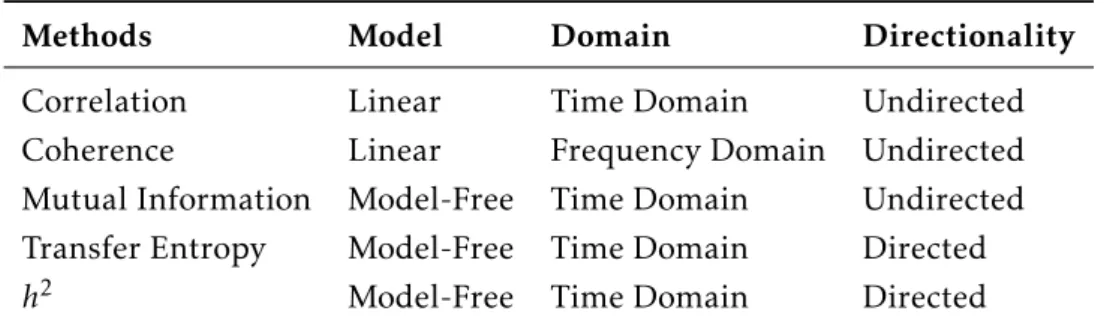
Table 2.1: Methods used to calculate FC and EC.

Methods Model Domain Directionality

Correlation Linear Time Domain Undirected

Coherence Linear Frequency Domain Undirected Mutual Information Model-Free Time Domain Undirected Transfer Entropy Model-Free Time Domain Directed

h2 Model-Free Time Domain Directed

brain connectivity is the possibility of extrapolating from it a method for measuring its value between two neurological signals while controlling for the others, eff_ectively

avoiding spurious dependencies that come from a simultaneous dependency on other neurological signals, a characteristic only some possess.

Studies using linear methods still greatly outnumber the ones using non-linear meth-ods1and a number of reasons can be associated with that. The diff_{erence between the}

number of available tools to measure each method, which is much higher for linear meth-ods, might be one of the reasons. It might also be for comparison purposes or historical reasons. In addition, linear methods are less complex and have been associated with better robustness to noise (for a brief review on this matter see [20]).

From image acquisition to the determination of brain connectivity some steps might come into place to organise, spatially label or reduce the amount of information to be dealt with. The next Section will briefly cover this matter.

2.2.4 Image Registration and Brain Parcellation

Every brain is diff_{erent. While some might be reasonably similar, others, like the ones}

from adults and children, are quite distinct. Due to this variability, defining regions in the brain is not as easy as applying the same three dimensional mask on every brain. Besides inter-subject variability, imaging techniques such has fMRI have low image resolution which hinders the identification of some brain constituents. Eff_{orts to solve both these}

issues have been boosted in recent years by the fast increase in computational power andin vivoimaging techniques. Furthermore, not only is a consistent method needed to define regions in the brain, but the regions should also not be defined randomly. Image registration in a standard space and parcellation with brain atlases are two common preprocessing steps used to diminish anatomical variability and to consistently define meaningful brain regions.

1_{A search on PUBMED for papers using linear correlation as a connectivity measure was made with the}

terms: (“brain connectivity” OR “functional connectivity”) AND (correlation OR cross-correlation) NOT (“non-linear correlation” OR “non linear correlation”) revealed 325 results in 2016 while a search for papers using non-linear methods to measure connectivity with the terms: (“brain connectivity” OR “functional connectivity” OR “eff_{ective connectivity”) AND (“Granger causality” OR “mutual information” OR “transfer}

Image registration is made, for instance, using an algorithm that iteratively applies a transformation model to an anatomical or a functional image (the source or moving image) until a specific threshold of correspondence with a reference (or fixed) image is met [58]. Registration of brain images is usually made into a standard high resolution brain template or atlas to allow not only functional localisation but also comparison between subjects, by diminishing the inter-subject brain anatomy variability. Some brain atlases automatically label diff_{erent regions of the brain, such as the widely knownAutomated}

Anatomical Labeling (AAL)atlas [141] which defines 116 regions. In this study, what interests us mostly is what the common practice infMRIdata is and as such, we shall now focus on image registration and brain parcellation of fMRI volumetric data. For general information on brain atlases, templates and their associated image and volume registration techniques, the reader is referred to e.g. [58,143].

As previously stated, functional imaging, whether fromfMRI,PETorSingle-Photon Emission Computer Tomography (SPECT), deals at a fundamental level with the trade-off _{between temporal and spatial resolutions. Image registration relies on the quality}

of the source image for an accurate identification of the features needed to analyse its correspondence with the reference image. Because of the temporal resolution needed for functional imaging, and particularly forfMRI, the spatial resolution of these techniques does not serve this purpose in most cases. Nonetheless, functional to anatomical regis-tration i.e. regisregis-tration of a subject’s functional image to his corresponding anatomical image, can still be accurately made because both images represent the same anatomical structure. Taking advantage of this, functional to template or atlas registration is possi-ble by registering the functional images of interest to an anatomical image of the same brain and afterwards by applying the transformations needed to pass the high-resolution anatomical image to the wanted template or atlas, to those functional images [59]. Once registered to an atlas, or to an atlas space, thefMRIvolumes become eff_{ectively parcelated}

or ready to be parcellated.

ForFCorECstudies, the brain should ideally be parcellated in such a way that the time series of each voxel somewhat represents the general activation pattern [154] or the FCpatterns [33] of the region in which it is included. Because every subject has its own activity and connectivity patterns, constructing an atlas based on this criterion is not an easy task, but some attempts have been made e.g. [37]. When using the statistical methods mentioned in Section2.2.2, calculating the dependencies between the time series of every voxel of the brain in thefMRIvolume can be computationally expensive. Thus, combining the time series of each region’s voxels is a way of eff_{ectively diminishing the}

dimensionality of the data and, therefore, the computational cost of the process. Typically, the time series of each region is determined by averaging the time series of every voxel that constitutes it.

series of eachRegion Of Interest (ROI)can, then, be extracted by voxel-wise time series averaging and the subject’s brain connectivity determined by calculating the statistical dependencies between each extracted ROI with a given multivariate analysis method. Thus, if a brain is constituted by n voxels in a givenfMRI volume and the used atlas hasmROIs, after time series extraction for eachROIwe pass from n, tom time series. The dependency values between allntime series (n×nvalues to be calculated) can be organized in a matrix, calledFCmatrix. Thus, by extracting a single time series for each ROI, the number of dependency values to be calculated is reduced byn2−m2values.

Even under the same conditions, each person has its own structural and connectiv-ity patterns and one of the paradigms in neuroscience is to find a way of using this information to find consistent diff_{erences between groups of subjects, that would allow}

technicians to use these techniques for diagnostic and prognostic of neurological diseases. One possible technique that can be used to find group diff_{erences in the patterns of brain}

connectivity isML.

2.3 Machine Learning

In many ways computers are like brains, both are systems that constantly receive input stimuli, convert them into electrical signals and process that information for storage and/or to produce an output. Despite their similarities, one area in which brains and computers are still quite diff_{erent, is in the process of using the information they receive}

as experience to learn something new. ML can be described as the area of computer science responsible for making methods capable of detecting patterns in data and use them as experience to make future predictions [99, pp. 1-2].

Learning can be supervised, unsupervised, semisupervised or by reinforcement. In this text the first two types are going to be briefly described but the focus will fall mostly on the first. What distinguishes the type of learning is how the learning set, or the training set data is presented to the implemented algorithm. For supervised learning, the sample is given as a pair{x_i, yi}, i = 1, ..., N ,xi∈RnwhereNis the number of data points,

2.3.1 Supervised Machine Learning Algorithms

Classification tasks generally have the same work-flow: data gathering, assembly of repre-sentative training, validation and test sets, choosing a learning algorithm for classification, parameter tuning in the validation set and finally model evaluation in the test set. Several algorithms can be used for supervised learning, some are instance based e.g. K-Nearest Neighbours (K-NN)[85], others are model based e.g. logistic regression [99, pp. 21-22]. In neuroscience,Support Vector Machine (SVM)[35] andDeep Learning (DL)algorithms are commonly used for classification and regression tasks (see for instance [90, 130]). Even though DL is of great interest for neuroscience, in this text it is not going to be covered because it was not used in this study. For a review of DLsee e.g. [86] or for a book e.g. [60]. Next,SVMs are going to be introduced as well as ensembles of decision trees, which have been applied with success in classification tasks.

Support Vector Machines

In 1995, Cortes and Vapnik [35] introduced a new supervised and model based learning algorithm which draws linear decision boundaries based on the so called large margin principle. It was introduced for two class classification problems but has since been generalized to multiclass and regression problems, however, here it is only going to be considered the two class case. This algorithm was then called support vector networks

by the authors and is now referred to asSVM. The previously mentioned large margin principle states that, of all decision boundaries that linearly separate two classes in the feature space, the best is the one that maximizes the margin between the boundary and the closest point to it, i.e., the one that maximizes the distance, r, to the closest point, measured orthogonally from the boundary defined by the discriminant function [99, p. 501].

In model based supervised learning, the discriminant function is a function, say

f(x_i, α), whereα are its free parameters, that maps the values in the feature space to estimated label values: ˆy_i=f(x_i, α). The ultimate goal is to find the values ofαfor which

f(x_i, α) maps every data point to the correct label, while providing a good generalization to new data points. For two class classification, the sign of the discriminant function decides on which side of the boundary each data point stands (positive value corresponds to a given label and a negative value to the other label; the decision boundary is defined by f(x_i, α) = 0). As previously said, in anSVM algorithm, the discriminant function is linear f(x) =wT ·x+b, where w is a vector normal to the hyperplane andb is the translation constant that controls the distance from the hyperplane to the origin. In this algorithm, the discriminant function should not only correctly map every point, but also, following the large margin principle2_{, draw a decision boundary that maximizes r or,}

2_{For the sake of clarity, the margin of the decision boundary is the set of points of the input feature space}

diff_{erently put, that minimizeskwkgiven thatr=f(x)/kwk. If we assumeyi= 1∨yi=−1}

andysf(xs) = 1, wheresis the index of the data point closest to the decision boundary,

we can mathematically express the initial objective of theSVMalgorithm as [25]:

min

w,b

1

2kwk2 s.t. yi(wT ·xi+b)≥1∀i (2.20) The minimization is on 1₂kwk2and not on kwkto simplify the derivative, which be-comes justw, and to make it diff_{erentiable atw= 0 [57, pp. 145-165]. The data points}

that define the largest margin size are calledsupport vectorsand are the ones with index

s, for which the equality in2.20holds.

There are two problems with an algorithm that only applies the large margin principle to a linear discriminant function, while having the correct value ofsign{f(x_i)}for every

x_i. The first problem is that most classes are not linearly separable. In such cases, the constraint imposed on the sign off(x_i) yields no solutions to the minimization problem (the constraint is never satisfied). To overcome this, Cortes and Vapnik introduced a slack variable,ξi, that measures how muchxican violate the pre-defined margin. In the

previ-ous binary context,ξ_i= 0 ifx_i is on the correct margin boundary or outside the margin but on the correct side of the decision boundary andξ_i=|y_i−f(x_i)|otherwise [99, p. 501]. The objective is now to minimize 1₂kwk2and the margin violations, mathematically:

min

w,b,ξ

1 2kwk

2_+CXN

i=1

ξ_i s.t. ξ_i≥0, y_i(wT·x_i+b)≥1−ξ_i (2.21)

whereC is a constant.

The construction of the optimal hyperplanes is a convex quadratic programming problem [35] and the steps to its solution are not going to be covered here.

It was said that there were two problems with the mentioned algorithm, the first can be solved with the introduction of slack variables, but the discriminant function is still linear. To produce non-linear discriminant functions in the original feature space one might do a non-linear mapping ofx_ifrom the original feature space to a high dimensional feature space and solve equation2.21in that high dimensional space. Computationally, however, this process can be very expensive. One way of going around this issue is by using the so calledkernel trickin the corresponding Lagrangian dual problem which has the same solution of the primal problem (equation2.21) in the given conditions3_{. The}

dual problem can be shown to be [25]:

min α 1 2 N X i=1 N X j=1

αiαjyiyjxTi ·xj− N X

i=1

αi s.t. N X

i=1

αiyi= 0,0≤αi≤C, ∀i (2.22)

where αi and αj are the Lagrange multipliers. After finding the minimal α one can

calculatewminandbminusing [18, pp. 334-335]:

3_{The inequality constraints and the objective function are convex and the former are continuously di}ff

w_min=

N X

i=1

α_iminy_ix_i (2.23)

bmin= 1 |M_|

X

i∈M        

y_i−X

j∈S

α_jy_jxT_i ·x_j

        (2.24)

whereM is the set of indices of the data points that satisfy 0_{≤ αi ≤C}, Sis the set of indices that correspond to the support vectors, which in this case are the ones that satisfy

y_if(x_i) = 1−ξ_iand| · |is the cardinality of the set.

When using a mapping function, sayφ(x), the dot products in equations 2.22and 2.24can be replaced byφ(x_i)T_·φ(x

j). The kernel trick consists in using a Mercer kernel

function, κ(x_i,x_j), to calculate the dot product κ(x_i,x_j) =φ(x_i)T _·φ(x

j) only using the

original vectorsx_iandx_j [99, p. 481]. This means that even if the functionφ(x) maps to a very high dimensional space, the computational cost is similar to the linear case in the original feature space.

The polynomial and theRadial Basis Function (RBF) kernels are two examples of Mercer kernels. The former allows one to work with mapping functions that originate features by multiplying the original features with each other and the latter allows one to work with functions that map to infinite dimensional spaces [99, pp. 481-482]. RBF kernels are widely used inSVMalgorithms and consist of Gaussian kernels of the form:

κ(x_i,x_j) =e(−γSV Mkxi−xjk) 2

(2.25)

whereγSV M defines the width of the gaussian function.

It should be noted, lastly, that the determination of the discriminant function depends only on the support vectors and that its shape depends on the parameterC of function 2.21 and on the parameters of the kernel. HighC values result in fewer margin viola-tions but smaller margins and lowC values result in the opposite. Because the decision boundary only depends on the support vectors this algorithm is memory effi_{cient. Also,}

because of this, its performance might not be aff_{ected by the number of features [91].}

Ensembles of Decision Trees

Classification based on a decision tree is made as follows4. The most discriminant feature of the original feature set is estimated and used as the root of the tree, from where the classification starts. By looking at the values of the root feature for each class, a self-complementary set of equality and/or inequality rules is put together with the goal of separating the existing classes as well as possible, using only the root feature. The process of creating rules from a given feature is called branching because each rule is going to correspond to given branch of the tree. Based on the separation of instances motivated by

4_{To simplify the explanation, the text refers to non oblique decision trees, which means that each node}