Effect of Pressure dependent demand on
pipe network analysis: A case study
MINAKSHI SHRIVASTAVA
Maulana Azad National Institute of Technology Bhopal,462051,India
Dr. RUCHI KHARE
Maulana Azad National Institute of Technology Bhopal,462051 ,India
Dr. VISHNU PRASAD
Maulana Azad National Institute of Technology Bhopal,462051,India
Abstract :
Water distribution network is most important part of world’s infrastructure. In the present work, analysis for proposed site of school of planning and architecture, Bhopal is done by using demand based analysis and the design is further analyzed for pressure dependent demand. Detailed study of variation of threshold pressure with power function is carried out .Complete site is divided into two zones having two separate water tank for supply and the analysis is done by varying threshold pressure and power function in case of pressure dependent demand by using commercial pipe network analysis software.
Keywords: network analysis, pressure based analysis, demand based analysis, node, power function, threshold pressure.
1. Introduction:
It is the most common practice to design municipal water supply network adequate supply of water to the individuals at required pressure. Water supply network comprises different pipe and junctions. There are many conventional methods to analyze pipe network such as Hardy Cross method, Linear Theory method, Newton Raphson method, Finite Element method etc. All these methods are based on the two major laws. 1) It must satisfy the continuity equation i.e the amount of water entering to the junction must be equal to the amount of water leaving from the junction. 2) Net head loss within the loop must be zero. Hardy cross is the oldest and simplest method for pipe network analysis but it has very slow rate of convergence. This drawback was overcome in Newton Raphson method i.e. it has faster rate of convergence but in this method there is a need to evaluate each derivative of flow equation with respect to the rate of flow. Another method called linear theory method overcome this limitation. This method gives better accuracy in few iterations i.e. has very rapid convergence rate [1]. From the literature survey, it can be seen that demand based analysis is the most convenient method for pipe network analysis . But it can not supply required amount of water to the consumer in case of abnormality. i.e if some part of the network is closed for maintenance [3,7].
It is observed from literature review that if there is any abnormality in the network, the pressure at some of the junction reduces and not able to supply the required demand. For such situation pressure based analysis may be helpful for finding the actual demand to be supplied at the time of maintenance [2,3]. Different conventional and non conventional methods are used for pressure dependent analysis. Zheng Y. Wu et al [5] have worked on pressure dependent analysis of water distribution system by using global gradient algorithm. Wah Khim Ang [6] introduced another approach called pressure deficient network algorithm (PDNA).PDNA is incorporated with EPANET and analysis is done for both single and multiple source network.
2. Numerical formulation
Various commercial softwares are available in market to analyze and optimize the water supply network. Water Gems is one of the most effective software available in the market. It works on the law of conservations. The conservation of flow at each node is given as:
in out external
Q
Q
Q
………….………..(1)2.1 Threshold Pressure :- It is the minimum pressure required to supply the water demand at the
Junction. i.e. If the pressure at the junction is above the threshold pressure, it will not affect the demand.[3]
0
0
0
I
s
i
i t
ri ri
t
t i
ri
H
Q
H
H
H
Q
H
H
H
H
H
.………...………...(2)
3. Network modeling of SPA:
In present work design of water supply network is done for school of planning and architecture, Bhopal. The total area is divided in two zones as shown in figure 3. Zoning is done in such a way that head loss will be minimum and length and diameter of the pipe is selected to get minimum cost . Demand at each location is calculated using 2 hrs supply per day considering suitable demands [10]. The RL of the network is taken 1 m below the form work of the road network. Initially the demand based analysis was done for each network. For pressure dependent analysis , variation of threshold pressure for zone 1 is from 15 to 22 and power function varies from 0.5 to 0.8, for zone 2 threshold pressure varies from 13 to 21 and power function varies from 0.5 to 0.8,for both the cases reference pressure is taken as equal to the threshold pressure.
Fig.3: Pipe network layout of SPA, zone 1 and 2.
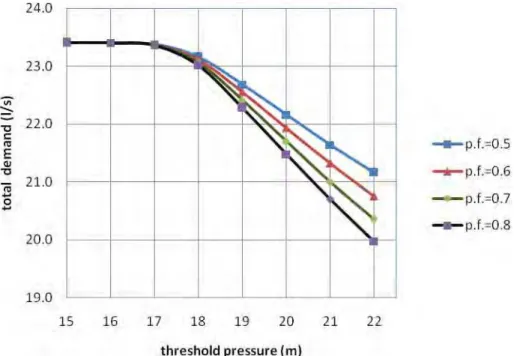
Fig 4: Variation of total demand with threshold pressure for zone 1
Fig.5: Variation of total demand with threshold pressure for zone 2
4.Results and Discussions:
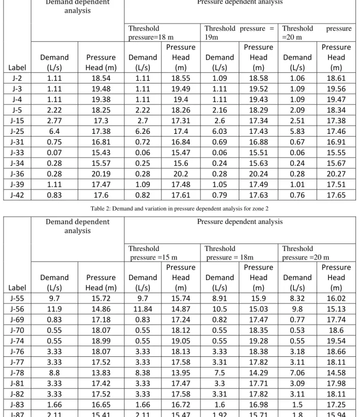
The comparison of demand and pressure head in cases of Demand dependent analysis and Pressure dependent analysis at some junctions of Zone I and Zone II is shown in Table 1 and 2. Which shows that demand is decreasing with increase in threshold pressure.
Table 1: Demand and pressure variation in pressure dependent analysis
Demand dependent
analysis Pressure dependent analysis
Threshold
pressure=18 m
Threshold pressure = 19m Threshold pressure =20 m Label Demand (L/s) Pressure Head (m)
Demand (L/s) Pressure Head (m) Demand (L/s) Pressure Head (m) Demand (L/s) Pressure Head (m) J‐2 1.11 18.54 1.11 18.55 1.09 18.58 1.06 18.61 J‐3 1.11 19.48 1.11 19.49 1.11 19.52 1.09 19.56 J‐4 1.11 19.38 1.11 19.4 1.11 19.43 1.09 19.47 J‐5 2.22 18.25 2.22 18.26 2.16 18.29 2.09 18.34 J‐15 2.77 17.3 2.7 17.31 2.6 17.34 2.51 17.38 J‐25 6.4 17.38 6.26 17.4 6.03 17.43 5.83 17.46 J‐31 0.75 16.81 0.72 16.84 0.69 16.88 0.67 16.91 J‐33 0.07 15.43 0.06 15.47 0.06 15.51 0.06 15.55 J‐34 0.28 15.57 0.25 15.6 0.24 15.63 0.24 15.67 J‐36 0.28 20.19 0.28 20.2 0.28 20.24 0.28 20.27 J‐39 1.11 17.47 1.09 17.48 1.05 17.49 1.01 17.51 J‐42 0.83 17.6 0.82 17.61 0.79 17.63 0.76 17.65
Table 2: Demand and variation in pressure dependent analysis for zone 2
Demand dependent
analysis Pressure dependent analysis
Threshold
pressure =15 m
Threshold pressure = 18m
Threshold pressure =20 m
Label
Demand (L/s)
Pressure Head (m)
Demand (L/s) Pressure Head (m) Demand (L/s) Pressure Head (m) Demand (L/s) Pressure Head (m) J‐55 9.7 15.72 9.7 15.74 8.91 15.9 8.32 16.02 J‐56 11.9 14.86 11.84 14.87 10.5 15.03 9.8 15.13 J‐69 0.83 17.18 0.83 17.24 0.82 17.47 0.77 17.74 J‐70 0.55 18.07 0.55 18.12 0.55 18.35 0.53 18.6 J‐74 0.55 18.99 0.55 19.05 0.55 19.28 0.55 19.54 J‐76 3.33 18.07 3.33 18.13 3.33 18.38 3.18 18.66 J‐77 3.33 17.52 3.33 17.58 3.31 17.82 3.11 18.11 J‐78 8.8 13.83 8.38 13.95 7.5 14.29 7.06 14.58 J‐81 3.33 17.42 3.33 17.47 3.3 17.71 3.09 17.98 J‐82 3.33 17.52 3.33 17.58 3.31 17.82 3.11 18.11 J‐83 1.66 16.65 1.66 16.72 1.6 16.98 1.5 17.25 J‐87 2.11 15.41 2.11 15.47 1.92 15.71 1.8 15.94
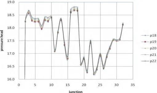
Fig. 6: Effect on pressure head at all junctions in zone 1 with the variation of threshold pressure
Fig. 7: Effect on pressure head at all junctions in zone 2 with the variation of threshold pressure
In fig 6, effect on pressure head with the variation of threshold pressure has been shown for zone 1 with power
function 0.7.P18 to P22 are the conditions where power function is 0.7 and threshold pressure varies from 18 m
to 22 m respectively.
It has been seen from the analysis that pressure head is same with that in case of demand driven analysis for threshold pressure less than 17 m. with the increase in threshold pressure, head variation can be seen in the above figure.
When the threshold pressure is less than the pressure at the junction, the supply will be less at that
point. and if the pressure is more than the threshold pressure, required amount of water will be supplied to the consumer.
It can be observed from the results that if threshold pressure is less than the junction pressure, actual
Fig. 7 shows the variation of pressure head with threshold pressure for zone 2 with power function 0.7. Z 21 to Z27 are the conditions where threshold pressure varies from 15m to 21 m for zone 2.
It can be observed from the analysis that for constant power function, head is not much affected by the
threshold pressure i.e. for less threshold pressure, head is almost constant. but for high threshold pressure, there is considerable change in pressure head.
Conclusion:
From the pressure based analysis it may be observed that the power function and threshold pressure are inter related to each other. Higher value of power function yields to steep change in total demand whereas the total demand is nearly independent of threshold pressure below 15 m. However it will also depend on the layout and demands at different nodes.
Notations :
Qin = flow into the node
Qout= flow coming out from the node.
Qexeternal = outside demand at the node.
Qs = calculated demand
Qri = required demand
Hi = Calculated pressure at node
Hri = Reference pressure
Ht = Threshold pressure
References:
[1] Gay B. and Middleton P. (1970) "The solution of pipe network problem ", Chemical engineering science, volume 26, pp. 109-123. [2] Do Guen Yoo, Min Yeol Suh, Joong Hoon Kim, Hwandon Jun and Gunhui Chung (2011) ” Subsystem based pressure dependent
demand analysis in water distribution system using effective supply ”, KSCE journal of civil engineering, volume 3,pp.457-464. [3] Zheng Yi Wu and Thomas Walski (2006)”Pressure dependent hydraulic modeling for water distribution system under abnormal
conditions”, IWA world water congress and exhibition, pp.1-11.
[4] Bently system, incorporated,(2005), water-gems user manual. 27 siemon co dr, suite 200W,watertown, CT06795,USA.
[5] Zhen Y. Wu, Rong H. Wang, Thomas M. Walski, Shao Y. Yang, Danniel Bowdler and Christopher C. Baggett(2009),”Extended global gradient algorithm for pressure dependent water distribution analysis”,Journal of water resources planning and management, volume 135,pp.13-22.
[6] Wah Khim Ang and Paul W. Jowitt (2006), ” Solution for water distribution system under pressure-deficient conditions”, Journal of water resources planning and management, volume 132,pp.175-182.
[7] Gupta Rajesh and Bhave Pramod R.(1996), ” Comparision of methods for predicting deficient-network performance”, Journal of water resources planning and management, volume 122, pp.214-217.
[8] Krope J., Dobersek D. and Goricanec D.(2000),”Flow pressure analysis of pipe network with linear theory method”,Proceedings of the WAEAS/IASME international conference on fluid mechanics,Miami,Florida, USA,pp. 59-62.
[9] Chun Woo Baek, Hwan Don Jun and Joong Hoon Kim(2009),”Development of a PDA model for water Distribution system using harmony search algorithm”, KSCE Journal of civil engineering, volume 14(4), pp.613-625.
[10] Manual on water supply and treatment, (1991) Published by central public health and environmental engineering organization,Ministry of urban development, Third edition.