www.atmos-chem-phys.net/13/11101/2013/ doi:10.5194/acp-13-11101-2013
© Author(s) 2013. CC Attribution 3.0 License.
Atmospheric
Chemistry
and Physics
Constraints on emissions of carbon monoxide, methane, and a suite
of hydrocarbons in the Colorado Front Range using observations of
14
CO
2
B. W. LaFranchi1, G. Pétron2,3, J. B. Miller2,3, S. J. Lehman4, A. E. Andrews2, E. J. Dlugokencky2, B. Hall2, B. R. Miller2,3, S. A. Montzka2, W. Neff3,5, P. C. Novelli2, C. Sweeney2,3, J. C. Turnbull3,6, D. E. Wolfe5, P. P. Tans2, K. R. Gurney7, and T. P. Guilderson1
1Center for Accelerator Mass Spectrometry (CAMS), Lawrence Livermore National Laboratory, Livermore, CA 94550, USA 2Global Monitoring Division (GMD), NOAA Earth System Research Laboratory, Boulder, CO 80305, USA
3Cooperative Institute for Research in Environmental Sciences (CIRES), University of Colorado, Boulder CO 80309, USA 4Institute for Arctic and Alpine Research (INSTAAR), University of Colorado, Boulder 80305, USA
5Physical Sciences Division, NOAA Earth System Research Laboratory, Boulder, CO 80305, USA 6National Isotope Centre, GNS Science, Lower Hutt 5040, New Zealand
7School of Life Sciences, Arizona State University, Tempe, AZ 85287, USA
Correspondence to:B. W. LaFranchi (lafranchi2@llnl.gov)
Received: 6 December 2012 – Published in Atmos. Chem. Phys. Discuss.: 15 January 2013 Revised: 17 August 2013 – Accepted: 4 September 2013 – Published: 15 November 2013
Abstract.Atmospheric radiocarbon (14C) represents an im-portant observational constraint on emissions of fossil-fuel derived carbon into the atmosphere due to the absence of
14C in fossil fuel reservoirs. The high sensitivity and
pre-cision that accelerator mass spectrometry (AMS) affords in atmospheric14C analysis has greatly increased the potential for using such measurements to evaluate bottom-up emis-sions inventories of fossil fuel CO2(CO2ff), as well as those
for other co-emitted species. Here we use observations of
14CO
2 and a series of primary hydrocarbons and
combus-tion tracers from discrete air samples collected between June 2009 and September 2010 at the National Oceanic and Atmo-spheric Administration Boulder AtmoAtmo-spheric Observatory (BAO; Lat: 40.050◦ N, Lon: 105.004◦W) to derive emis-sion ratios of each species with respect to CO2ff. The BAO
tower is situated at the boundary of the Denver metropoli-tan area to the south and a large industrial and agricultural region to the north and east, making it an ideal location to study the contrasting mix of emissions from the activities in each region. The species considered in this analysis are car-bon monoxide (CO), methane (CH4), acetylene (C2H2),
ben-zene (C6H6), and C3–C5alkanes. We estimate emissions for
a subset of these species by using the Vulcan high resolution
CO2ff emission data product as a reference. We find that CO
is overestimated in the 2008 National Emissions Inventory (NEI08) by a factor of∼2. A close evaluation of the inven-tory suggests that the ratio of CO emitted per unit fuel burned from on-road gasoline vehicles is likely over-estimated by a factor of 2.5. Using a wind-directional analysis of the data, we find enhanced concentrations of CH4, relative to CO2ff, in
air influenced by emissions to the north and east of the BAO tower when compared to air influenced by emissions in the Denver metro region to the south. Along with enhanced CH4,
the strongest enhancements of the C3–C5 alkanes are also
found in the north and east wind sector, suggesting that both the alkane and CH4enhancements are sourced from oil and
gas fields located to the northeast, though it was not possible to rule out the contribution of non oil and gas CH4sources.
1 Introduction
The relative abundance of radiocarbon (14C) in CO2(14CO2)
is a powerful tracer that provides the least biased and most direct means to observe fossil fuel derived CO2 in the
Turnbull et al., 2006; Hsueh et al., 2007; Levin and Karstens, 2007; Turnbull et al., 2009; Van der Laan et al., 2010). Fos-sil fuels are completely devoid of14C, as is the CO2
result-ing from its combustion, because the half life of14C is short (∼5700 yr; Godwin, 1962) in relation to the residence times of carbon in fossil reservoirs, where no additional14C pro-duction occurs. Since all other sources of CO2to the
atmo-sphere stem from carbon reservoirs (the ocean and bioatmo-sphere) that are nearly in equilibrium with the isotopic composition of the atmosphere itself, the atmosphere exhibits gradients in
14CO
2that can be quantitatively traced to addition of CO2
from fossil fuel combustion (Turnbull et al., 2007; Graven et al., 2009; Levin et al., 2010).
Prior to nuclear weapons testing, which artificially in-creased the14CO2content of the atmosphere, the rise in
at-mospheric CO2resulting from fossil fuel combustion could
be observed on global scales as a decrease in14CO2, widely
known as the Suess effect (Suess, 1955). While14CO2is
pro-duced naturally in the upper atmosphere from cosmogenic radiation, the abundance of14CO2in the modern atmosphere
was strongly impacted by above-ground nuclear testing that occurred in the middle part of the 20th century. Since the at-mospheric nuclear weapons test ban was put in place, the decrease in 14CO2, which has been observed at a number
of global background monitoring sites (Levin and Kromer, 2004; Turnbull et al., 2007; Currie et al., 2011; Graven et al., 2012a, b; Lehman et al., 2013), has been influenced primar-ily by the exchange of atmospheric14CO2with the oceanic
and terrestrial carbon reservoirs. In recent years, however, the atmospheric decline has been increasingly influenced by isotopic dilution due to the Seuss effect, as fossil fuel com-bustion increases and as the atmosphere, ocean, and terres-trial carbon reservoirs approach equilibrium with the “bomb spike”. On regional scales, locally emitted CO2from fossil
fuel combustion can be detected as a depletion of14C:12C relative to background air. These observed gradients result from what we define as “recently added” fossil-fuel CO2
(CO2ff).
Observations of14CO2 downwind of source regions are
of great interest, not only for the evaluation of fossil CO2
emissions inventories, but also as a means to better under-stand emissions of a range of trace gases associated or co-located with the combustion of fossil fuels (Turnbull et al., 2011; Miller et al., 2012). Bottom-up inventories of these trace gases carry significant uncertainties because of the dif-ficulty in quantifying the relationship between the mass of fuel consumed and the mass of trace gas emitted. Emissions of by-products, including species such as carbon monox-ide (CO), methane (CH4), acetylene (C2H2), and benzene
(C6H6) depend on a number of variables including fuel type,
combustion temperature, the extent of tail-pipe or flue-stack “scrubbing”, and oxidant-to-fuel ratio. For example, it has long been known from observations that the National Emis-sions Inventory (NEI) appears to over-estimate observed an-thropogenic emissions of CO in the United States by a
fac-tor of∼1.5–2 (Parrish, 2006; Hudman et al., 2008; Miller et al., 2008, 2012). Further, there are a number of industrial activities that lead to non-combustion emissions of gases im-pacting air quality and climate from leaks in transmission lines, venting of storage tanks, and other processes, in which case, quantifying emissions based on readily available fuel use, production, or activity statistics can lead to large uncer-tainties. In contrast, the amount of CO2emitted per unit of
fuel combusted can be derived stoichiometrically with rela-tively high accuracy. Accordingly, the bottom-up inventory of fossil fuel derived CO2 in the United States (e.g. EPA,
2012) and in most developed countries is thought to be rela-tively reliable. Estimates of annual fossil CO2emissions for
developed countries are thought to be reliable to better than ∼8 % (Nassar et al., 2013), although uncertainties become larger at smaller spatial and temporal scales (Andres et al., 2012).
Atmospheric observations provide a direct means of im-proving emissions estimates for various combustion and in-dustrial tracers and of evaluating existing bottom-up emis-sions estimates, and is especially important for those species that can affect air quality, human health, and climate. One relatively simple strategy for deriving emissions based on at-mospheric observations is the use of tracer/tracer enhance-ment ratios in which emission ratios of two well-correlated species are inferred from the ratio of the observed mole frac-tion enhancements (with respect to background observafrac-tions) of one species to the other. For gases with lifetimes compara-ble to the transit times between emission and measurement, a simple photochemical age model can be used to extrapo-late back from the time of the observation to derive the ra-tio at the time of emission (Lee et al., 2006; Warneke et al., 2007). Then, if emissions of one of the tracers are relatively well defined for the geographic area that the observations are sensitive to, emissions of the other tracer can be calcu-lated from the inferred emission ratio. Uncertainties for this method are minimized when both tracers have long atmo-spheric lifetimes and slow atmoatmo-spheric production rates on the time scales relevant to the source-receptor distances. A major advantage of this approach comes from its computa-tional simplicity. Addicomputa-tionally, since all tracers are expected to be mixed and transported in the same way if their sources are co-located, this approach reduces the sensitivity of the analysis on uncertainties in transport and boundary layer cal-culations.
The Vulcan high resolution fossil fuel CO2 data product
(Gurney et al., 2009) provides an ideal reference emissions dataset for use in these tracer/tracer approaches at local-to-regional scales, but large uncertainties in its biogenic sources and sinks can complicate the use of CO2 in inferring
emis-sions of other fossil fuel combustion tracers (e.g. Miller et al., 2012). Thus, to take advantage of the photochemical stabil-ity of CO2and the availability of the relatively accurate fossil
fuel CO2emissions inventories, measurements of14CO2can
CO2. Here we describe observations of14CO2and other trace
gases made between late June 2009 and September 2010 at the Boulder Atmospheric Observatory (BAO), a 300 m tall tower located 35 km north of Denver, CO (Lat 40.05◦N, Lon 105.01◦W) in Weld County. BAO is one of 9 towers in the NOAA Earth System Research Laboratory, Global Monitor-ing Division (NOAA-GMD, hereinafter) tall tower network (Andrews et al., 2013). It is one of 7 towers in the network that is monitoring CO2and CO continuously and collecting
air samples daily for multiple species analysis and one of 6 that also measures 14CO
2 in discrete air samples. The
ob-servations presented here represent the first report of14CO2
observations from this network.
This study builds on a previous effort to characterize emissions of volatile organic compounds (VOCs) and CH4
from oil and gas production and drilling operations in Weld County using both bottom-up and top-down approaches for 2008 (Pétron et al., 2012). We will refer to this prior study as the Colorado Front Range Pilot Study (CFRPS, hereafter), in which the authors made use of observations at BAO in combination with those from a mobile platform to deter-mine emission magnitudes and emission signatures of indi-vidual methane sources, including oil and gas wells, natu-ral gas processing plants, condensate storage tanks, landfills, cattle feed-lots, and waste water treatment plants. Continu-ous wind measurements at BAO enabled wind-sector spe-cific analyses of atmospheric composition, which showed that trace gas concentrations measured at BAO are influenced most substantially by two different source regions: oil and gas fields to the northeast (from a region known as the Den-ver Julesberg Basin, or DJB) and urban-type emissions from the Denver metro region to the south. They found that air arriving at BAO from the northeast exhibits strong ments in alkanes, including methane, resembling enhance-ments (based on tracer/tracer ratios) similar to those sampled on the mobile platform within the DJB. These results sug-gested that oil and gas operations are the dominant emitters of alkanes, including methane in the region.
In this study, we use14CO2 to derive CO2ff mole
frac-tions and show that CO2ff exhibits strong correlations with
a variety of trace gases in the region, both from combustion and non-combustion sources, allowing for the evaluation of emissions from a range of different source-types. We esti-mate emission ratios for a number of important trace gases being transported to the site from the DJB as well as from the Denver metro region. The variability in tracer/CO2ff ratios
with wind direction is analyzed in order to evaluate regional differences in emission sources, relative to CO2ff sources.
For the trace gases related to the oil and gas industry, which exhibit strong wind-direction dependent enhancement ratios relative to CO2ff, deriving emissions estimates is challenging
due to uncertainty in the precise geographical area of emis-sions that the observations are sensitive to. In the cases of CO and C2H2, however, it is shown that the emission ratio is
insensitive to the presumed area of emissions influencing the
observations, and top-down emissions for these two tracers can be reliably estimated for the region. The primary advan-tage of this approach is that by using the Vulcan data product (Gurney et al., 2009) as a quantitative reference, which is re-liable nationwide to within 20 % at the county level on annual time-scales (Gurney et al., 2011), we maximize confidence in the derived top-down emission magnitudes.
2 Methods
2.1 Site description
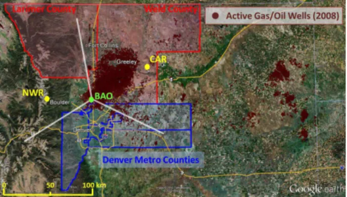
The BAO tower is located 25 km east-northeast of Boulder and 35 km north of Denver (40.05◦N, 105.01◦W). The base of the tower is at 1584 m above sea level (a.s.l.). As shown in Fig. 1, BAO is located at the southwestern edge of the DJB where a very large and dense network of oil and gas wells exists. Since late 2007 NOAA-GMD has been collecting dis-crete air samples approximately daily from 300 m. The air is collected in glass flasks and analyzed at NOAA-GMD for a suite of∼50 trace gases and then circulated to the Univer-sity of Colorado’s Institute of Arctic and Alpine Research (INSTAAR) for stable isotope measurements in CO2 and
CH4and preparation for14CO2measurement. The Center for
Accelerator Mass Spectrometry (CAMS) at Lawrence Liv-ermore National Laboratory (LLNL), which performed the
14CO
2measurements reported here, has participated in the
NOAA-GMD14CO2 discrete air sample measurement
pro-gram since 2009. This study focuses on data collected be-tween late June 2009 and September 2010, over which time 145 samples were analyzed for14CO2. More information on
this site and the entire tall tower network can be found at: http://www.esrl.noaa.gov/gmd/ccgg/towers/.
Standard meteorological measurements are also made continuously at several levels (10 m, 100 m, and 300 m, re-ported at 60 s, 60 s, and 30 s, respectively)) on the tower by the NOAA ESRL Physical Sciences Division (NOAA-PSD), including wind speed and direction, relative humidity, and temperature. We categorize each observation in our analysis according to wind direction (at 300 m) to facilitate a discus-sion of two distinct emisdiscus-sion source regions: the oil and gas industrial region to the north and east and the Denver metro region to the south. To do this, we define three wind sectors, consistent with those defined in the CFRPS: N/E (345◦ to 120◦), S (120◦to 240◦), and W (240◦to 345◦). These wind sectors are illustrated in Fig. 1. Wind sector boundaries are defined based on an analysis of the CH4/CO2ff ratio
variabil-ity with wind direction, which shows two distinct regimes for the CH4/CO2ff ratio (see Sect. 3.2). Wind direction for
Fig. 1. Map of northeast Colorado showing the BAO tower and the distribution of active oil and gas wells as of 2008 (updated well locations available at: http://cogcc.state.co.us/Home/gismain. cfm). Two background sites are also shown: Niwot Ridge (NWR; 3523 m a.s.l.) and the Briggsdale aircraft site (CAR). Also shown are the three wind sectors used to filter the dataset for emission esti-mates in Weld/Larimer counties (North and East) and in the Denver metro counties (South). The Denver metro counties include Denver, Broomfield, Adams, Arapahoe, and Jefferson. Top left corner of this map is: 41.064◦N, 106.248◦W.
a disproportionate influence from sources in the immediate vicinity of the tower. Using a filter of greater than 2.5 m s−1
leaves too few samples for a rigorous statistical analysis of the data. Supplementary Figs. S1 and S2 show the time series of mean wind direction and wind speed, respectively, associ-ated with each flask sample used in this analysis.
To define isotopic and mole fractions of trace gases in background air, measurements from two additional NOAA-GMD sites were used. For14CO2, CO2, CO, and CH4, we
used weekly measurements from Niwot Ridge, CO (sitecode NWR, 40.05o N, 105.63o W, 3526 m a.s.l.), a site in the alpine tundra with strong westerly winds that only rarely re-quired filtering of samples influenced by pollution from the Denver metro area (Turnbull et al., 2007). For other gases, in-cluding acetylene, benzene, and the C3–C5alkanes we used
weekly to fortnightly samples collected in the free tropo-sphere from flights at a nearby location (3000 to 4000 m a.s.l. above Briggsdale Colorado; sitecode CAR, 40.37o N,
104.30oW, ground elevation∼1700 m a.s.l.). 2.2 Flask sampling
Discrete whole air samples are collected daily (Andrews et al., 2013) from the BAO tall tower (from an air intake at 300 m) using Programmable Flask Packages (PFPs) con-nected to a Programmable Compressor Package (PCP) ca-pable of delivering 15 standard L min−1. Each PFP contains 12 cylindrical borosilicate glass flasks (0.7 L each). On each end of the flasks are automated glass-piston stopcocks, sealed with Teflon O-rings. Prior to deployment, each flask in the PFP unit is flushed with clean dry air and then pressurized to ∼140 kPa with synthetic air containing 330 ppm CO2.
Automated sampling consists of the following steps: (1) a manifold flush, (2) a flask flush, and (4) pressurization of the flask to∼270 kPa. The entire process takes about 2 min. Sampled air at BAO first passes through a drying stage (dew-point temperature at ambient pressure of∼5◦C) prior to col-lection. Sampling is done at midday (19:30 UTC) in most cases; all samples used in this analysis were collected within 30 min of 19:30 UTC. Two flasks are filled within 5 min of each other (∼4 standard liters) which provides enough air for analysis of the standard suite of trace gases (described below), and for analysis of14CO
2, which typically requires
0.4 to 0.5 mg C for high precision (<3 ‰) AMS analysis.
2.3 Flask analysis
Each flask pair is analyzed at NOAA–GMD for CO2, CO,
CH4, SF6, H2, N2O, and a suite of halocarbons and
hydro-carbons. Stable isotopes of CO2 (δ13C and δ18O) are
ana-lyzed at the INSTAAR Stable Isotope Laboratory (Vaughn et al., 2004). In this study, we use measurements of CO2, CO,
CH4, acetylene (C2H2), benzene (C6H6), propane (C3H8),
n-butane (n-C4H10), n-pentane (n-C5H12), and i-pentane
(i-C5H12). We also use δ13C in CO2 in the calculation of
114C, according to methods described by Stuiver and Polach (1977), which is required because the CAMS AMS does not measure the13C/12C ratio on-line.
Dry air mole fractions of CO2, CH4, and CO were
mea-sured on one of two nearly-identical custom automated ana-lytical systems. These systems consist of custom-made gas inlet systems, calibration systems, gas-specific analyzers, and system-control software. During this project, each sys-tem used a different technique to measure CO. One used a Reduction Gas Analyzer, where CO is separated from air by gas chromatography, then passed through a heated bed of HgO producing Hg before it is detected by resonance absorp-tion (Novelli et al., 1998). The second is Vacuum UV Reso-nance Fluorescence (VURF), where CO is detected by fluo-rescence at∼150 nm. Both techniques are calibrated against the same standard scale, and uncertainties (68 % confidence interval) are∼1 ppb for the VURF and∼2 ppb for the RGA. Long-term comparison of the two systems shows agreement to within∼1 ppb. CH4 was measured by gas
chromatogra-phy (GC) with flame ionization detection with an uncertainty of∼1.4 ppb (Dlugokencky et al., 1994). A non-dispersive in-frared analyzer is used for CO2with an uncertainty <0.1 ppm
(Conway et al., 1994).
The non-methane hydrocarbons (C2H2, benzene, and C3–
C5 alkanes) are measured using a gas
(3) uncertainty in assumed detector sensitivity due to ana-lyte losses during random and sporadic temperature anoma-lies during the pre-concentration step, and (4) chromato-graphic baseline interferences (propane only). Storage tests have shown negligible drift in the hydrocarbon mole frac-tions of reference gases. Therefore, assigned total uncertain-ties (1σ) are 5 % for n-C4H10, i-C5H12, n-C5H12, and C6H6,
and 15 % for C3H8due to chromatographic baseline
interfer-ences, and 15 % for C2H2due primarily to absolute
calibra-tion scale uncertainties. Measurement reproducibility (1σ) is generally <2 % for compounds present at mole fractions >10 ppt. For C2H2and C3H8, the most volatile of these
com-pounds, reproducibility was somewhat poorer during these flask analyses due to the instability of the temperature of the cryogenic pre-concentrator (approximately −25 % and +12 %). The asymmetric reproducibility is attributed to the different impact that the temperature instability has on quan-titation, depending on whether the anomalous temperature occurs during a BAO sample analysis or during analysis of the reference gas. This is primarily a problem only for the higher volatility species, C2H2 and C3H8. As this
temper-ature instability is a random, sporadic occurrence, we con-servatively allow for large negative uncertainties and smaller positive uncertainties in all analyses. An additional bias aris-ing from non-linearity in the GC-MS response to varyaris-ing an-alyte concentrations (except for propane, which is marginally linear) is estimated to result in an overestimate in the reported concentrations on the order of 5 % to 12 %. We do not include this bias implicitly in our emission calculations, but we dis-cuss its (minor) impact on our results and conclusions below. All measurements are reported as dry air mole fractions relative to internally consistent standard scales maintained at NOAA-GMD. We use the following abbreviations for mea-sured dry air mole fractions: ppm = µmol (trace gas) mol (dry air)−1, ppb = nmol mol−1, and ppt = pmol mol−1. Addi-tional details on these methods are described at http://www. esrl.noaa.gov/gmd/ccgg/aircraft/analysis.html.
2.4 Radiocarbon analysis
A subset (typically 1 out of every 2 pairs) of the flask pairs are hand selected for analysis of 14CO2. The
selec-tion is based on a visual inspecselec-tion of continuous CO and CO2 observations during the time of sampling. For a
typi-cal flask package, 3 pairs (out of the 6 pairs total) are se-lected for radiocarbon analysis, with two pairs typically hav-ing the highest CO and CO2 concentrations and one pair
having CO and CO2 concentrations closest to background.
This approach maximizes the dynamic range of the observa-tions over which tracer/CO2ff ratios are estimated. Analyses
of14CO2 were done by extracting CO2from the whole air
samples using cryogenic separation, reducing the extracted CO2 to graphite, and atom counting via accelerator mass
spectrometry (AMS). Extractions of authentic samples, mea-surement controls, and process blanks were performed at the
University of Colorado INSTAAR Laboratory for AMS Ra-diocarbon Preparation and Research (NSRL) using an auto-mated extraction system (Turnbull et al., 2010). Graphitiza-tion and AMS analysis was done at LLNL-CAMS. A de-scription of the high precision methods for analysis of atmo-spheric samples at CAMS is given by Graven et al. (2007). The measurements are expressed as age-corrected114CO2
in units of per mil (‰), calculated from the 14C/13C ratio (normalized to aδ13C of−25‰), measured relative to NBS Oxalic Acid I (OX1), and reported relative to the absolute ra-diocarbon standard, as detailed in Stuiver and Polach (1977). It should be noted that our use of114CO2, is equivalent to
the use of1in Stuiver and Polach.
Uncertainty in these observations is assigned as the stan-dard deviation (1σ) of a series of repeat measurements on extraction aliquots of whole air stored in high pressure cylin-ders. Air from two surveillance cylinders having different but near-ambient 14C activities, identified as NWT3 and NWT4, were extracted, graphitized, and analyzed concur-rent with the BAO samples across 7 diffeconcur-rent measurement “wheels” or batches. Multiple samples of NBS Oxalic Acid II (OX2, a commonly used secondary standard) were com-busted, graphitized and analyzed simultaneously. Typically, in a wheel containing 25 authentic samples, 12 measure-ment controls and 1 process blank were analyzed. For the observations described in this study, the (1σ) repeatabil-ity (standard deviation) of NWT3 and NWT4 samples was ±2.2‰ (n= 140). AMS measurement uncertainty (based on counting statistics) typically contributes about 1.3–1.7‰ of the total uncertainty. In a small number of cases, the inter-nal variability on the measurement of an unknown sample was larger than the repeatability of the pool of NWT sam-ples. The larger of the two is assigned as the uncertainty for a given114CO2measurement.
2.5 Calculation of CO2ff
Recently added fossil fuel CO2(CO2ff) is defined as the local
enhancement of CO2, with respect to an appropriate
back-ground reference site, due to fossil fuel emissions. CO2ff
is estimated using a mass balance approach (Levin et al., 2003), in which the observed mole fraction of CO2(CO2obs)
is partitioned into background CO2 (CO2bkg), fossil CO2,
and biogenic CO2(CO2bio) components. CO2bio is the net
balance between respired CO2 (CO2resp) and CO2 taken
up by photosynthesis (CO2photo). We further separate the
respired fraction into autotrophic respiration (CO2auto) and
heterotrophic respiration (CO2het) that originates from older
soil carbon pools (which typically contain more bomb14C). Equations (1a) and (1b) detail this mass balance relationship, as formulated in Turnbull et al. (2006), with CO2resp
observed114C.
CO2obs=CO2bkg+CO2ff+CO2bio (1a)
CO2bio=CO2auto+CO2het−CO2photo (1b)
114obsCO2obs=114bkgCO2bkg+114ffCO2ff+114bioCO2bio (2) Since114C values are all normalized by theirδ13C values, and thus are not influenced by natural fractionation, we can assume that114photoand114autoare identical to114bkg(Turnbull et al., 2006). The system of equations can then be solved for CO2ff to give Eq. (3).
CO2ff=
CO2obs(114obs−114bkg)
(114ff −114bkg) !
− CO2het
(114het−114bkg)
(114ff −114bkg) !
(3) In this equation, the variables in the first term are either known (114ff =−1000‰) or can be measured. We use ob-servations from NWR to estimate114bkg. The background is estimated by applying a smoothing algorithm (Thoning et al., 1989) to the NWR data (a curve-fit of 3 polynomials, 4 harmonics, and added low-pass filtered residuals), after fil-tering out samples influenced by upslope flows carrying lo-cally influenced air, characterized by high CO/CO2ratios, as
in Turnbull et al. (2007). Smoothed NWR results used here are from Lehman et al. (2013). The standard deviation of the residuals from the smoothing fit are calculated to be 1.7‰ . The selection of a proper background site is thought to in-troduce uncertainties on the order of the measurement tainty (∼2‰) (Turnbull et al., 2009). We define the uncer-tainty in CO2ff as 1.2 ppm, estimated from the measurement
uncertainty in114bkgand114obs(±2.2‰).
The second term in Eq. (3) is a minor correction to the cal-culation of CO2ff due to heterotrophic respiration from soils,
which can draw from carbon pools that are on the order of tens of years old, and thus reflect the higher114CO2in the
atmosphere at the time. The magnitude of this correction can be estimated from a terrestrial ecosystem model, such as the CASA biogeochemical model (Thompson and Randerson, 1999); we follow the estimates of Turnbull et al. (2009) for North American mid-latitudes and set this correction to−0.2 (±0.1) ppm (thus resulting in a positive offset) from October to March and to−0.5 (±0.3) ppm from April to September. Since the correction term in Eq. (3) is subtracted from the first term, the impact of heterotrophic respiration is to raise estimates of CO2ff in both seasons.
The influence of additional sources on 114obs is glob-ally variable and has potential contributions from strato-spheric intrusion of cosmogenically produced and bomb-era
14C (e.g. Levin et al., 2010; Graven et al., 2012a), nuclear
reactors (e.g. Graven and Gruber, 2011), biomass burning (e.g. Schuur et al., 2003; Vay et al., 2011), and the oceanic-atmosphere disequilibrium (e.g. Sweeney et al., 2007; Muller et al., 2008). However, model-based estimates of the114C signal (not including those from nuclear emissions) in the
conterminous United States (Miller et al., 2012) show that these terms contribute very little relative to the spatial gradi-ents arising from fossil fuel combustion. Graven and Gruber (2011) argue that in the eastern United States nuclear con-tributions may be significant, but they predict near-zero nu-clear influence in most of the western United States, includ-ing Colorado. Any contribution from stratosphere or ocean sources at BAO is likely to simultaneously impact the NWR background site and, thus, can be ignored in this analysis. At least one sample was influenced by a biomass burning event, identified by an anomalously high CO/CO2ff ratio, as well
as multiple news reports of poor air quality on that particu-lar day resulting from the Station Fire in southern Califor-nia in August 2009 (e.g. Brennan, 2009). This sample, along with one other that exhibits an abnormally high CO/CO2ff
ratio is omitted from this analysis. The sample influenced by the wildfire plume was collected 1 September 2009; the other sample, collected 30 January 2010, is unusual in that the estimated CO2bio mole fraction (calculated as CO2obs
– CO2ff–CO2bkg) was very large (15 ppm), and about twice
the estimated CO2ff for this sample. The large CO2bio
rela-tive to other samples in the dataset suggests the possibility of an undetected stratospheric or biomass burning influence or an unusually large heterotrophic respiration signal. We there-fore exclude this point (30 January 2010 sample) from our analysis. In addition to CO, a large number of other anthro-pogenic tracers were elevated in this particular sample, sug-gesting that stratospheric influence is, in the end, not likely.
2.6 Estimating tracer/CO2ff enhancement ratios
Tracer/CO2ff enhancement ratios are calculated by taking
the median of individual tracer/CO2ff ratios after
subtract-ing the background from each trace gas. The median ra-tios derived from individual samples provides a more ro-bust estimate of the apparent tracer/CO2ff ratios than that
determined from either a linear regression slope or an arith-metic mean, which may give estimates that are overly sen-sitive to ratio outliers that can result from signals due to air masses in which emissions of various sources are not well mixed (Miller et al., 2012). While the linear regression method has the advantage of being less sensitive to the se-lection of background site, when considering observations across seasonal to annual time scales a seasonally varying background may still bias the slope determination. Since the BAO tower and the NWR and CAR background sites are closely situated, it is likely that any background-related bi-ases are small. The tracer/CO2ff ratios are shown in Table 1.
For comparison, estimates of slopes are also provided in Ta-ble 1 for each tracer/CO2ff pair, derived using a two-way
Table 1.Summary of observed tracer/CO2ff ratios and associated uncertainties. Ratios estimated using the median point-by-point calculation
as well as from a two way linear regression. Correlation coefficients (r2) are also provided. For the C4and C5alkanes, C2H2, and benzene, a nonlinearity bias in the GC-MS response results in an estimated 5–12 % overestimate in the tracer/CO2ff ratios for these gases.
Species Wind Sector n Ratio (units) Ratio confidence n Slope (units) Slope confidence r2
limits (2σ) limits (2σ)
min max min max
CO N/E 43 8.8 (ppb ppm−1) 7.3 9.4 55 8.5 (ppb ppm−1) 7.1 10.5 0.70 S 22 10.5 (ppb ppm−1) 7.3 13.8 31 7.2 (ppb ppm−1) 5.7 9.6 0.89 Combined 65 9.0 (ppb ppm−1) 8.1 9.8 86 7.8 (ppb ppm−1) 6.5 9.3 0.83 CH4 N/E 43 31.3 (ppb ppm−1) 24.3 34.9 55 30.7 (ppb ppm−1) 22.1 34.5 0.81 S 23 9.5 (ppb ppm−1) 5.8 12.4 33 8.1 (ppb ppm−1) 5.0 11.4 0.75 C2H2 N/E 41 44.5 (ppt ppm−1) 39.8 52.5 53 63.6 (ppt ppm−1) 37.6 73.5 0.81 S 22 44.9 (ppt ppm−1) 34.7 61.6 32 45.2 (ppt ppm−1) 36.8 62.5 0.78 Combined 63 44.5 (ppt ppm−1) 40.7 51.8 85 52.1 (ppt ppm−1) 40.4 65.6 0.79 BENZ N/E 41 29.0 (ppt ppm−1) 22.2 36.5 53 33.7 (ppt ppm−1) 21.9 38.7 0.81 S 22 19.8 (ppt ppm−1) 14.8 26.2 32 14.2 (ppt ppm−1) 10.7 19.8 0.72 iC5H12 N/E 41 277.5 (ppt ppm−1) 243.1 395.9 53 485.2 (ppt ppm−1) 297.9 565.1 0.75 S 21 88.1 (ppt ppm−1) 47.6 120.7 31 65.4 (ppt ppm−1) 51.6 100.7 0.80 nC5H12 N/E 41 314.1 (ppt ppm−1) 236.8 402.4 53 480.6 (ppt ppm−1) 318.9 566.8 0.74 S 21 70.4 (ppt ppm−1) 37.4 106.0 31 54.5 (ppt ppm−1) 40.1 86.1 0.78 nC4H10 N/E 41 899.3 (ppt ppm−1) 707.9 1248.0 53 1520.8 (ppt ppm−1) 950.3 2085.1 0.71 S 21 193.3 (ppt ppm−1) 104.8 251.3 31 152.3 (ppt ppm−1) 102.6 212.8 0.75 C3H8 N/E 41 2035.2 (ppt ppm−1) 1615.8 2989.2 52 3265.1 (ppt ppm−1) 2048.4 4979.5 0.51 S 21 449.1 (ppt ppm−1) 243.3 612.1 31 352.7 (ppt ppm−1) 198.0 539.0 0.61
(r2). Samples are only used in the median ratio calculation when the estimated CO2ff is above the 1.2 ppm 1σdetection
limit to remove divide-by-zero errors, while no lower limit is used in the slope calculations. Removing this filter impacts the uncertainties of the median ratios (by up to∼50 %), but it has a smaller impact on the median ratios themselves, typ-ically impacting the tracer/CO2ff ratios by less than±10 %,
except for the C3–C5 alkanes in the S wind sector which
are impacted by between +15 and +30 %. In general, the application of this filter increases the enhancement ratios in the S wind sector and reduces them in the N/E wind sector. The supplementary material accompanying this manuscript includes figures (Figs. S3–S10) showing the data used to de-rive the median ratios, including time series and histograms of the dataset both with and without the wind speed and low CO2ff cut-off filters.
Uncertainties in the median ratios are 95 % confidence in-tervals, defined as the 2.5–97.5 percentile range (∼2σ con-fidence) from a distribution of 500 estimates of the median from a randomized re-sampling of the data (boot-strapping with replacement). We also estimated the uncertainty in the tracer/CO2ff enhancement ratios associated with
measure-ment uncertainty (both for the trace gas and CO2ff) and
found that these uncertainties (at 2σ) were comparable to or lower than the boot-strap approach in all cases. For C2H2,
n−C4H10,n−C5H12,i−C5H12, and C6H6, the nonlinearity
in the GC-MS response results, potentially, in an additional overestimate in the tracer/CO2ff ratios for these gases of as
much as 5–12 %. This bias has yet to be fully evaluated for
each gas, and is therefore not incorporated into the reported enhancement ratios.
A measure of the appropriateness of the tracer/CO2ff
ap-proach for deriving apparent emission ratios is estimated by calculating ther2 from a linear regression of tracers vs. CO2ff; a highr2 suggests that emissions of the tracers are
appreciably co-located with fossil fuel combustion sources. Results from the tracer/CO2ff enhancement ratio calculations
(with associated uncertainties, slopes, andr2values) are de-tailed in Table 1. Background observations for the different trace gases are taken from one of two nearby sites in the NOAA-GMD global network, either NWR (CO and CH4)
or from flights at CAR (acetylene, benzene, and the C3–C5
alkanes). CO and CH4observations are available from both
sites and we confirmed that the enhancement ratio estimates are not appreciably sensitive to the selection of background site (differences between 7 % and 15 % in derived enhance-ment ratios).
The sensitivity of this analysis to the prescribed het-erotrophic respiration correction to CO2ff (Eq. 3) was
deter-mined by recalculating the tracer/CO2ff ratios with this
cor-rection term doubled, in one case, and set to zero in another. The ratios estimated from this sensitivity test were within the 95 % confidence intervals in all but two cases (CO and C2H2), where the recalculated estimates were outside of the
confidence intervals only by a few percent. Thus, we consider the uncertainty in the heterotrophic respiration correction to CO2ff to be a largely insignificant source of error in our
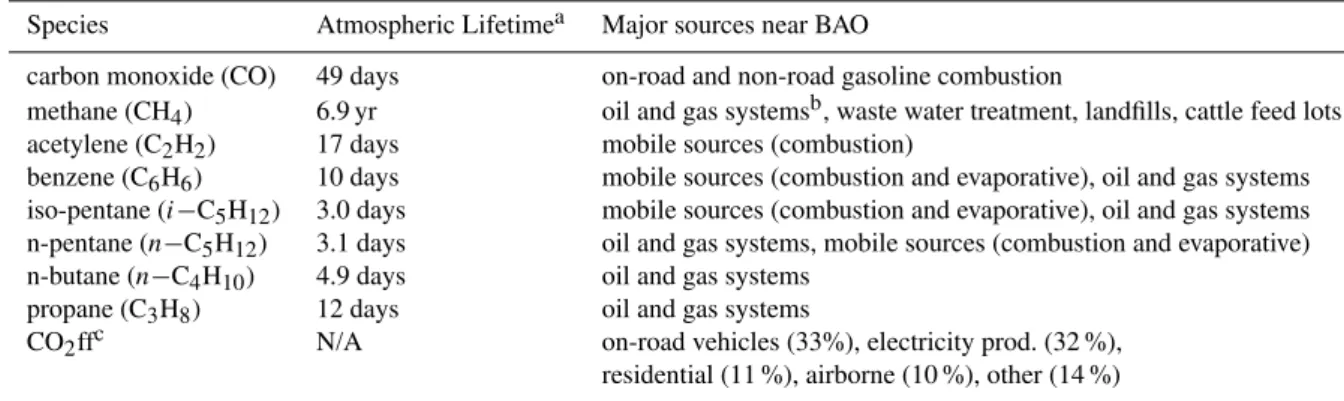
Table 2.Summary of trace gas lifetimes and major emission sources influencing observations at BAO (Watson et al., 2001; Pétron et al., 2012).
Species Atmospheric Lifetimea Major sources near BAO
carbon monoxide (CO) 49 days on-road and non-road gasoline combustion
methane (CH4) 6.9 yr oil and gas systemsb, waste water treatment, landfills, cattle feed lots
acetylene (C2H2) 17 days mobile sources (combustion)
benzene (C6H6) 10 days mobile sources (combustion and evaporative), oil and gas systems
iso-pentane (i−C5H12) 3.0 days mobile sources (combustion and evaporative), oil and gas systems
n-pentane (n−C5H12) 3.1 days oil and gas systems, mobile sources (combustion and evaporative)
n-butane (n−C4H10) 4.9 days oil and gas systems
propane (C3H8) 12 days oil and gas systems
CO2ffc N/A on-road vehicles (33%), electricity prod. (32 %),
residential (11 %), airborne (10 %), other (14 %)
aAtmospheric lifetimes estimated for [OH] = 1×106cm−3using published rate constant data (Atkinson et al., 2006; NASA, 2006).
bSources include condensate tanks, well drilling and completion, distribution systems, refineries.cSource distribution according to Vulcan v2.2 for Weld/Larimer and Denver metro counties in 2008.
surrounding BAO, it is more likely that the prescribed respi-ration correction is biased high rather than low, which would result in CO2ff values that are biased high and tracer/CO2ff
enhancement ratios that are biased low.
2.7 Bottom-up fossil fuel CO2emissions estimates
To derive top-down emissions estimates for the observed trace gases via tracer/CO2ff enhancement ratios, we use both
county-level and gridded bottom-up fossil fuel CO2
emis-sions estimates from the Vulcan data product (v2.2) (Gur-ney et al., 2009) as a quantitative reference. Vulcan (http: //vulcan.project.asu.edu) is a high resolution data product that utilizes a combination of energy, air quality, census, traf-fic, and digital road statistics to quantify fossil fuel CO2
emissions for the United States. Until recently, the Vulcan inventory was available only for 2002, but is now updated to include annual emissions at the county and state level for all years between 1999 and 2008. The gridded high resolu-tion product is currently available only for 2002, however. The Vulcan02 data product is used as the base year in this analysis. For the Vulcan02 product, country-wide emissions are in agreement with the United States Energy Information Administration (EIA) estimates to about 2 % even though the different estimates were compiled using independent statisti-cal datasets (Gurney et al., 2011). At the county level, the es-timated uncertainty (1σ) on annual CO2ff emissions from the
Vulcan02 data product is variable, but no more than∼20 % (and typically less than∼10 %) for any given county (Gurney et al., 2011). To apply the Vulcan02 data product to our anal-ysis period (2009–2010), the Vulcan02 emissions are scaled up to the observation period using the state-level EIA inven-tory (EIA, 2012), which is currently available through 2009. We use the county-level Vulcan data product for 2003–2008 to constrain the uncertainty in our scaling factor derived from the state-level EIA data. A more detailed description of the
scaling procedure and associated uncertainty is provided be-low (Sect. 3.3).
Vulcan emission rates for CO2are given in Table 3 for two
source regions that correspond to the N/E and S wind sec-tors, as defined above (Sect. 2.6). For simplicity we define the N/E wind sector as being influenced primarily by emis-sions from Weld and Larimer Counties and the S wind sec-tor as being influenced primarily by emissions from Adams, Broomfield, Arapahoe, Jefferson, and Denver Counties (col-lectively referred to here as the Denver metro counties). To-tal CO2ff emissions, according to Vulcan02, are estimated to
be 2.94 Tg C and 7.27 Tg C for the N/E (Weld and Larimer Counties) and S (Denver metro counties) wind sectors, re-spectively. The on-road, electrical production, residential, and airborne sectors contribute to 86 % of the total CO2ff
emissions in the region (Table 2). In Sect. 3.3.1, we consider the uncertainties associated with these assumptions about the geographic area influencing emissions in the two wind sec-tors.
2.8 Bottom-up trace gas emissions estimates
We compare our top-down emission estimates with bottom-up estimates for CO (NEI, 2008) and acetylene (NEI, 2005). Emissions of C2H2are estimated from a gridded NEI05
in-ventory of total VOC emissions in combination with the EPA SPECIATE(v4.3) model (EPA, 2011).
Table 3.Summary of top-down and bottom-up annual emissions for CO and C2H2, including the bottom-up emission source, inventory base
year, the scaling term (α), and associated uncertainties derived for different regions around the sampling site in Colorado for the measurement period. Bottom-up emissions for CO2ff are also summarized. Uncertainties on the scaled bottom-up emissions and the top-down emissions
are described in Sects. 3.3 and 3.3.1.
Species Wind Sector Bottom-Up Source Base α α Scaled Scaled Emissions Top-Down Ex Emissions Year (%) min/max Emissions Min/Max Emissions (Ex) Min/Max
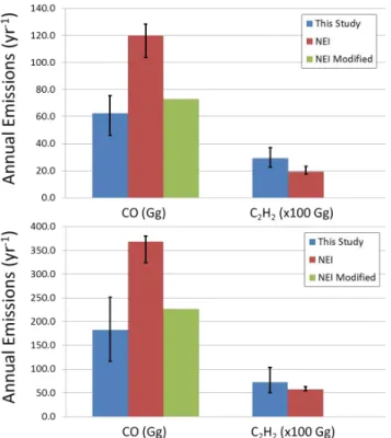
min max min max min max
CO N/E 116.0 Gg NEI08 2008 3.6 −10.5 11 120.1 Gg 103.8 128.4 62.4 Gg 46.0 75.5 S 362.1 Gg NEI08 2008 1.7 −10.5 5 368.2 Gg 324.1 380.5 182.5 Gg 116.8 251.2 Combined 478.1 Gg NEI08 2008 – – – 488.3 Gg 427.9 508.9 221.1 Gg 171.0 269.5 C2H2 N/E 0.172 Gg NEI05 2005 11.6 0 35 0.192 Gg 0.172 0.232 0.291 Gg 0.225 0.369 S 0.544 Gg NEI05 2005 5.2 0 16 0.572 Gg 0.544 0.629 0.727 Gg 0.506 1.034 Combined 0.643 Gg NEI05 2005 – – – 0.764 Gg 0.716 0.861 1.011 Gg 0.791 1.273
CO2 N/E 2.94 Tg C Vulcan2.2 2002 2.8 – – 3.02 Tg C 2.42 3.63 – – – –
S 7.27 Tg C Vulcan2.2 2002 2.8 – – 7.47 Tg C 5.98 8.97 – – – –
estimate using a scaling factor that is 3 times the popula-tion increase on the high end. An exceppopula-tion to this is for the uncertainty limits for CO emissions. There is evidence that on-road mobile CO emissions have decreased in many urban regions over the past 15–20 yr despite large population in-creases, and in Denver, specifically, the CO-to-fuel burnt ra-tio was observed to have decreased at a rate of about 7 % per year between 1999 and 2007 (Bishop and Stedman, 2008). Therefore, the bottom-up CO emissions uncertainty is brack-eted at the low end by an emission rate corresponding to a de-crease in emissions of 10.5 % from 2008 (the inventory base year) to the observation period. We acknowledge that scal-ing up of these trace gas estimates usscal-ing population statistics is an unconstrained approximation, and we have, therefore, assigned conservatively large uncertainties. It is important to note, however, that the inventory base year estimate is al-ways within the uncertainty brackets of the scaled inventory values, thus allowing the reader to evaluate the top-down and bottom-up comparison independent of any scaling assump-tions made here.
3 Results and discussion
3.1 114C and CO2ff time series
The results of the14CO2analyses are shown in Fig. 2a with
values ranging from−19.4 to 50.5‰. The time series runs from late June 2009 to September 2010, overlapping with the observation period of the CFRPS, where observations (from the same set of flask samples) up through the spring of 2010 were included in their top-down emission calcula-tions. Excursions of114CO2at BAO (relative to the NWR
background site) towards lower values signify the addition of recently emitted fossil fuel CO2to the sampled air mass.
As described in Sect. 2.5, the CO2ff mole fraction can be
quantified using Eq. (3), with an uncertainty of 1.2 ppm based on propagation of the analytical uncertainty in114CO2 for
both114obs and114bkg (the uncertainty in CO2terms is
Fig. 2.Time series of14CO2(a)and CO2ff(b)from 145 discrete
whole air samples (filled circles) collected at the BAO tower. Uncer-tainty in each14CO2measurement is±2.2‰, which translates to
an uncertainty in each CO2ff observation of 1.2 ppm (see Sect. 3.1). Thirty day binned medians are shown as open circles in both(a)and (b), with error bars representing the standard error of the mean (1σ) for each 30 day bin. Also shown in(a)is the14CO2background
as observed at NWR (black line) (Turnbull et al., 2007; Lehman et al.,2013), with the uncertainty envelope represented by the grey shaded region.
small relative to those for114C). Performing this calculation for each BAO observation in Fig. 2a gives CO2ff mole
frac-tions that range from below the 1.2 ppm detection limit up to 25 ppm. There are occasional instances of negative CO2ff
values (14 % of all samples), which is not physically real-istic. All but 5 of these samples (3 % of the entire dataset) lie within the 1σ envelope around zero and only 1 sample (−3.3 ppm) lies outside of 2σ, thus these negative values are statistically consistent with CO2ff = 0±1.2 ppm.
The most obvious feature of the CO2ff variability is that
relatively constant and lower, on average, during the summer months (Fig. 2b). This trend is qualitatively consistent with shallow, and variable, mixing layer heights in the winter and deep mixing layers in the summer (Turnbull et al., 2009). Mixing layer height is driven by a number of complex me-teorological and topographical variables, but largely by sur-face sensible heat flux, which is of course much lower dur-ing the winter. Tracer/tracer ratios are expected to be much less sensitive to variability in mixing layer height since the dilution and mixing of co-located and temporally co-varying emissions will impact the different tracers equally. As we de-scribe below, observations of a set of tracer/CO2ff ratios are
consistent with this expectation.
3.2 Variability in tracer/CO2ff enhancement ratios
When sources of trace gas emissions are co-located with fos-sil fuel combustion sources, an analysis of the trace gas en-hancements relative to CO2ff provides a means to better
un-derstand the variability in the mix of emission sources in-fluencing the site independent of the dilution and mixing dy-namics that impact absolute mole fractions. While variability in the absolute mole fractions of CO2ff has a strong seasonal
dependence (Fig. 2b), with larger enhancements observed in the winter than the summer, there is no apparent (statistically significant) seasonality to any of the considered tracer/CO2ff
enhancement ratios, suggesting that boundary layer dynam-ics are largely what are driving the seasonality in measured atmospheric mole fractions or that emissions of all the trace gases have similar seasonal cycles to CO2ff.
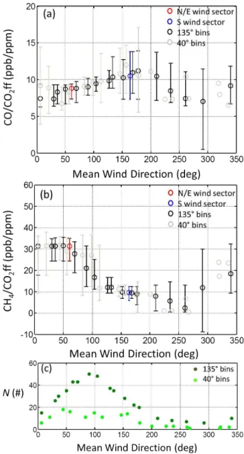
Figure 3a and b show the dependence of the CO/CO2ff
and CH4/CO2ff enhancement ratios on wind direction
us-ing two different size wind direction bins (40◦ and 135◦), demonstrating a significant enhancement in CH4abundance
(relative to CO2ff) when winds are arriving from the north
and east of the BAO tower. The CO/CO2ff ratio, on the other
hand, is relatively constant with wind direction such that the uncertainties in the different sectors overlap, suggest-ing a consistent mix of CO and CO2ff combustion sources
throughout the region. The CH4/CO2ff variability with wind
direction shows two distinct wind sectors within which the CH4/CO2ff ratio is relatively stable. A significant drop-off
in the CH4/CO2ff ratio can be seen at around ≥115–120◦,
which corresponds to sectors having fewer oil and gas wells and stronger influence from the Denver metropolitan region. This provides the basis for the definition of the N/E and S wind sector boundaries, which we use to examine differences in emissions for each trace gas considered in the analysis that follows.
The variability in CH4/CO2ff with wind direction is
con-sistent with results presented in the CFRPS (Pétron et al., 2012), which found significantly enhanced mole fractions of alkanes, including CH4, C3H8, n-C4H10,i−C5H12, and
n-C5H12, observed at BAO in air masses arriving from the N/E.
Benzene was also enhanced in air masses arriving from the
Fig. 3.Tracer/CO2ff ratios as a function of mean wind direction
for(a)CO and(b)CH4for each rotating 135◦-wide and 40◦-wide wind sector wedge. The number of observations in each 135◦and 40◦wedge is shown in(c). Also shown are the tracer/CO2ff ratios calculated for the N/E (red) and S (blue) wind sectors used in the analysis.
N/E. These differences were attributed to oil and gas produc-tion in Weld County, to the northeast of BAO. As shown on the map in Fig. 1, the majority of these wells are located in Weld County (COGCC, 2011), from which 17.9 million bar-rels of oil and 5.7 billion cubic meters of natural gas were produced in 2009 (COGCC, 2011). Other sources of CH4
subset of the gases considered: CO, C2H2, C6H6,i−C5H12,
and, to a lesser extent,n−C5H12(Watson et al., 2001). This
sector likely contributes significantly to emissions from the Denver metro counties, but there are also significant mobile emissions in the N/E wind sector from Interstate 25, the main north-south route in Colorado, as well as in a number of population centers, including Fort Collins, all located due north of BAO, in Larimer County. Table 2 summarizes the expected sources of the trace gases evaluated in this analysis, along with their expected atmospheric lifetime with respect to oxidation by OH. Lifetimes of the tracers considered range from 3 days (pentanes) to 7 yr (CH4) (calculated with a
con-stant OH density of 106cm−3). The oxidation of tracers can
potentially reduce the observed enhancement ratio, lowering the apparent emission ratio. However, with no statistically significant seasonal differences for any of the tracer/CO2ff
ratios, we see no evidence of strongly seasonal OH chem-istry impacting the tracer/CO2ff ratios discussed here. This
is likely a result of short transit times since emission relative to their atmospheric lifetimes.
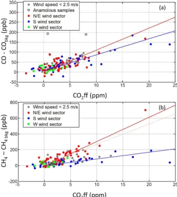
3.2.1 Carbon monoxide
Figure 4a shows the relationship between CO enhancement and CO2ff for each sample. Fits of a linear regression are
in-cluded in the Fig. 4a for the N/E and S wind sectors, giving
r2values of 0.70 (n= 55) and 0.89 (n= 31), respectively. As detailed in Table 1, the point-by-point analysis of these ob-servations show median (with 2σ equivalent confidence in-tervals) CO/CO2ff enhancement ratios of 8.8 (7.3–9.4) and
10.5 (7.3–13.8) for the N/E and S wind directions, respec-tively. For all wind sectors combined, the median ratio is 9.0 (8.1–9.8) (r2= 0.83).
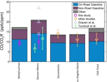
A comparison of these CO/CO2ff ratios with those found
in other studies and those predicted by bottom-up inven-tories are shown in Fig. 5. The observed ratios from both wind sectors are similar to the values of 6.8±2.2 and 11.7±5.5 ppb ppm−1 calculated at Niwot Ridge from two samples originating from the Boulder area via upslope winds in 2004 (Turnbull et al., 2006). Our estimates are somewhat lower, however, than previous reported values of CO/CO2ff
in Denver, where ratios were derived from linear correlations across 4 different aircraft flights (∼4-6 samples per flight) in May and July of 2004 (Graven et al., 2009). The observed ratios from these flights ranged from 14–27 ppb ppm−1.
Re-ductions in CO emissions from mobile sources between 2004 and 2009 are well documented (e.g. Bishop and Stedman, 2008) (part of a much longer term trend across most of the country), and could be a factor in the lower enhancement ra-tios observed here. The long term dataset from BAO, how-ever, provides a more robust estimate of the CO/CO2ff
ra-tio than either of these short-term studies where small er-rors in individual data points could result in a large differ-ence in the estimated ratio and where short term variabil-ity could have a strong influence. For comparison with these
Fig. 4.Correlation plots of CO(a)and CH4(b)enhancements (with
respect to background observations) with CO2ff. Data are
sepa-rated into three wind sectors (north and east: red; south: blue; and west: green), except in cases where average wind speeds were be-low 2.5 m s−1over the 30 min prior to sampling. Best-fit lines are shown for the N/E and S wind sectors (correlation coefficients are given in Table 1). In(a), two points are shown as open circles which are omitted from our analysis (see Sect. 2.5). In(b), a second best-fit line (light red) is shown for the N/E data, but excludes the highest CO2ff sample.
short term datasets, observed ratios of CO/CO2ff for
indi-vidual samples from the south wind sector at BAO range from 3.6 to 13.5 ppb ppm−1(1σ), with a maximum observed value of 20 ppb ppm−1(not including the sample impacted by biomass burning). Differences in the influencing area of emissions between the two studies may also play a role in the observed differences.
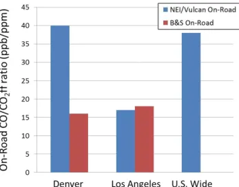
The main anthropogenic sources of CO in Colorado, and in much of the US, are from on-road gasoline vehicles in the mobile sector (66 %) and from non-road gasoline-based equipment (26 %) (NEI, 2008). While the on-road and non-road sectors account for 92 % of total CO emissions in Col-orado, these sectors contribute only 29 % of the total state CO2ff emissions according to the Vulcan08 data product
(Gurney et al., 2009). Therefore, the remaining 71 % of CO2ff sources contributes to at most 8 % of the total CO
NEI emissions estimate in Colorado. This suggests that the average CO/CO2ff emission ratio across a given region is
ex-pected to scale roughly with the fraction of CO2ff emissions
Fig. 5.A comparison of CO/CO2ff ratios observed or estimated in various US locations. The bars are calculated from bottom-up emis-sions estimates (NEI08 CO and Vulcan2.2 CO2) and color-coded
by the contribution of different sectors to the total CO emissions: on-road gasoline, non-road gasoline, and other. Observations from each location are shown, including those from our observations at BAO (split into Weld/Larimer and Denver metro influence based on wind sector) and observations from other studies: Denver (Turn-bull et al., 2006; Graven et al., 2009)), Sacramento (Turn(Turn-bull et al., 2011), LA Basin (which includes Los Angeles, Riverside, Orange, and San Bernardino counties) (Djuricin et al., 2010), and for the northeastern US (Miller et al., 2012).
Similar observed CO/CO2ff ratios for both N/E and S wind
sectors, therefore, suggests a similar contribution of on-road and non-road CO2ff sources in both Weld/Larimer counties
and the Denver metro counties, consistent with the Vulcan data product which estimates that the on-road plus non-road sectors (the dominant CO contributors) combine for 29 % and 41 % of the total CO2emissions, for Weld/Larimer and
Denver metro area respectively (Gurney et al., 2009). This is in contrast to CH4and other trace gases, as we discuss below,
where there is a clear enhancement due to non-combustion sources related to oil and gas production in the N/E sector.
3.2.2 Methane
We find significant differences in the mole fraction enhance-ment of CH4relative to CO2ff depending on wind direction
(Fig. 4b). The ratio in air arriving from the N/E sector is 31.3 (24.3–34.9) ppb ppm−1 and that for air traveling from
the S wind sector is 9.5 (5.8–12.4) ppb ppm−1. This higher
enhancement ratio in the N/E wind sector can also be vi-sualized in the correlation plot of CH4 enhancement with
CO2ff (Fig. 4b), where filtering by wind sector results in two
highly correlated relationships with different slopes. Anr2
of 0.81 (n= 55) and 0.75 (n= 33) is calculated for the N/E and S wind sectors, respectively. The high correlation in the N/E wind sector is influenced by the sample at relatively high
Fig. 6.Observed tracer/CO2ff ratios from Weld County (N/E wind
sector, red diamonds) and the Denver metro counties (S wind sector, blue circles). Ratios are calculated as the median of the point-by-point ratios for all data where CO2ff was detected above 1.2 ppm,
as described in Sect. 3.3. Uncertainties in the median ratios are the 95 % confidence intervals, defined as the 2.5–97.5 percentile range (∼2σconfidence) from a distribution of 500 median estimates from a randomized re-sampling of the data (boot-strapping with replace-ment). Note that the figure is presented using a logarithmic scale.
CO2ff (∼19 ppm CO2ff); removing this single data point
re-duces ther2to 0.65, but has little to no impact on the me-dian enhancement ratio (30.2 (22.6–34.9) ppb ppm−1). The median enhancement ratio is higher by a factor of 3 in the N/E wind sector relative to the S wind sector, implying that emissions of CH4, relative to CO2ff, are 3 times higher in the
N/E sector than the S sector. The added source of CH4
influ-encing air samples arriving from the N/E likely results from a mix of emissions from oil and gas operations in the DJB (Pétron et al., 2012), and other non oil and gas sources, such as cattle feedlots.
Entrained CO2ff can be co-emitted from natural gas wells,
but CO2 is only a small fraction (3–5 % by mass) of raw
natural gas (COGCC, 2011), and constitutes only a negli-gible fraction (< 0.1 %) of total Weld/Larimer county CO2
emissions, based on the CFRPS estimates. This suggests that while emissions of CH4 and CO2ff likely stem from
sepa-rate processes, there is sufficient co-location of sources such that air mass mixing prior to sampling has led to good corre-lations between these two gases in the BAO record. Further evidence of this can be found in a consideration of multiple tracer/CO2ff ratios, as discussed below.
3.2.3 Other trace gases
To further understand the differences in emission sources be-tween the two wind sectors, we consider the tracer/CO2ff
ratios for a number of additional gases. Figure 6 shows the difference in median tracer/CO2ff ratios for CO, C2H2,
CH4, C3–C5alkanes, and benzene when winds are from the
N/E and S sectors. Like CO, C2H2 is known to be
other gases are emitted either from non-combustion sources (C3H8, n−C4H10, and n−C5H12) or from a combination
of sources (C6H6 and i-C5H12). Both CO and C2H2
(rel-ative to CO2ff) show no appreciable dependence on wind
direction in our data, suggesting that both gases are emit-ted primarily from combustion processes that are common to Weld/Larimer counties and the Denver metro counties. The median ratio of C2H2 enhancement to CO2ff observed at
BAO (N/E and S combined) is 44.5 (40.7–51.8) ppt ppm−1 (16th–84th percentile range) (r2= 0.79, n= 85), which is consistent with observations from two previous studies in different US locations: 52 (45–59) ppt ppm−1downwind of
Sacramento, CA (Turnbull et al., 2011) and 45.9 (28.6– 102.9) ppt ppm−1off the east coast of the United States
dur-ing winter (Miller et al., 2012). This consistency suggests a relative insensitivity of this ratio to a particular mix of emis-sion type across the United States, an important criterion if one were to consider using C2H2as a proxy for CO2ff in the
absence of114CO2observations. However, the large spread
observed in the enhancement ratio off the eastern US coast by Miller et al. (2012) (as reflected by the 16th and 84th per-centiles of the distribution of observed ratios) suggests that there can be more variability in this ratio than indicated by the range of median values alone. Further, biomass burn-ing can be a significant source of C2H2, likely impacting
the C2H2/CO2ff ratio in different regions at different times
of year and from one year to the next. Additional research is required to better evaluate the potential for using C2H2
as a secondary CO2ff tracer and whether it would prove
ad-vantageous over the use of CO (Turnbull et al., 2006; Levin and Karstens, 2007), which may be problematic in locations where significant in situ CO production results from VOC oxidation.
As with CH4, there are significant differences in the
tracer/CO2ff enhancement ratios for the C3–C5alkanes and
benzene with wind direction, which suggests that enhanced emissions of these chemicals in the N/E are associated with gas and oil operations (Bar-Ilan et al., 2008a, b; Pétron et al., 2012). In general, ratios of C3–C5alkanes are enhanced
relative to CO2ff by about a factor of 4–5 in the N/E wind
sector compared to the S wind sector. Benzene is enhanced in the N/E wind sector compared to the S wind sector by a factor of 1.5. Despite the significant non-combustion sources of the VOCs related to gas and oil production, we see very good correlations of these species with CO2ff in air arriving
from the N/E (r2> 0.71, except for C3H8for whichr2= 0.51
and 0.61 for N/E and S, respectively) – an indication of in-tegration of emissions by air mass mixing or substantial co-location of combustion sources with oil and gas operations. The enhancement of the alkane/CO2ff ratios suggests, at least
qualitatively, that a significant portion of the CH4detected at
BAO stems from activities related to the oil and gas indus-try (Pétron et al., 2012), since agricultural emissions of CH4
are not expected to be associated with emissions of C3–C5
alkanes.
Fig. 7.Emissions estimates of CO and C2H2from Weld/Larimer counties (top) and the Denver metro counties (bottom). Top-down emissions, calculated using Eq. (4), are shown as blue bars, with uncertainties given as described in Sect. 3.3. Bottom-up emissions estimates from the NEI (2005 for C2H2and 2008 for CO)
inven-tory (red) are included for comparison for each species, as well as a modified bottom-up CO inventory as described in the text. Note the differences in units for the two trace gases.
3.3 Estimating emission magnitudes
From the observations described above as well as those re-ported in the CFRPS, it is clear that air sampled at the BAO tall tower is strongly influenced by emissions on local-to-regional scales (∼103-∼105km2). Changes in wind direc-tion at the site result in these local emissions coming from one of two primary source regions: (1) gas and oil operations to the north and east and (2) the Denver metro region to the south. Given the distinct geographical separation of sources, we use the wind sector specific observations, in conjunction with county-level CO2emissions from the Vulcan data
prod-uct (Gurney et al., 2009) as a means of estimating emissions for these trace gases using a tracer ratio approach.
Ex=ECO2ff(1+α /100) R (4) Equation (4) describes the annual average top-down emis-sions for a series of trace gases (Ex). For reasons described
below in Sect. 3.3.1, in this study we apply Eq. (4) to esti-mate emission magnitudes for CO and C2H2only. In Eq. (4),
interest, andαis a scaling factor that is designed to account for changes in emissions from the emission base year to the observation period. For CO2ff emissions, this factor is equal
to the change in emissions (expressed as a %) for the EIA inventory for Colorado between 2002 (the Vulcan base year) and the most current EIA inventory year, 2009. Equation (4) is applied independently to the N/E and S wind sectors for each tracer, withRcalculated for the N/E and S wind sectors paired withECO2ffestimates for Weld/Larimer counties and the metro Denver counties, respectively. Sinceαis based on state wide changes inECO2ff, this scaling factor is equivalent for both wind sectors. Tracer/CO2ff ratios (R) are calculated
as discussed in Sect. 3.2. Tables 1 and 3 summarize the pa-rameters used to calculateExfor Weld/Larimer counties and
the Denver metro counties. Note that after applying the wind direction, wind speed, and low CO2ff cut-off filters to the
dataset there are more accepted measurements in the dataset during winter than summer, and thus any seasonal bias in the observed valueRwould lead to winter emissions being over-represented in the estimates ofEx. From the available data,
however, we can detect no significant differences (with re-spect to the 2σconfidence intervals) inRwith season for the two gases considered. Additionally, we do not consider po-tential diurnal or day-of-week variability in emissions in this analysis. Since all the samples were collected at the same time of day – within 30 min of 12:30 local time, the derived emissions and emission ratios will be biased towards daytime (vs. nighttime) emissions. Weekends are slightly over sam-pled in this dataset (2.5 weekend samples for every 7 total samples) which could lead to a slight bias towards weekends in the annual emissions estimates; however, we do not find any statistically significant weekday-to-weekend differences in the tracer/CO2ff ratios.
Uncertainties inR(as described in Sect. 3.2),ECO2ff, and
α are considered in the estimation of top-down emissions. The scaling term,α, is 2.8 % for the state of Colorado ac-cording to the EIA inventory. While this scaling term indi-cates almost no change between 2002 and 2009 emissions, in actuality, EIA emissions increased by 9 % by 2007 and then decreased over the next 2 yr (presumably related to the economic downturn in the United States during this pe-riod). Similar trends are observed in the county level Vul-can emissions over this time period, though the peak year in both Denver Metro and Weld/Larimer counties occurs earlier than 2007. Using changes in the annual EIA-based Colorado emissions to scale the Denver Metro and Weld/Larimer Vul-can02 estimates, gives, in general, very good agreement with the Vulcan estimates for these counties from 2003–2008 (to within 10 % for any given year and about 5 % on average). The Vulcan02 uncertainties (1σ) for the annual emission es-timates from individual counties considered here are of sim-ilar order, ranging from 4.6 % to 10.6 %, (K. Gurney, unpub-lished results) with less uncertainty associated with the com-bined larger county “sectors” that we use in our wind sector analysis. Doubling these uncertainties (to be consistent with
our 2σ analysis) for the two wind sectors results in differ-ences from the central estimate of 7 % (upper estimate) and 11 % (lower estimate) for Weld/Larimer counties and 7 % (upper) and 10 % (lower) for the Denver metro counties. We therefore assign a conservative uncertainty of±20 % to the scaled bottom-up CO2ff emissions estimates in this analysis,
in which includes both uncertainty in bothECO2ffandα. It should be noted that the Vulcan estimates may include emissions of modern (non-fossil) CO2from the on-road
sec-tor in locations where biofuels (ethanol) are used, including Colorado, which would lead to a positive bias inECO2ff, and therefore,Ex. This bias would scale directly with the
frac-tion of total CO2ff (all sectors) in the Vulcan estimate that
is from biofuels. For some perspective, a fleet-wide 15 % biofuel blend in the on-road sector (33 % of the total CO2ff
emissions in the region; see Table 2) would result in a+5 % bias in our estimates ofEx, which we consider small
com-pared to other uncertainties. This would be roughly equiva-lent to assigning a value of−950‰ (rather than -1000‰) for
114ff in our derived CO2ff estimate.
The calculated top-down emission magnitude estimates (Ex) are given as a central estimate or ‘best guess’ for the
an-nual emissions plus 95 % confidence intervals calculated by propagation of the uncertainties described above. The boot-strap determination of uncertainties for the enhancement ra-tio provides a reasonable approximara-tion of the impact of the variability of the tracer/CO2ff ratios. Figure 7 summarizes
the top-down estimates and confidence intervals (whiskers), along with the available bottom-up estimates, for CO and C2H2for each wind sector.
3.3.1 Spatial considerations
Additional uncertainty inECO2ff arises as a result of our as-sumptions regarding the geographic footprint (area of emis-sions) influencing the observations. Obviously, the emissions influencing the observations are not strictly confined to the county boundaries that we have selected, based on the simple wind sector analysis. This matters only to the extent that the spatial distribution of tracer/CO2ff emission ratios varies
be-tween the presumed footprint and the actual footprint. This may be an issue especially for emissions estimates in the N/E wind sector where we expect VOC and CH4emissions
from the DJB to be primarily confined to within Weld County while CO2emissions are likely significant over a larger
spa-tial scale. For example, there are significant CO2emissions
along the I-25 corridor (in Larimer County) to the north of BAO, where there are relatively few active gas wells (see Fig. 1). Further, whereas CO2ff emissions are significant in