Adv. Sci. Res., 4, 77–82, 2010 www.adv-sci-res.net/4/77/2010/ doi:10.5194/asr-4-77-2010
©Author(s) 2010. CC Attribution 3.0 License.
Advances
in
Science & Research
Open Access ProceedingsEMS
Ann
ual
Meeting
and
9th
European
Conf
erence
on
Applications
of
Meteorology
2009
Tornado-type stationary vortex with nonlinear term
due to moisture transport
P. B. Rutkevich1and P. P. Rutkevych2
1Space Research Institute (IKI), RAS, Moscow, Russia
2Institute of High Performance Computing, A*STAR, Singapore
Received: 24 December 2009 – Revised: 11 May 2010 – Accepted: 14 May 2010 – Published: 14 June 2010
Abstract. Tornado vortex is believed to be essentially nonlinear phenomenon; and the puzzle to choose the nonlinear term(s) responsible for its formation is still unresolved. In the present work we consider the non-linear term associated with atmosphere humidity, by introducing variable temperature gradient depending on the vertical velocity of the fluid. Such term is able to yield energy to the system and is very suitable for such a problem. Other nonlinear terms are neglected, assuming slow rotation, or in other words a “weak” tornado approximation. We consider one-dimensional radial boundary problem, and use a modificaiton of shooting
method to satisfy boundary conditions at large radii. Obtained numerical solutions of the nonlinear differential
equation qualitatively agree with the observed atmosphere vortices (tornados, tropical cyclones). The obtained results show general possibility of existence of unstable motion even in convectively stable atmosphere strati-fication.
1 Introduction
Formation mechanisms and internal structure of severe at-mospheric vortices have been important questions over the past decades. In spite of their importance for both theory and applications, there is no satisfactory theory of tornado struc-tures (Doswell and Burgess, 1993) and recently there is a tendency towards collection of observational data or numer-ical simulation of the phenomenon (Bluestein et al., 1997; Bluestein and Pazmany, 2000; Bluestein and Weisman, 2000; Lehmiller et al., 2001).
The problem of tornado formation appears to be com-plicated from both principal and technical points of view. Tornado descends from a long-living rotating thunderstorm cloud. Having appeared from the cloud the funnel narrows in its upper part and dynamically stretches in the bottom part, however the middle part of the tornado column remains cylindrical and almost unchanged during the entire lifetime of the funnel. Such structure is especially pronounced for weak tornadoes (Davies-Jones, 2001), i.e. for tornadoes with high ratio of the height to the diameter. Mathematical model of the middle part of tornado should have a steady-state so-lution or soso-lution with very low growth rates.
Correspondence to:P. B. Rutkevich (peter [email protected])
It is commonly accepted that tornado solution cannot be derived from linear system of equations (continuity, Navier-Stokes, entropy) and therefore it is believed that tornado is described by a set of nonlinear hydrodynamic equations. However, it is still unclear which non-linear processes are responsible for its formation. Indeed, the inertia non-linear
terms (v∇)vlead to energy dissipation, therefore cannot be
the energy source of the system. Other non-linear terms have the same problem, since they do not introduce energy in the system.
Renno and Ingersoll (1996) described convection in the atmosphere as a heat engine between warm surface (due to solar radiation) and cold troposhpere, this assumption im-plies heat accumulation and release by means of black-body radiation. However, continuous and powerful source of en-ergy observed in tornadoes and cyclones has to come from
a source much more efficient than the black body radiation
or heat conductivity. One of possibilities is to use latent heat of water vapor as the source, since vapor content in the air is widely spread in the atmosphere, phase transitions occur fast, and the specific condensation energy is high. In this work we imply a mechanism of the latent heat release by
varying the vertical temperature profiles in different parts of
the tornado structure. Unlike a heat engine, the process is
not reversible. Indeed, at different points the tornado has
troposphere, respectively. The upwards fluid flow transports the vapor, which constantly condenses and releases the heat at all levels. Therefore the vertical temperature profiles in
these two flows are essentially different. As it will be shown
later, such system has a stable configuration with strong ver-tical and azimuthal velocity components.
2 Formulation of the problem
We start from the full system of hydrodynamic equations for compressible fluid, consisting of continuity equation, Navier-Stokes equations, and entropy balance (Landau and Lifshitz, 1987):
∂ρ
∂t+∇(ρv)=0, (1)
∂v ∂t−ν∇
2
v+(v·∇)v=−∇ P
ρ +2Ωez×v+ezg, (2) ∂s
∂t+(v·∇)s=
χcP
T ∇
2T,
(3)
where thermal diffusivity coefficientχ=k/(cPρ) is used
in-stead of the thermal conductivityk, andcP is specific heat
capacity of air at constant pressure; ν is the kinematic
tur-bulent viscosity, ezΩis the vector of angular velocity of the
rotating mothercloud, andvis the fluid velocity. Although
we describe compressible fluid, we have neglected in Eq. (2) the term with bulk viscosity for simplicity.
We introduce cylindrical coordinates with unit vector
ez directed upward. Following the standard linearization
procedure (Landau and Lifshitz, 1987), density, pressure
and temperature are represented as ρ(r,z)=ρ0(z)+ρ1(r,z),
P(r,z)=P0(z)+P1(r,z) and T(r,z)=T0(z)+T1(r,z),
respec-tively. Here the steady-state adiabatic profiles of thermody-namic functions are denoted by index 0, and their small per-turbations by index 1. The linearization procedure requires perturbations to be small compared to the steady-state values i.e. “weak” tornado.
The steady-state profiles are determined in an assump-tion of zero velocities, implying the temperature profiles are close to adiabatic. The corresponding set of equations
con-tain steady-state Navier-Stokes equations ∇P0+ezgρ0=0,
the perfect gas lawP0=ρ0RT0, and the steady-state entropy
balance equation:∇2T
0=0. Solution of the latter equation is
a linear temperature profile, which we postulate as
T0(z)=T00+γz=T00+(γa+γ′)z, (4)
where T00=T0(0) is the temperature value near the
sur-face, γa=−g/cP is a well known neutral adiabatic
gradi-ent of dry atmosphere, and γ′ is the deviation of the
cho-sen steady-state gradient γ from the neutral profile γa,
g is the gravity acceleration. According to our
steady-state assumption the deviation is small: γ′≪γa, and
pos-itive value of γ′ corresponds to convectively stable
atmo-sphere. Substituting temperature profile (Eq. 4) into steady-state Navier-Stokes equations one can derive the pressure
P0(z)=P00[T0(z)/T00]−g/(Rγ)≈P00[T0(z)/T00]κ/(κ−1), and
den-sityρ0(z)=ρ00[T0(z)/T00]−g/(Rγ)−1≈ρ00[T0(z)/T00]1/(κ−1),
pro-files whereκ=cP/cVis the ratio of specific heats. Notice the
density derivative
1 ρ0
∂ρ0 ∂z =−
g
c2, (5)
wherec(z)=√κRT0(z) is the sound velocity.
Linearization with the steady state Eqs. (4)–(5) leads to the following linearized system of hydrodynamic equations:
∂ρ1 ∂t +vz
∂ρ0
∂z +ρ0∇ ·v=0, (6)
∂v ∂t−ν∇
2 v+∇
P1 ρ0
+gezρ1
ρ0
+2Ωez×v=0, (7)
∂P1 ∂t −c
2∂ρ1 ∂t +κRρ0γ
′
vz=χκ∇2P1−c2χ∇2ρ1−2Rκχγa ∂ ∂z
ρ1 ρ0
. (8)
To derive the last equation we have used the perfect gas
entropy ass=cPln(T/T00)−Rln(P/P00), substituted here the
pressure and temperature profiles, expressed the temperature through the pressure and density using the perfect gas law, and finally substituted this entropy into Eq. (3).
Now we are constructing a steady-state (∂/∂t=0), isotropic
(∂/∂θ=0), and vertically homogeneous (∂/∂z=0) solution of
the linearized system (Eqs. 6–8). It is convenient to express velocity in terms of potential, toroidal, and poloidal fields (Rutkevich and Rutkevych, 2009):
v=∇Φ +∇ ×(ezψ)+∇ ×(∇ ×(ezϕ)), (9)
whereΦ(t,r),ψ(t,r) andϕ(t,r) are the potentials of the above
mentioned velocity components. In terms of these variables the set of Eqs. (6)–(8) becomes
∆Φ +g
c2∆ϕ=0, (10)
−ν∆∆Φ +∆P1
ρ0 +
g2
c2 ρ1
ρ0+2Ω∆ψ=0, (11)
−ν∆∆ψ−2Ω∆Φ =0, (12)
−ν∆∆∆ϕ+ g
c2
∆P1
ρ0 −
g
ρ0∆ρ1=0, (13)
−κRγ′(vz)ρ0∆ϕ−χκ∆P1+χc2∆ρ1=0, (14)
where ∆ =∇2r = 1r
∂ ∂r
r∂r∂ is the radial component of the
Laplace operator. The system of ordinary differential
Eqs. (10)–(14) describes the radial profiles of the
thermo-dynamic parameters and velocities at any given heightz=z0,
i.e. at given densityρ0(z0) and sound velocityc(z0).
the temperature profile on the vertical velocity of the fluid. In this work we use a simple approximation
γ′(vz)=γ0+γ1v z
vT
, (15)
whereγ0>0 is the temperature gradient of stable dry
atmo-sphere, coefficientγ1<0 accounts for the temperature profile
in moist air, andvTis the velocity normalization coefficient.
For sufficiently high vertical velocityvzthe total temperature
gradient (Eq. 15) becomes negative (i.e. convectively unsta-ble).
3 Convection without rotation
In non-rotational (Ω→0) and incompressible (c→∞) fluid
the system Eqs. (10)–(14) reduces to one equation for the
poloidal velocity potentialϕ:
∆2ϕ+ gγ
′
T0(z0)νχ
ϕ=0. (16)
Other velocity components, pressure and density can be de-rived from the solution of Eq. (16). Now we substitute the
temperature gradient (Eq. 15) in Eq. (16), expressvzin terms
ofϕby means of Eq. (9), and obtain the following nonlinear
equation
∆2ϕ+ gγ0
T0(z0)νχ ϕ−γ1
γ0 ϕ∆ϕ
vT
!
=0, (17)
or in dimensionless variables
∆2xf+f−f∆xf=0, (18)
wherer=λxandϕ=C f, and
λ= T0(z0)χν
gγ0 !1/4
, C=γ0
γ1λ 2
vT, ∆x=
1
x
∂ ∂xx
∂
∂x. (19)
Note, that according to this definition the coefficientCis
neg-ative. The unknown function f(x) has to be a regular
func-tion of its argument, therefore solufunc-tion of Eq. (18) can be
expanded in a Taylor series nearx=0:
f(x,A,a2)=A
1+a2x2+
∞
X
j=2
a2jx2j
, (20)
where only two coefficients are independent. Indeed, one can
easily check that coefficientsa4,a6, etc, can be recursively
expressed in terms of parameters Aanda2 using Eq. (18).
Construction of the solution (Eq. 20) for largexis
computa-tionally intensive due to fast divergence of the series, there-fore we use 4-th order Runge-Kutta method to build a numer-ical solution of Cauchy problem for the 4-th order ordinary
Eq. (18), using the values of function f(x) and its
deriva-tives at pointx=0.1, as calculated from the Taylor expansion
(Eq. 20). It appears impossible to apply Runge-Kutta method
fromx=0 due to singularity of the Eq. (18).
3.36
3.364
3.368
3.372 -0.2661 -0.2657
-0.2653 -0.2649 10
15 20 25
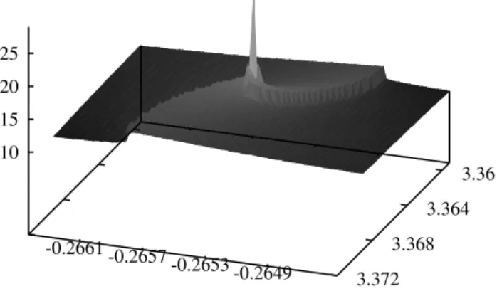
Figure 1. Profile of thexmversus the parametersa2 andA. The peak position indicates the best approximation of the solution of the nonlinear Eq. (18) in non-rotational fluid.
For arbitrary values of parameters A and a2 solution
(Eq. 20) diverges even for moderate x. However, the
lo-calized solution of our interest here should have a non-zero value near the axis, gradually vanish at medium distance from the axis, and uncontrollably grow far away from the
axis due to numerical errors. We denotexm(A,a2) the
maxi-mum value of dimensionless radius in the far-away rangex>
10, where the solution is small enough |f(xm,A,a2)|<b|A|.
Herebis a fixed number in the range 0<b<1, and the
“far-away” radiusx=10 corresponds tor=700 m, which we
sup-pose sufficiently large. Let us denoteA0anda2,0the values of
parametersAanda2, corresponding to the solution (Eq. 20)
vanishing atx→ ∞. It is clear that functionxm(A,a2) defined
above should go to+∞, asA→A0,a2→a2,0.
Equation (18) has to be solved numerically, therefore the
exact values (A0,a2,0) are hardly obtainable, however, one
can approximate the solution by choosing parameters (A,a2),
which give large enough value for the function xm(A,a2).
In this case the best solution would be the solution with
the biggest value of xm. In our numerical scheme the
co-efficientsA anda2 were varied simultaneously (see Fig. 1)
to obtain maximum value of xm(A,a2). The sharp peak on
the plot corresponds to the best approximation of solution
f(x,A0,a2,0) of the nonlinear equation (18). The position
of the peak is at A≈ −3.3641719 anda2≈ −0.265424,
giv-ing the maximum dimensionless radiusxm≈25. The
corre-sponding solution of dimensionless poloidal potentialf(x) is
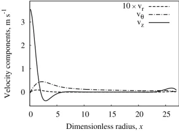
shown in Fig. 2. Corresponding velocity profiles (vr,vθ,vz)
are plotted in Fig. 3 for the following values of parameters:
g=9.8 ms−2,ν=χ=30 m2s−1,γ0=10−3km−1,γ1=−10−3
km−1,
vT=1 ms−1,κ=1.4,T0=280 K,c=335 ms−1.
It should be noted here, that strictly speaking the radial
and azimuthal velocity components (vr andvθ) are not
-4 -3 -2 -1 0
0 5 10 15 20 25
Poloidal velocity potential
f(x)
Dimensionless radius, x
f(x)
Figure 2. The best approximation of dimensionless poloidal ve-locity profile f(x). The values of the parametersAand a2 in the Taylor expansion (Eq. 20) correspond to the position of the peak in Fig. 1.
velocity components from the known profile of f(x), using
definition (Eq. 9) and system (Eqs. 10–14) as:
v=er g|C|
c2λ ∂f
∂x−eθ
2Ωgλ|C|
νc2x
x
Z
0
x′f(x′)dx′+ez| C|
λ2∆xf. (21) Azimuthal component of the velocity is proportional to the
rotation speed of the mothercloud. The profile ofvθin Fig. 3
has been plotted for Ω =0.1 s−1. For the chosen values of
parameters the radial and azimuthal components are signifi-cantly smaller than the radial component. This fact is in ac-cordance with the initial assumption of non-rotational fluid
(Ω→0). Noteworthy, that the radial velocity of the fluidvris
positive near the axis, indicating continuous expansion of the gas during its upwards movement.
Another noteworthy conclusion is that the dimensional
pa-rameter λdecreases with decreasing temperature (Eq. 19).
This means that for other constant conditions the radius of the tornado column decreases with hight. However, this
ef-fect is of the order of 1–2% for temperature variation of±5%
(i.e. tornado height below 2 km).
4 Convection with rotation
Taking into account compressibility of the gas (i.e.c,∞) and
its rotation (Ω,0), one can reduce the linearized system (10)–
(14) to a single high-order ordinary differential equation for
the poloidal field ϕ. Again we assume vertically
homoge-neous (∂/∂z=0), isotropic (∂/∂θ=0), and stationary (∂/∂t=0)
system. Using the same dimensionless units (Eq. 19) the equation reads as
∆x∆x∆xf(x)+f(x)−f(x)∆xf(x)−Q f(x)=0, (22)
0 1 2 3
0 5 10 15 20 25
Velocity components, m s
-1
Dimensionless radius, x
10 × vr vθ vz
Figure 3. Profiles of velocity components in a non-rotational ap-proximation. Values of parameters are listed at the end of Sect. 3. Notice a factor in front of the radial velocity componentvr.
where dimensionless parameter Q=(κ−1)(2Ωgλ3)2ν−2c−4
characterizes the Coriolis force and compressibility. Clearly,
in the caseQ=0 one obtains Eq. (18).
Due to 6-th order of Eq. (22), the expansion coefficientsa6,
a8etc. can be derived from givenA,a2,a4, therefore the
solu-tions now form a three-parameters set f(x;A,a2,a4), making
the numerical search procedure significantly more compli-cated. To solve Eq. (22) we apply the procedure described in Sect. 3, including Taylor series expansion in the vicinity of
x=0 and Runge-Kutta numerical solution from x=0.1. Due
to higher noise in the function, the values of the three inde-pendent parameters have been varied to achieve the smallest
possible value of integral Rxx2
1 f(x)
2dx
, instead of the
max-imumxmdescribed earlier. This choice of the convergency
condition reflects the fact, that the absolute value of the
func-tion f should be the smallest in the medium range of radii.
Figure 4 shows the best numerical solution, which we have
found in such a way, usingx1=8, x2=14, and givenQ=0.1.
The solution corresponds to the following set of parameters:
A≈11.29547,a2≈ −5.454639,a4≈ −2.179057. One can see,
that the found solution diverges atxm≈13.
The radial and vertical velocity components can be
ob-tained from the potential profile f(x) using Eq. (21), while
for the azimuthal profile one has to solve differential
equa-tion
∂vθ(r)
∂r + vθ(r)
r +
2Ωg
νc2 ϕ(r)=0. (23) Velocity profiles are plotted in Fig. 5. The air motion has several important features, namely updrift in the central area, relatively small radial velocity, and azimuthal velocity has
maximum at approximatelyx≈8. The azimuthal velocity in
-125 -100 -75 -50 -25 0 25 50
0 4 8 12
Poloidal velocity potential
f(x)
Dimensionless radius, x
f(x)
Figure 4.Profile of dimensionless potential fieldf(x) with rotation. The values of parameters are the same as the non-rotational case, except the Coriolis parameterΩ=0.23 s−1.
-200 -100 0 100 200 300
0 4 8 12
Velocity components, m s
-1
Dimensionless radius, x
100 × vr vθ vz
Figure 5.Profiles of velocity components with rotation, parameter values are the same as in Fig. 4.
of the fluid. In our simulation the azimuthal velocity changes the sign and infinitely increases, however we suppose this is an artifact of the numerical method. The expected
conver-gency region of the azimuthal velocity is in the rangex≥x2,
where the profile f(x) used in Eq. (23) has large errors. The
actual profile of azimuthal velocity, which can be regarded as fine-tuning of the solution, is a subject of further study.
The coefficient λ used for dimensionless radii (Eq. 19)
equals to 70 m for the chosen values of parameters. There-fore one can conclude, that the main upward air stream in Fig. 3 has radius slightly more than 100 m. Although this value is relatively large for a tornado, the model does not in-clude the rotation, which is likely to sharpen the structure. Indeed, solution with rotation in Fig. 5 has the radius of the upwards flow less than 70 m, which is very close to a typical tornado size (Davies-Jones, 2001).
The absolute value of velocity of 3 ms−1in non-rotational
case is reasonable, since effectively this is the velocity of a
free localized convection in atmosphere. Account of rotation in the system leads to dramatic growth of velocity, especially its vertical component. This suggests that a model of tornado must include other non-linear dissipating terms to suppress the fluid flow.
5 Conclusions
The proposed one-dimensional vertically-homogeneous model cannot be applied to the tornado funnel near the moth-ercloud, or to the turbulent area near the ground surface. The model is applicable at the middle level of a weak tornado, where the shape of the column changes slowly in space and time. The model shows that the system of linearized hydro-dynamic equations can have a stable solution with only one non-linear term. Since the full system of equations has sev-eral important non-linear terms (including viscosity and cen-trifugal force) this paper cannot be regarded as the final solu-tion of the hydrodynamic system or as a complete theory of tornado. However, the results show, that a steady-state con-figuration is possible even in convectively-stable atmosphere.
Proposed non-linear effect related to asymmetric vapor
transport in a “weak” tornado-like structure introduces the source of energy, which can be the true mechanism in natural
intensive vortices. Obtained structures have all features
of real tornadoes/cyclones, however estimations show that
the size of the solution is closer to the size of tornado. We expect, that accounting other non-linear terms (which are usually dissipating) in the full system of equations will lead to stabilization of the solution and especially far from the axis.
Edited by: D. Giaiotti
Reviewed by: two anonymous referees
References
Bluestein, H. B., Gaddy, S. G., DowelL, D. C., Pazmany, A. L., Galloway, J. C., McIntosh, R. E., and Stein, H.: Doppler Radar Observations of Substorm-Scale Vortices in a Supercell, Mon. Weather Rev., 125, 1046–1059, 1997.
Bluestein, H. B. and Pazmany, A. L.: Observations of Tornadoes and Other Convective Phenomena with a Mobile, 3-mm Wave-length, Doppler Radar: The Spring 1999 Field Experiment, B. Am. Meteorol. Soc., 81, 2939–2952, 2000.
Bluestein, H. B. and Weisman, M. L.: The Interaction of Numeri-cally Simulated Supercells Initiated along Lines, Mon. Weather Rev., 128, 3128–3149, 2000.
Davies-Jones, R.: Severe convective storm, Vol. 28, Meteorological Monographs, 2001.
Church, C., Burgess, D., Doswell, C., Davies-Jones, R., Geo-phys. Monogr, Vol. 79, Amer. GeoGeo-phys. Union, 161–172, 1993. Landau, L. D. and Lifshitz, E. M.: Fluid Mechanics, 2nd Edn.,
1987.
Lehmiller, G. S., Bluestein, H. B., Neiman, P. J., Ralph, F. M., and Feltz, W. F.: Wind Structure in a Supercell Thunderstorm as Measured by a UHF Wind Profiler, Mon. Weather Rev., 129, 1968–1986, 2001.
Renno, N. O. and Ingersoll, A. P.: Natural convection as a heat engine: a theory for CAPE, J. Atmos. Sci., 53, 572–585, 1996. Rutkevich, P. B. and Rutkevych, P. P.: Model of oscillatory