Key Notes on a Geometric Theory of Fields
Ulrich E. Bruchholz
Schillerstrasse 36, D-04808 Wurzen, Germany http://www.bruchholz-acoustics.de
The role of potentials and sources in electromagnetic and gravitational fields is investi-gated. A critical analysis leads to the result that sources have to be replaced by integra-tion constants. The existence of spatial boundaries gives reasons for this step. Potentials gain physical relevance first with it. The common view, that fields are “generated” by sources, appears as not tenable. Fields do exist by their own. These insights as well as results from numerical simulations force the conclusion that a Riemannian-geometrical background of electromagnetism and even quantum phenomena cannot be excluded. Nature could differ from abstract geometry in a way that distances and intervals never become infinitesimally small.
1 Introduction
In Physics a unified theory including all phenomena of nature is considered as the greatest challenge. All attempts founded on the present definition of matter have manifested to fail. It will require a redefinition of this term.
The traditional view consists on the assumption that mat-ter “generates” fields. All effort aims at the description of this matter, detached from fields, at least from gravitation. This single-edged view led to the known problems and cannot bring more than stagnation. One had to unify different meth-odsbeing used for handling of different physical situations. Also new mathematical procedures cannot help to master this unsolvable problem.
The traditional mathematical description puts the matter on the right-hand-side of partial differential equations, while the left-hand-side contains differential terms of the field quan-tities. However, practice demonstrates that only field quanti-ties are measurable, never any form of matter terms. If we consider the practice impartially, the right-hand-sides of the field equations have to become zero. That means, there are no sources of fields.
There are severe caveats in physics against this conclu-sion. However, it will be demonstrated that any infinities like singular points are physically irrelevant. Connecting electro-magnetism to gravitation without obstacles is only possible avoiding sources.
In this paper, solutions of known linear field equations (electromagnetism and gravitation) with and without sources are compared, in which, integration constants from source-free equations take the role of sources. Mass, spin, charge, magnetic momentum are first integration constants. The non-linear case will validate the non-linear basic approach. Bound-aries, introduced to solve linear source-free equations, reveal to be geometric limits in the space-time, described by non-linear equations. This fact makes any artifacts unnecessary. The theory can be managed with exclusively classical mathe-matical methods.
These insights are not familiar in physics, because the present standard is the Quantum Field Theory [1, 2], in which the most known part, the Standard Model, is told to be very successful and precise [3, 4]. The existence of subatomic par-ticles has been deduced from scattering experiments [3]. The field term, used in these theories, differs considerably from the classical field term. Actually, these theories are founded on building block models which more seem to aim at a phe-nomenology of a “particle zoo” than a description of nature based on first principles. In order to describe the interactions between particles respectively sub-particles, it needs the in-troduction of virtual particles like the Higgs, which have not been experimentally verified to date. By principle, the sub-atomic particles cannot be observed directly. — Are the limits of classical methods really so narrow, that they would justify these less strict methods of natural philosophy?
The mathematical methods are more and more advanced (for example introducing several “gauge fields”) according to the requirements by the building block models. However, these methods approach to limits [3, 4]. Gravitation must be handled external to the model and appears as an external force. The deeper reason is that the standard model is based on Special Relativity while gravitation is the principal item of General Relativity. These differences are inherent and do not lead to a comprehensive model which reflects the fact that gravitation and electromagnetism have analogous properties. Pursuing theories like string theory (quoted by [4]) do not re-ally close this gap. Any predictions or conjectures are not validated, as demonstrated for example in [6].
have to go back to the roots. That are Maxwell’s theory and General Theory of Relativity as Einstein himself taught in his Four Lectures [7]. The simple approach of these ba-sics should be a specific benefit, and a low standard by no means. We have to take notice of any proportions of forces (how extreme these may ever be), and to accept the direct con-sequences like the non-existence of sources (as explained in this paper) and the non-applicability of building block mod-els.We have to compare not forces but the fields with respect to metrics.The following lines will make General Relativity provide the basis which can describe all real forces of nature.
2 Electromagnetism
As known, electromagnetic fields in the vacuum can be de-scribed by Maxwell’s equations, with tensor notationy
Fij;k+ Fjk;i+ Fki;j= 0 ; (1)
Fia
;a= Si (2)
whereS is the vector of source terms. With Eq. (1), the field tensor is identically representable from a vector potentialA with
Fik= Ai;k Ak;i: (3)
The six independent components of the field tensor are reduced to four components of the vector potential. These four components can be put in the four equations (2).
If one changes the vector potential for the gradient of an arbitrary scalar
Ai=) Ai+ ;i; (4)
field tensor and source S (currents and charges) do not change. These quantities are told to be gauge-invariant [9]z.
The vector potential has been introduced to solve equa-tions (2). It is at first an auxiliary quantity. Reasons for pos-sible physical relevance are mentioned later. However, the Aharonov-Bohm effect (for example) does not give evidence for the physical relevance of vector potential and gauge, as Bruhn [10] demonstrated.
2.1 The Poisson equation
In order to get more close solutions, one can apply the Lorenz convention (see [9])
Ai
;i= 0 : (5)
One may not confuse the Lorenz convention with a gauge, because it is an arbitrarycondition.x This condition could reduce the possible set of solutions.
See more Section 6.1
yThe tensor equations have been normalized, see K¨astner [8] and ap-pendix.
zBruhn explains these basics with traditional notation. xThis condition is mostly met, but it is not ensured.
Simplified equations result with Cartesian coordinates
A = S ; (6)
with the retarded potential
A =41 Z S(
r0; ct jr r0j)
jr r0j dV0 (7)
as solution (without spatial boundaries). Time-independent solutions
A = 41
Z S(
r0)
jr r0j dV0 (8)
can be decomposed into several multipoles. As well, the term 1=jr r0jis developed in series. The vector potential
re-sults in
A =41 X1 i=0
1 ri+1
Z r0iPi
rr0
r r0
S(r0)dV0 (9)
withr =jrj,r0=jr0j.Piare Legendre’s polynoms (Wunsch [11]).
Introducing spherical coordinates with
x = r sin # sin ' ; y = r sin # cos ' ; z = r cos # ; (10)
in which
x1= r ; x2= # ; x3= ' ; x4=jct (11)
(with j2= 1), the argument is
rr0
r r0 = sin # sin #0cos(' '0) + cos # cos #0: (12)
By this, the fixed volume integrals become functions of# and'. Rotationally symmetric ansatzes
(r0; #0; '0) = (r0; #0) (13)
(charge density), and{
J'(r0; #0; '0) = J'(r0; #0; ') cos(' '0) (14)
(current density) lead to momenta that will be compared with the solutions from wave equations. The calculation of the first momenta, i.e. charge and magnetic momentum, is demon-strated in [12]. As well, the charge follows directly as a first approximation of the volume integral from Eq. (8). The mag-netic momentum is calculated with a current loop model, see [12].
2.2 The wave equation
The wave equation follows from the Poisson equation if the sources vanish, i.e.
A = 0 : (15)
2.2.1 The plane wave
A known solution is the plane wave, for propagation in direc-tion ofx1(with Cartesian coordinates, without gravitation)
A2= A2(ct x1) : (16)
One can takeA3instead ofA2. However,A1andA4are irrelevant for the Lorenz convention, because this takes
A40 =jA10; (17)
in which the apostrophe means the total derivative with re-spect toct x1. The componentF41is always zero for that reason, and F23 vanishes anyway. It is the reason for the very fact that longitudinal electromagnetic waves (also called scalar waves) do not exist. The Lorenz convention is the pre-requisite of the wave equation.
This solution is not physical, and has to be discussed in context with gravitation. A special kind of boundary could make plane waves physical. A possible context with Planck’s constant is discussed in [17].
2.2.2 The spherical wave
The central symmetrical ansatz can be written for any scalar potential, and components treated by this means,
c2 @2 @r2(r) =
@2
@t2(r) (18)
with the solution
r = Z(ct r) (19)
(Reichardt [13]), in which only the minus sign might be rele-vant here.
Transforming to the potential itself becomes problemati-cal atr = 0. We shall see that this critical point proves to be physically irrelevant. Aware of this, one could take this solu-tion as element of the retarded potential according to Eq. (7). A spherical boundary aroundr = 0does not change this solution at and outside of the boundary, and eliminates the mathematical problem. The solution is linked with the poten-tial of the boundary then.
Since the boundary is part of the field, the question for cause and effect becomes irrelevant.
2.2.3 Time-independent solutions
Static solutions of the wave equation require the existence of spatial boundaries. That may be ideal conductors in electric fields, or hard bodies in sound fields. These problems are known as “marginal-problems” (for example [14, 15]). The values of integration constants in the solutions are linked with the potentials of the boundaries against infinity. That may
as long as we have to do with a quasi flat space-time
grant certain physical relevance to potentials. Of course, the wave equation is valid only out of the boundary. We shall see that regions within close boundaries are physically irrelevant.y Let us confine the problem to a close boundary around r = 0. This restriction allows development of series (see [12, 16]), which were otherwise singular just at this point.
The wave equations for several components become for rotational symmetry with spherical coordinates
@2A4 @r2 +
2 r
@A4 @r +
1 r2
@2A4 @#2 +
1 r2
@A4
@# cot # = 0 (20)
(electric potential) and
@2A3 @r2 +
1 r2
@2A3 @#2
1 r2
@A3
@# cot # = 0 (21)
(magnetic vector potential). The magnetic vector potential consists of only one component in direction of the azimuth
A3= A'r sin # ; (22)
in whichA'means thephysicalcomponent.z
The differently looking equations (20) and (21) follow from coordinate transformation.
Developments of series with ansatzes
A4= X
i;k
a[4]i;kricosk# ;
A3= X
i;k
a[3]i;krisink# (23)
lead, by means of comparison of the co¨efficients, to the per-forming laws
0 = a[4]i;k [i(i+1) k(k+1)]+a[4]i;k + 2 (k+1)(k+2) ;
0 = a[3]i;k[i(i 1) k(k 1)]+a[3]i;k+2k(k +2) : (24)
Physically meaningful are only the casesi < 0andk>0.
With this, the series become
A4= a[4] 1;0r +a[4] 2;1r2 cos # +
+a[4] 3;2r3
1
3 + cos2#
+ : : : ;
A'= sin #
a
[3] 1;2
r2 +
a[3] 2;3
r3 sin # +
+a[3] 3;4r4
4
5 + sin2#
+ : : :
: (25)
yWho insists on sources may take these regions as source. Lastly the connection of electromagnetism with gravitation will show, that this step is illogical.
A comparison of these solutions with static solutions of the Poisson equation results for the first integration con-stants in
a[4] 1;0= j0
1 2 Q
4 (26)
(charge) and
a[3] 1;2= "0
1 2 M
4 (27)
(magnetic momentum).
Integration constants take the role of the sources. In more complex solutions, the1=rfield from point charges (for ex-ample) is assumed only for a large radius.
3 Gravitation
Another kind of potential can be derived from Einstein’s [7] gravitation equations
Rik 12 gikR = Tik; (28)
or
Rik= (Tik 12 gikT ) = Tik (29)
with T = Taa. These equations indicate the relations of the Ricci tensor with energy and momentum components. The Ricci tensor is a purely geometrical quantity of the space-time. It contains differential terms of metrics components.
One can approximate metrics, with Cartesian coordina-tes, as
gik= (ik)+ (ik) with j(ik)j 1 : (30)
The(ik)are “physical components” of metrics and have the character of a potential.
The arbitrary conditions
0 = @(ia) @xa
1 2
@(aa)
@xi (31)
may be the analogy of the Lorenz convention. These lead to Poisson equations
(ik)= 2 Tik; (32)
with retarded potentials as solution
(ik)= 2 Z T
ik(r0; ct jr r0j)
jr r0j dV0: (33)
Using the energy-momentum tensor of the distributed mass
Tik= dxi
ds dxk
ds ; (34)
in whichbe the mass density, static solutions result approx-imately in
(11)= (22)= (33) = +4
Z (
r0)
jr r0j dV0; (35)
(44)= 4 Z
(r0)
jr r0j dV0; (36)
the rest zero (Einstein [7]). This approximation is not more sufficient for the calculation of the spin.
The actual field quantity might be the curvature vector (Eisenhart [19]) of the world-line described by the test body
ki=dxa
ds
dxi ds
;a=
d2xi ds2 + fa
i bg dx
a
ds dxb
ds ; (37)
because it acts as a force to the body by its mass. With distributed mass, the force density becomes
Ki= Tia
;a= ki: (38)
The force balance is given only with = 0, unless one uses discrete masses. These are integration constants from
(44)= 0. In this case, force balance is obtained with the
equations of geodesics [19]
ki= 0 : (39)
The curvature vector also contains accelerated motion, this is the most simple interpretation of the equivalence prin-ciple. The equations of geodesics become equations of mo-tion with it.
The wave equations are analogous to those of electromag-netism, that means also analogous series and analogous inte-gration constants (using spherical coordinates)
a[44] 1;0 = m4 (40)
(mass) and
a[34] 1;2=j s
4c (41)
(spin). The analogy of the current loop is a spinning torus [12]. It must be explicitly pointed out that this model isnot sufficient to represent the known proportions between mass and spin, or charge and magnetic momentum, respectively. This inconsistency is removed by integration constants.
Another derivation tries to omit boundaries [16], however, it is not supported by numerical simulations. The boundaries will have a direct geometrical meaning.
4 Connection of electromagnetism with gravitation
Electromagnetism can be connected with gravitation via the energy-momentum tensor of the electromagnetic field
Tik= FiaFka 41 gikFabFab; (42)
with the force density
Ki= Tia
;a= FiaSa: (43)
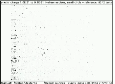
Fig. 1: Tests with parameters around the Helium nucleus
Force balance is only given with Si = 0. Using this energy-momentum tensor means, there is no choice: The sources mustvanish, with them the divergences of the field tensor
Fia
;a= 0 : (44)
Einstein stated this already in his Four Lectures [7]. This step is possible, as explained.
The necessity of this energy-momentum tensor to have just this form is also derived by Montesinos and Flores [21] based on Noether’s theorem [22], but only without sources.
Numerical simulations according to source-free Einstein-Maxwell equations [18] demonstrate that the areas around possible formal singularities do not exist at all. Also known analytic solutions of Einstein’s equations like the isotropic Schwarzschild solution [7],[19] indicate this. The event hori-zon here is the boundary. In general, a geometric boundary is given when physical components of metrics take an abso-lute value of 1. It is a kind of horizon in any case. We have to suppose it at the conjectural radius of the particle respec-tively nucleus, for chaos from the non-linear field equations (see next section).
However, any additional terms or extended methods can-not really repair the inconsistencies from the sources.
ForT = 0andR = 0, Einstein’s equations now result in
Rik=
1
4 gikFabFab FiaFka
: (45)
Equations (1), (44), and (45) involve a special Rieman-nian geometry of the space-time, as explained in [12] and [20]. The field tensor becomes a curve parameter of the world-lines like the curvature vector.
5 On numerical simulations
The precedingly explained insights are supported by numer-ical simulations according to equations (3), (44), and (45).
Fig. 2: Tests with parameters around the electron
Recent robust results can be seen at [23], including the Pascal code of the used program, and a program visualizing these results.
Algorithms and simulation techniques are discussed in [18], as well as the method of approximating the partial dif-ferential equations by discrete ones. The principle consists in going from the known (e.g. the distant field of a point charge) to the unknown. In this paper, two visualized samples are shown.
The particle quantities like mass, spin, charge, magnetic momentum are integration constants from mentioned tensor equations, and are inserted as parameters into the initial con-ditions. The initial conditions start from point charges, or analogous functions for the other integration constants re-spectively, and are assumed only for great radius.The non-linearities are absolutely negligible at this place.
The number of iterations during the computation up to terminating the actual test means a degree of stability of the solution, and is marked in the graphs as a more or less fat “point”. The reference point (according to literature [24]) is displayed as small circle.
In tests only with mass and charge (remaining parame-ters zero), masses of preferably small nuclei emerge signifi-cantly, together with the right charge at the Helium nucleus, Figure 1.y Unfortunately, the procedure is too inaccurate for the electron mass. In return, the other parameters emerge very significantly, see Figure 2.
Above mentioned stability could have to do with chaos. The author had to take notice of the fact, that the numerical solutions are fundamentally different from analytic solutions. Any singularities from analytic solutions are always replaced by boundaries, which can be interpreted as geometrical limits. The non-linear equations (which behave chaotically) lead
Concrete initial conditions see [23], also [18].
alwaysto these geometrical boundaries, which are 1) finite and 2) outside of possible singular points. Areas with singular points do not exist, i.e. are irrelevant.
One could understand this fundamental contrast by the fact that the differences in time and length are never made zero in a numerical way. The results, exclusively achieved this way, support the view that one has to assume a discrete space-time that does not give reasons for action at a distance. The continuum is only defined with action from point to point, independently on distance or interval between adjacent points.
In order to correctly depict nature, it is apparently nec-essary to take into consideration the deviations, appearing during the calculation with finite differences. In nature ap-parently these deviations do not vanish with the transition to very small differences.
Konrad Zuse asked the question, if the possibility to ar-bitrarily subdivide quantities is “conceivable at all” in na-ture [25]. Common imagination of a consequent quantization leads to the problem of privileged coordinates, or a privileged frame [25]. Nature has never indicated it. However, it is suc-cessful practice in electrical engineering to adapt the coor-dinates to the actual problem (Wunsch [11]). Linear equa-tions showed to be insensitive to the selection of coordinates. It requires intense research work to prove the chaotic be-haviour of the non-linear equations dependent on the coordi-nates. The author was so fortunate to see the mentioned cor-relations with spherical coordinates. As well, the corcor-relations became highly significant when the raster distances were the same tangentially as well as radially (dr = r d#) just at the conjectural particle radius.
6 Concluding remarks
If the obtained insights are right, all quantum phenomena should be understandable by them. At this place, tunnel ef-fects are mentioned. This example is supplemented with very brief but essential remarks on causality.
6.1 On tunnel effects
Equations (1), (44), and (45) allow structures, in which a fi-nite distance (as the outer observer sees it) can locally become zero, but metrics does not become singular. That were a real tunnel with an “inner” length of zero. An event at the one side is “instantaneously” seen at the other side. A known effect, that could be interpreted this way, is the EPR effect [26, 27]. Such tunnels might arise by accident.
This view is supported with changes of metrics by electro-magnetism. Distances are locally shortened (at electric fields in direction of the field strength), what can lead to a feedback. Trump and van de Graaf have measured the flashover in the vacuum, dependent on the distance of the electrodes (Kapcov
See also the joke with Mozart’s Fortieth symphony by Nimtz.
[28]). As well, the product of voltage and field strength was nearly constant
U E 1013V2m 1: (46)
That means @g11
@r 210 41m 1: (47)
One will not see these tiny changes, but they are appar-ently enough to release lightning etc.
On the whole, the influence of gravitation prevails, so that the space-time is macroscopically stable. Table 1 shows the arithmetical deviations of metrics at a radius of10 15m, that is roughly the conjectural radius of nuclei.
proton free electron
(11)( (44))from mass 2:4810 39 1:3010 42 (11)from charge 1:8510 42 1:8510 42 (34)from spin j2:6010 40 j2:6010 40 (34) from charge times
magn. momentum j5:5710 43 j3:610 40 (33)from magn.
momen-tum (ambiguous) 1:6410 43 6:8410 38
Table 1: The arithmetical deviations of metrics at10 15m.
The influence by mass decreases with1=r, however, that by charge and spin with1=r2, and that by magnetic momen-tum with1=r4.
6.2 On causality
Firstly, equations (3), (44), and (45) provide 10 independent equations for 14 componentsgik; Ai. With it, causality is not given in principle. It is false to claim, a geometric ap-proach would imply causality. Geometry has nothing to do with causality, because causality has not been geometrically defined at all.
If we see something causal, it comes from approximations by wave equations, as precedingly explained. These provide close solutions.
Appendix
“Classical” electric and magnetic fields in the vacuum are joined to an antisymmetric tensor of 2nd rank
D = "0E =j0 12
0 @ FF(14)(24)
F(34) 1 A ;
B = 0H = "0 12
0 @ FF(23)(31)
F(12) 1
Current density and charge density result in a source vec-torS
J = c0 12
0 @ SS(1)(2)
S(3) 1
A ; = j0 12S(4): (49)
The indices in parentheses stand for physical components. See also K¨astner [8].
Acknowledgement
The author owes interesting, partly controversy discussions, throwing light upon, to a circle with the gentlemen Prof. Man-fred Geilhaupt, Wegberg (Germany), Dr. Gerhard Herres, Paderborn (Germany), and the psychologist Werner Mikus, K¨oln (Cologne, Germany). Special thanks are due to Prof. Arkadiusz Jadczyk, Castelsarrasin (France), who accompa-nied the article with critical questions and valuable hints, and Dr. Horst Eckardt, M¨unchen (Munich, Germany), who care-fully looked over this paper.
Submitted on February 19, 2009/Accepted on February 23, 2009
References
1. Siegel W. Fields. arXiv: hep-th/9912205.
2. Wilczek F. Quantum field theory.Review of Modern Physics, 1999, v. 71, 85–S95; arXiv: hep-th/9803075.
3. Roy D.P. Basic constituents of matter and their interactions — a progress report. arXiv: hep-ph/9912523.
4. ’t Hooft G. The conceptual basis of quantum field theory. Lec-tures given at Institute for Theoretical Physics, Utrecht Uni-versity, and Spinoza Institute, Utrecht, the Netherlands, 2005, http://www.phys.uu.phys.nl/˜thooft/lectures/basisqft.pdf
5. Geilhaupt M. Private information, 2008. See also: Geilhaupt M. and Wilcoxen J. Electron, universe, and the large numbers between. http://www.wbabin.net/physics/mj.pdf
6. Price J.C. et al. Upper limits to submillimetre-range forces from extra space-time dimensions.Nature, 2003, v. 421, 922–925.
7. Einstein A. Grundz¨uge der Relativit¨atstheorie. (A back-translation from the Four Lectures on Theory of Relativity.) Akademie-Verlag Berlin, Pergamon Press Oxford, Friedrich Vieweg & Sohn Braunschweig, 1969.
8. K¨astner S. Vektoren, Tensoren, Spinoren. Akademie-Verlag, Berlin, 1960.
9. Bruhn G.W. Gauge theory of the Maxwell equations. Fachbereich Mathematik der TU Darmstadt, http://www. mathematik.tu-darmstadt.de/˜bruhn/Elektrodynamik.html
10. Bruhn G.W. Zur Rolle des magnetischen Vektorpoten-tials beim Aharonov-Bohm-Effekt. Fachbereich Mathematik der TU Darmstadt, http://www.mathematik.tu-darmstadt.de/ ˜bruhn/Elektrodynamik.html
11. Wunsch G. Theoretische Elektrotechnik. Lectures at Tech-nische Universit¨at Dresden, 1966–1968.
12. Bruchholz U. Zur Berechnung stabiler elektromagnetischer Felder. Z. elektr. Inform.- u. Energietechnik, Leipzig, 1980, v. 10, 481–500.
13. Reichardt W. Physikalische Grundlagen der Elektroakustik. Teubner, Leipzig, 1961.
14. Skudrzyk E. Die Grundlagen der Akustik. Wien, 1954. 15. Lenk A. Ausgew¨ahlte Kapitel der Akustik. Lectures at
Tech-nische Universit¨at Dresden, 1969.
16. Bruchholz U. Berechnung elementarer Felder mit Kontrolle durch die bekannten Teilchengr¨oßen. Experimentelle Technik der Physik, Jena, 1984, v. 32, 377–385.
17. Bruchholz U. Derivation of Planck’s constant from Maxwell’s electrodynamics. http://bruchholz.psf.net/h-article.pdf; http:// UlrichBruchholz.homepage.t-online.de/HomepageClassic01/ h-article.pdf
18. An obsolete report is to find at http://bruchholz.psf.net or http:// UlrichBruchholz.homepage.t-online.de; See also a German-language textbook, Chapter 4.
19. Eisenhart L.P. Riemannian geometry. Princeton university press, 1949.
20. Bruchholz U. Ricci main directions in an EM vacuum. 2001. Look for improved articles at http://bruchholz.psf.net; http:// UlrichBruchholz.homepage.t-online.de
21. Montesinos M. and Flores E. Symmetric energy-momentum tensor in Maxwell, Yang-Mills, and Proca theories obtained us-ing only Noether’s theorem. arXiv: hep-th/0602190.
22. Noether E. Invariante Variationsprobleme. Nachr. d. K¨onig. Gesellsch. d. Wiss. zu G¨ottingen, Math-phys. Klasse, 1918, 235–257 (English translation by M. A. Tavel in: Transport Theory and Statistical Physics, 1971, v. 1(3), 183–207; arXiv: physics/0503066).
23. Recent visible data are in the packages http://www.bruchholz-acoustics.de/robust.tar.gz; http://UlrichBruchholz.homepage.t-online.de/HomepageClassic01/robust.tar.bz2
24. The author took the reference values from: Gerthsen Ch. Physik. Springer-Verlag, Berlin-Heidelberg-New York, 1966 (regularly updated lists of the particle numbers are to find at http://pdg.lbl.gov/)
25. Zuse K. Rechnender Raum.Elektronische Datenverarbeitung, 1967, v. 8, 336–344; see also ftp://ftp.idsia.ch/pub/juergen/ zuse67scan.pdf
26. Einstein A., Podolsky B., and Rosen N. Can quantum-mechanical description of physical reality be considered com-plete?Phys. Rev., 1935, v. 47, 777–780.
27. Zeilinger A. Von Einstein zum Quantencomputer.Neue Z¨urcher Zeitung, v. 72, Nr. 148 vom 30.06.1999.