Joint dynamic probabilistic constraints with
projected linear decision rules
Vincent Guigues FGV/EMAp,
22250-900 Rio de Janeiro, Brazil [email protected]
Ren´e Henrion
Weierstrass Institute Berlin 10117 Berlin, Germany [email protected]
Abstract
We consider multistage stochastic linear optimization problems combining joint dynamic probabilistic constraints with hard constraints. We develop a method for projecting decision rules onto hard constraints of wait-and-see type. We establish the relation between the original (infinite dimensional) problem and approximating problems working with projections from different subclasses of decision policies. Con-sidering the subclass of linear decision rules and a generalized linear model for the underlying stochastic process with noises that are Gaussian or truncated Gaussian, we show that the value and gradient of the objective and constraint functions of the approximating problems can be computed analytically.
Keywords dynamic probabilistic constraints, multistage stochastic linear programs, lin-ear decision rules.
1
Introduction
A probabilistic constraint is an inequality
P(g(x, ξ)≤0)≥p, (1)
where g is a mapping defining a random inequality system, x is a decision vector, and ξ is a random vector living on a probability space (Ω,A,P). In many applications, the decision x has to be taken before the realization of the random parameter ξ is observed (’here-and-now decisions’). The meaning of (1) is the following: a decision x is feasible if and only if the random inequality system g(x, ξ) ≤ 0 is satisfied at least with prob-ability p ∈ (0,1]. Choosing p close to one reflects the wish for robust decisions which moreover can be interpreted in a probabilistic way. Probabilistic constraints have impor-tant applications in engineering optimization problems involving uncertain data, e.g., in water management, telecommunications, electricity network expansion, mineral blending, chemical engineering, etc. For a comprehensive overview on the theory, numerics and applications of probabilistic constraints, we refer to, e.g., [4, 13].
Often, decisions may depend on time, i.e., the vector x represents a discrete decision process. In such case, the ’here-and-now’ setting of (1) means that decisions for the whole time period are taken prior to observing the random parameter, which is now a discrete
stochastic process. Then, inequality (1) represents a static probabilistic constraint because the decision process does not take into account the gain of information over time while observing the random process. To overcome this deficiency, one may pass from a decision vectorx= (x1, . . . , xT) to a closed loop decision policy
x= (x1, x2(ξ1), x3(ξ1, ξ2), . . . , xT(ξ1, . . . ξT−1))
each component of which represents a function of previously observed values of the ran-dom process for a given time. With this definition, (1) becomes a dynamic probabilistic constraint now acting on a variable x from an infinite dimensional space. In order to return to a numerically tractable problem in finite dimensions, the decision policies are often parameterized, the most common approach being the introduction of linear decision rules, i.e., xi(ξ) = Aξ+b for appropriate A, b which now become the finite-dimensional
substitutes for the originally infinite dimensional variables. This strategy has been in-troduced to probabilistically constrained hydro reservoir problems as early as 1969 [15]. It was used there (and in subsequent publications) in the context of so-called individual probabilistic constraints where each component of the given random inequality system is individually turned into a probabilistic constraint:
P(gi(x, ξ)≤0)≥p (i= 1, . . . , m).
The big advantage of such individual constraints is that - in case the component gi(x, ξ)
is separable with respect to ξ - they are easily converted into explicit constraints via quantiles. In particular, if g happens to be a linear mapping and the objective is linear too, then all one has to do to solve such a probabilistic optimization problem is to apply linear programming. It is well known, however, that the chosen probability level p in an individual model may by far not correspond to the level in a joint model, given by (1), where the probability is taken over the entire inequality system. In [19] a hydro reservoir problem is presented where at an optimal release policy the level constraints are satisfied in each time interval with probability 90% individually, whereas the probability of keeping the level constraints through the whole time period is as low as 32%. This observation strongly suggests to deal with the joint model (1) albeit much more difficult to treat algorithmically.
The aim of the current paper is to discuss several modeling issues in the context of dynamic probabilistic constraints putting the emphasis on
• joint probabilistic constraints as in (1);
• continuous multivariate distributions of the random vector (in particular, Gaussian) with typically correlated components;
• parameterized decision rules (in particular, linear and projected linear ones);
• mixed probabilistic and hard (almost sure) constraints.
We do not intend to investigate the so-called time consistent models for dynamic proba-bilistic constraints as it was done, for instance, in [2]. Moreover, the focus of this paper is not to develop a new algorithm neither the study of a concrete application, although a simple hydro reservoir problem will guide us as an illustration. Our idea is rather to provide a modeling framework taking into account the items listed above and yielding a link to algorithmic approaches for static probabilistic constraints. The latter have been successfully dealt with numerically in the context of linear probabilistic constraints under multivariate Gaussian (and Gaussian like) distribution (see, e.g., [13, 14, 19, 20]).
The paper is organized as follows: Section 2 presents a general linear multistage prob-lem with probabilistic and hard constraints. It describes a method for projecting decision rules onto hard constraints of wait-and-see type. It finally establishes the relation be-tween the original (infinite dimensional) problem and approximating problems working with projections from different subclasses of decision policies. These subclasses are kept very general in this section while they are specialized to linear decision rules in Section 3. In that same section the probabilistic time series model we intend to use for the dis-crete stochastic process is made precise. It is clarified, how the objective, the probabilistic constraint and the hard constraints look like under this probabilistic model and the as-sumed linear decision rules. Finally, Section 4 explicitly develops the shape of general optimization problems introduced in Section 2 when assuming multivariate Gaussian and truncated Gaussian models for the discrete process. Advantages and difficulties for the different problems are discussed.
2
A linear multistage problem with probabilistic constraints
2.1 The general model
For givenT ∈NwithT ≥2, we consider aT-stage stochastic linear minimization problem with the following random constraints:
t
P
τ=1
At,τyτ+ t
P
τ=1
Bt,τξτ ≤bt, t= 1, . . . , T. (2)
Here, for t= 1, . . . , T, yt are nt-dimensional decision vectors, ξt are Mt-dimensional
ran-dom vectors, At,τ and Bt,τ are given matrices of orders (lt, nτ) and (lt, Mτ), respectively,
and bt ∈ Rlt are given vectors. In what follows, the index ’t’ will be interpreted as time
and yt and ξt represent discrete decision and stochastic processes, respectively, having
random process have the same dimensionM1 =· · ·=MT =:M. The joint random vector
ξ = (ξ1. . . , ξT) ∈ RM T is supposed to live in a probability space (Ω,A,P). Similarly to
traditional multistage stochastic programming, we shall assume that the decision yt is
taken in the beginning of time interval [t, t+ 1) but the random vectorξtis observed only
at the end of that same interval. Therefore, the realization of ξt is unknown at the time
one has to decide on yt. On the other hand, in order to take into account the gain of
in-formation due to past observations of randomness, the decisionytis allowed to depend on
ξ1:t−1:= (ξ1, . . . , ξt−1) such that yt is Borel measurable. In the following, we will refer to
theyt(ξ1:t−1), t= 1, . . . , T, (including the deterministic first stage decisiony1(ξ1:0) :=y1)
as decision policies rather than decision vectors in order to emphasize their functional character. Summarizing, we are dealing with the following problem:
minimize EPT
t=1hht, yt(ξ1:t−1)i subject to
t
P
τ=1
At,τyτ(ξ1:τ−1) +
t
P
τ=1
Bt,τξτ ≤bt, t= 1, . . . , T, (3)
whereE is the expectation operator.
Example 2.1 As an illustration, we consider a two-stage problem for the optimal release
y of a hydro-reservoir under stochastic inflow ξ. The released water is used to produce and sell hydro-energy at a price p which is assumed to be known in advance. Given the two stages, these quantities have components ξ = (ξ1, ξ2), p = (p1, p2), y = (y1, y2(ξ1)).
The reservoir level is required to stay at both stages between given lower and upper limits
ℓlo, ℓup, respectively. Finally, the release is supposed to be bounded by fixed operational limits ylo, yup, respectively, for turbining water at both time stages. Denoting by ℓ0 the
initial water level in the reservoir, the random cost is given by −(p1y1 +p2y2(ξ1)) while
the random constraints can be written
ℓlo≤ℓ0+ξ1−y1≤ℓup
ℓlo≤ℓ
0+ξ1+ξ2−y1−y2(ξ1)≤ℓup
ylo≤y1≤yup
ylo≤y2(ξ1)≤yup.
(4)
It is easy to see that this is a special instance of problem (3) with data
h:=−p, A1,1:=A2,2 :=
−1 1 1 −1
, A2,1 :=
−1 1 0 0
,
B1,1 :=B2,1 :=B2,2 :=
1 −1 0 0
, b1:=b2 :=
ℓup−ℓ
0
ℓ0−ℓlo
yup −ylo
.
be required to hold almost surely, thus yielding very robust decisions avoiding violation of constraints with probability one. In that case, we obtain the well-defined optimization problem
minimizeEPT
t=1hht, yt(ξ1:t−1)i subject to
t
P
τ=1
At,τyτ(ξ1:τ−1) +
t
P
τ=1
Bt,τξτ ≤bt t= 1, . . . , T, P-almost surely. (5)
If in the constraints of (5) one had thatBT,T = 0, then the last componentξT of the random
process would not enter the constraints and (5) would represent a conventional multistage stochastic linear program. Note, however, thatB2,26= 0 in the two-stage problem (4) and
so the random inflow ξ2 observed only after taking the last decision y2(ξ1) plays a role
in some of the (level) constraints. In such cases, insisting on almost sure satisfaction of constraints may be impossible in particular for unbounded random distributions. In (4), for instance, no matter what has been observed (ξ1) or decided on (y1,y2(ξ1)) until the
beginning of the second time interval, the last unknown inflow ξ2 could always be large
enough to eventually violate the upper level constraint
ℓ0+ξ1+ξ2−y1−y2(ξ1)≤ℓup.
Therefore, one has to look for alternative models for such constraints leaving the possibility of a ’controlled’ violation. These observations lead us to distinguish in (5) between hard constraints which have to be satisfied almost surely for physical or logical reasons and
soft constraints which can be dealt with in a more flexible way. A typical example for hard constraints are the lower and upper limits for the amounts of turbined water (ylo≤ y1, y2(ξ1)≤yup) in (4): there is no turbining beyond the given operational limits just for
physical reasons.
On the other hand, the reservoir level constraints could be considered to be soft ones. Suppose, for instance, that ℓlo in (4) represents the physical lower limit of the reservoir below which no water is released and turbined. Then, a violation of the lower level constraint can never happen and so the corresponding two inequalities can be removed from (4). Doing so, one has to take into account, however, that not the total amount of the release policiesy1 andy2(ξ1), respectively, can be turbined and sold at the given prices
but only the part not violating the lower level constraint, i.e., min{y1, ℓ0+ξ1−ℓlo}in the
first stage and min{y2(ξ1), ℓ0 +ξ1+ξ2−llo−y1} in the second stage. This means that
the original profitsp1y1 andp2y2(ξ1) at the two stages have to be reduced by the amounts
p1 y1−ℓ0−ξ1+ℓlo+ and p2 y2(ξ1)−ℓ0−ξ1−ξ2+ℓlo+y1+, respectively, where the
lower index ’+’ as usual represents the component-wise maximum of the given expression and zero. In this way, the original lower level constraints in (4) have been removed and compensated for by appropriate penalty terms in the objective.
Next, suppose that ℓup in (4) represents some upper limit of the reservoir which is considerably lower than the physical one and serves the purpose of keeping a flood reserve. Then we may neither be able to satisfy this upper limit almost surely (see above) nor to remove it in exchange for an appropriate penalty. In such cases it is reasonable to impose a probabilistic constraint instead:
where p ∈ (0,1) is a specified probability level. Hence, the release policies y1, y2(ξ1) are
defined to be feasible if the indicated set of random inequalities is satisfied at least with probability p. Observe that p = 1 would yield the almost sure constraints again, hence choosing p close to but smaller than one, offers us the possibility of finding a feasible release policy while keeping the soft upper level constraint in a very robust sense.
Example 2.2 Taking into account all three kinds of hard and soft constraints in the (ran-dom) hydro reservoir model (4), one ends up with the following well-defined optimization problem:
minimize
−E(p1y1+p2y2(ξ1))
+E(p1(y1−ℓ0−ξ1+ℓlo)++p2(y2(ξ1)−ℓ0−ξ1−ξ2+y1+ℓlo)+)
(6)
subject to
P
ℓ0+ξ1−y1 ≤lup
ℓ0+ξ1+ξ2−y1−y2(ξ1)≤ℓup
≥p
ylo≤y
1 ≤yup
ylo ≤y2(ξ1)≤yup
P-almost surely.
Here, the group of soft lower level constraints has disappeared and entered the objective as a second penalization term, the group of soft upper level constraints (for which no penalization costs are available) has turned into a probabilistic constraint and the group of hard box constraints is formulated in the almost sure sense.
Applying this strategy to the general random constraints (5), we are led to partition the data matrices and vectors for t= 1, . . . , T, and τ = 1, . . . , t, as
At,τ =
A(1)t,τ, A(2)t,τ, A(3)t,τ, Bt,τ =
B(1)t,τ, Bt,τ(2), B(3)t,τ, bt=
b(1)t , b(2)t , b(3)t
according to penalized soft constraints (upper index (1)), probabilistic soft constraints (upper index (2)) and almost sure hard constraints (upper index (3)). Accordingly, (5) turns into the well-defined optimization problem
minimize (7)
T
P
t=1
E (
hht, yt(ξ1:t−1)i+
*
Pt,
t P
τ=1
A(1)t,τyτ(ξ1:τ−1) +
t
P
τ=1
Bt,τ(1)ξτ −b(1)t
+
+)
subject to
P t
P
τ=1
A(2)t,τyτ(ξ1:τ−1) +
t
P
τ=1
Bt,τ(2)ξτ ≤b(2)t , t= 1, . . . , T
≥p
t
P
τ=1
A(3)t,τyτ(ξ1:τ−1) +
t
P
τ=1
Bt,τ(3)ξτ ≤b(3)t , t= 1, . . . , T, P-almost surely.
Here, the Pt ≥ 0 refer to a cost vectors penalizing the violation of soft constraints with
2.2 Projection onto hard constraints of wait-and-see type
We will refer in (5) to wait-and-see constraints if Bt,t = 0 for all t = 1, . . . , T, and to
here-and-now constraints otherwise. The distinction is made according to whether in the constraint of any stage t there is unobserved randomness ξt left or not. For example, in
(4), the first two inequalities (level constraints) are here-and-now whereas the last two (operational limits) are wait-and-see. As mentioned earlier, the almost sure constraints in (7) don’t have a good chance to be ever satisfied if BT,T(3) 6= 0 and the support of the random distribution is unbounded. We’ll get back to such here-and-now constraints for bounded support of the random distribution in Section 4.5. First, let us deal with the case where all hard constraints are of wait-and-see type as in (6). In this case, owing to Bt,t(3) = 0 for allt= 1, . . . , T, the constraint set of (7) can be written as
M1:=
n
(yt(ξ1:t−1))t=1,...,T| (8)
P
t
X
τ=1
A(2)t,τyτ(ξ1:τ−1) +
t
X
τ=1
Bt,τ(2)ξτ ≤b(2)t , t= 1, . . . , T
!
≥p
t
X
τ=1
A(3)t,τyτ(ξ1:τ−1) +
t−1
X
τ=1
Bt,τ(3)ξτ ≤b(3)t , t= 1, . . . , T, P-almost surely
o .
In the context of numerical solution approaches, one will usually not work in the infinite-dimensional setting of all Borel measurable policies but rather with a finite infinite-dimensional approximation which may be defined by some proper subset K of policies. Later in this paper we will deal with the class of linear decision rules (see Section 3.2). The feasible set of (7) will then become the intersectionM1∩ Krather than justM1. This intersection
may turn out to be very small or even empty thus leading to a poor approximation of the infinite dimensional problem (7). If, for instance one of the hard constraints is given as y2(ξ1)∈[1,2] (P-almost surely) and if, moreover, the class of policies is
K:={(y1, y2(ξ1)|∃a∈R:y2(ξ1) =aξ1},
then, clearly,M1∩ K=∅. One possibility to avoid this kind of problem is to operate with
projections of policies onto the feasible domain of hard constraints.
Given a closed convex subset X of a finite dimensional space, we denote the uniquely defined projection onto this set byπX. Fort= 1, . . . , T, we introduce the multifunctions
Xt(z1:t−1, ξ1:t−1) :=
(
y|A(3)t,ty(ξ1:t−1)≤b(3)t − t−1
X
τ=1
Bt,τ(3)ξτ − t−1
X
τ=1
A(3)t,τzτ(ξ1:τ−1)
)
. (9)
Here, we adopt the previous notationz1:t−1 := (z1, . . . , zt−1) fromξ. By Π we denote the
operator which maps a policy y := (yt(ξ1:t−1))t=1,...,T to a new policy z := Π(y) defined
iteratively by
zt(ξ1:t−1) :=πXt(z1:t−1,ξ1:t−1)(yt(ξ1:t−1)) ∀ξ, ∀t= 1, . . . , T, (10)
starting from z1 :=πX1(y1). For example, fort= 1,2,3, . . . one gets successively that
z1 : =πX1(y1),
z2(ξ1) : =πX2(z1,ξ1)(y2(ξ1)), ∀ξ1,
so that Π(y) is correctly defined and by (9) satisfies the hard (almost sure) constraints of (7). (10) amounts to a scenario-wise projection onto the polyhedra (9) which can be carried out numerically by solving a convex quadratic program subject to linear constraints. In the special case of rectangular sets [ylo, yup], which can be modeled as a hard constraint in (8) by putting fort= 1, . . . , T and τ = 1, . . . , t−1:
A(3)t,t := (I,−I)T, b(3)t :=
yupt −ytlo
, A(3)t,τ := 0, Bt,τ(3) := 0, (11)
an explicit formula can be exploited: projection of a policy then just means cutting it off at the given lower and upper limits. For instance, in the context of the hard constraints in (6), one has that
Π(y) = Π(y1, y2(·)) =
max{ylo,min{y1, yup}},max{ylo,min{y2(·), yup}}
. (12)
As mentioned above, projection via Π is a way to enforce the hard constraints. This offers several alternatives to the above-mentioned direct intersection of feasible policies fromM1 with a given (typically finite-dimensional) subclass K. One option would consist
in working from the very beginning with projected policies so that the feasible set would become M1 ∩Π(K) rather than M1 ∩ K. Indeed, we shall see in Lemma 2.3 that the
intersection with the original infinite-dimensional feasible set may be substantially larger by doing so (in particular it would be no more empty in the example discussed before). A second option would consist in relaxing the hard constraints to probabilistic constraints similar to the ones given from the beginning and projecting them afterwards onto the set defined by hard constraints. We formalize this idea by introducing the alternative (infinite-dimensional) constraint set
M2:=
n
(yt(ξ1:t−1))t=1,...,T| (13)
P
t
P
τ=1
A(2)t,τyτ(ξ1:τ−1) +
t
P
τ=1
Bt,τ(2)ξτ ≤b(2)t t
P
τ=1
A(3)t,τyτ(ξ1:τ−1) +
t−1
P
τ=1
Bt,τ(3)ξτ ≤b(3)t
t= 1, . . . , T
≥p
o .
We shall see in Lemma 2.3 that the projection ofM2 onto the hard constraints yields the
set M1, so there is no difference in the solution of (7) in the original infinite-dimensional
setting. When considering intersections with a subclassK, however, a significant advantage over working withM1 may be observed.
2.3 Approximating the original problem by means of subclasses of de-cision rules
The following result clarifies the relations between the feasible sets M1, M2 introduced
above and their intersection with (projections of) subclasses of decision rules:
Lemma 2.3 If K is an arbitrary subset of Borel measurable policies (yt(ξ1:t−1))t=1,...,T,
then the following chain of inclusions holds true:
In particular, by setting K equal to the space of all Borel measurable policies, we derive thatΠ(M2) =M1.
Proof. Letz∈M1∩K. Then, the probabilistic constraint for the first and the almost sure
constraints for the other inequality system in (8), respectively, guarantee that the joint probabilistic constraint in (13) is satisfied, hencez∈M2∩ K. Withz fulfilling the almost
sure constraints in (8), we have that z = Π(z), whence z ∈Π(M2∩ K). This proves the
first inclusion in the above chain. Next, as for the second inequality, letz ∈Π(M2∩ K),
hencez= Π(y) for somey ∈M2∩ K. In particular,z∈Π(K) and it remains to show that
z∈M1. As an image of the mapping Π,z satisfies the almost sure constraints of (8). By
y∈M2 and (13), there exists a measurable set S⊆Ω such thatP(S)≥p and
t
X
τ=1
A(2)t,τyτ(ξ1:τ−1(ω)) +
t
X
τ=1
B(2)t,τξτ(ω) ≤ b(2)t
t
X
τ=1
A(3)t,τyτ(ξ1:τ−1(ω)) +
t−1
X
τ=1
B(3)t,τξτ(ω) ≤ b(3)t
are satisfied for all t = 1, . . . , T and all ω ∈ S. By (10), the second inequality system implies (successively for tfrom 1 to T) that
yt(ξ1:t−1(ω))∈Xt(z1:t−1, ξ1:t−1(ω)) ∀t= 1, . . . , T, ∀ω ∈S.
Hence, again by (10), (zt(ξ1:t−1) (ω))t=1,...,T = (yt(ξ1:t−1) (ω))t=1,...,T for allω ∈S.
There-fore, the first inequality system above can be written as
t
X
τ=1
A(2)t,τzτ(ξ1:τ−1(ω)) +
t
X
τ=1
Bt,τ(2)ξτ(ω)≤b(2)t ∀t= 1, . . . , T, ∀ω∈S.
Since P(S)≥p it follows thatz satisfies the probabilistic constraint in (8). Summarizing we have shown that also z∈M1, whence the desired inclusion follows. The last inclusion
is trivial.
The previous Lemma suggests to consider the following 4 optimization problems each of them being some relaxation of our original optimization problem (7):
min{h(y)|y ∈M1∩ K}, (14)
min{h(z)|z∈Π(arg min{h(y)|y∈M2∩ K})}, (15)
min{h(y)|y ∈Π(M2∩ K)}, (16)
min{h(y)|y ∈M1∩Π(K)}. (17)
Herehrefers to the objective function of (7) andK is a given subclass of decision policies. The meaning of (14), (16) and (17) is clear and relates to the feasible sets considered in Lemma 2.3. In (15) we determine first the solution(s) of the inner optimization problem min{h(y)|y ∈M2∩ K} and then project them via Π. If this inner optimization problem
smallest value of the objective. We observe that (16) has the same optimal value as the problem
min{h(Π(y))|y∈M2∩ K}, (18)
where the projection is shifted from the constraints to the objective, and thatyis a solution of (18) if and only if Π(y) is a solution of (16). Hence, (16) and (18) are equivalent and it may be a matter of convenience which of the two forms is preferred. The potential advantage of (15) say over (16) and (17) is that projections don’t have to be dealt with in the constraints or in the objective directly but can be carried out after solving the problem.
Lemma 2.4 Denote byϕ1, ϕ2, ϕ3, ϕ4, respectively, the optimal values of problems
(14)-(17) and by ϕ the optimal value of the originally given problem (7). Then, any solution of problems (14)-(17) is feasible for problem (7) and it holds that
ϕ1, ϕ2 ≥ϕ3≥ϕ4 ≥ϕ.
Proof. From Lemma 2.3 we see that any feasible point and, hence, any solution of (14), (16) and (17) is feasible for (7). From the inclusions of Lemma 2.3 it follows that ϕ1≥ϕ3 ≥ϕ4 ≥ϕ. Now, letz∗ be a solution of (15). Then, there exists somey∗ ∈M2∩ K
such that z∗ = Π (y∗) and y∗ solves the problem min{h(y)|y ∈ M2 ∩ K}. In particular,
z∗ ∈Π (M2∩ K) is feasible for (16). This implies firstz∗ ∈M1 by Lemma 2.3 and, hence,
the asserted feasibility of z∗ for (7). Second, it implies the desired remaining relation ϕ2=h(z∗)≥ϕ3.
Lemma 2.4 can be interpreted as follows: Problem (14) reflects the pure transition to a subclass K of policies in the originally given problem (7). The resulting loss in optimal value equals ϕ1−ϕ ≥0. In contrast, using projections onto hard constraints in the one
or other way as in (16) and (17) may lead to smaller losses in the optimal values. Of course, this advantage of working with projections requires that the computational gain by passing to an interesting subclassKis not destroyed by the projection procedure. This is why in Section 3.2 we shall introduce the class of linear decision rules as a suitable one harmonizing well to a certain degree with projections onto polyhedral sets. The following example illustrates Lemma 2.4:
Example 2.5 Consider the following problem with policies y1, y2(ξ1) as variables:
min y1 subject to
P(ξ1 ≤y1, ξ2 ≤y2(ξ1))≥p
y1, y2(ξ1)∈[0,1], P−almost surely.
We assume that the random vector ξ= (ξ1, ξ2) follows a uniform distribution over the set
Θ = ([−1,1]×[0,1])∪([0,1]×[0,−1]) and that p = 1/3. As a subclass of policies, we consider (purely) linear second stage decisions:
• Solution of the original problem (7):
We claim that the optimal valueϕof the original problem equals0. Indeed, it cannot be smaller than 0 due to the constraint y1 ≥ 0. On the other hand, y1 := 0 and
y2(ξ1) := 1for allξ1 represents a feasible policy because it clearly satisfies the almost
sure constraints and the set ofξ satisfyingξ1 ≤0 and ξ2≤1covers one third of the
support of ξ. Hence the probabilistic constraint is satisfied too. The objective value associated with this feasible policy equals y1= 0, so ϕ= 0 as asserted.
• Solution of problem (14):
The feasible set here is M1∩ K and a feasible second stage policy y2(ξ1) =aξ1 has
to be trivial (a= 0) in order to satisfy the almost sure constraint 0 ≤ y2(ξ1) ≤ 1.
Then, the only choice for y1 such that (y1,0) satisfies the probabilistic constraint is
y1 := 1 (only then, the set ofξ satisfying ξ1 ≤y1 andξ2 ≤0 covers one third of the
support of ξ). Hence the feasible set in this problem reduces to a singleton and its optimal value equals to the objective value of this singleton: ϕ1=y1= 1.
• Solution of problems (15) and (16):
As stated above, (16) is equivalent with (18). In our example, h is the projection onto the first component, hence we seek to minimize (Π(y))1 over the constraint set
M2∩ K = {(y1, aξ1)|a≥ −1,P(y1, aξ1 ∈[0,1], ξ1≤y1, ξ2≤aξ1)≥1/3}
= {(y1, aξ1)|y1∈[0,1], a≥ −1, ψ(y1, a)≥1/3} (19)
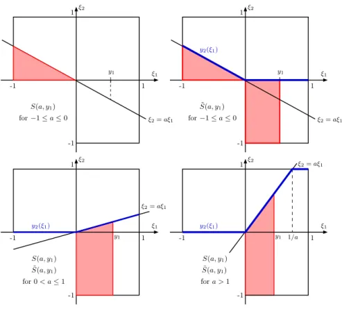
where ψ(y1, a) :=P((ξ1, ξ2)∈ S(a, y1)) with
S(a, y1) :={(ξ1, ξ2)∈Θ|ξ1≤y1, ξ2 ≤aξ1,0≤aξ1 ≤1}
(see Figure 1). Note that in (19) we were allowed to extract the deterministic con-straint y1 ∈[0,1] from the probabilistic constraint.
As (Π(y))1 is the projection of y1 onto the first stage almost sure constraint set
X1 = [0,1] (see (10) and (9)), we get that(Π(y))1=y1. Consequently, according to
(18), we want to minimizey1 for all policies(y1, aξ1)belonging to (19). We consider
three cases:
(i) For −1≤a≤0 (see top left in Figure 1), we have ψ(y1, a) =−a/6<1/3.
(ii) For 0< a≤1 (see bottom left in Figure 1), we have ψ(y1, a) = 13(y1+ay12/2).
The smallest value of y1 satisfying ψ(y1, a)≥1/3 is obtained taking a= 1 and
y1 =−1 +√3>2/3.
(iii) For a >1 (see bottom right in Figure 1), we get
ψ(y1, a) =
1
3(y1+ay12/2) ify1 ≤1/a, 1
2a otherwise.
In particular, ψ(23,32) = 13. We distinguish the two subcases:
(1) a > 3/2: if y1 > 1/a then ψ(y1, a) = 21a < 13 and if 0 ≤ y1 ≤ 1a then
ξ1
ξ2
-1
-1 1
1
S(a, y1)
for−1≤a≤0 ξ2=aξ1
y1 ξ1
ξ2
-1
-1 1
1
˜
S(a, y1)
for−1≤a≤0 ξ2=aξ1
y1
y2(ξ1)
ξ1
ξ2
-1
-1 1
1
ξ2=aξ1
y1
S(a, y1)
˜
S(a, y1)
for 0< a≤1
y2(ξ1) ξ1
ξ2
-1
-1 1
1
1/a y1
S(a, y1)
fora >1 ˜
S(a, y1)
ξ2=aξ1
y2(ξ1)
Figure 1: Representations of S(a, y1) and ˜S(a, y1): top figures for −1 ≤ a ≤ 0, bottom
left for 0< a≤1, and bottom right for a >1.
(2) 1≤a≤3/2: If0≤y1 < 23 theny1 ≤1/a and, hence,
ψ(y1, a)<
1 3
2 3+
3 2
4 2·9
= 1
3
Summarizing, the best value of the objective at an admissible solution of (18) equals
2
3 and is realized uniquely by the optimal policy 23,32ξ1
. The latter is therefore the unique optimal solution of (18). According to our observation above, its projection
Π
2 3,
3 2ξ1
=
2
3,max{0,min{ 3 2ξ1,1}}
(20)
onto the almost sure constraints in our example is an optimal solution of (16). The associated function value equalsh 23,32ξ1= 2/3which therefore is the optimal value
of (16). It follows that ϕ3 = 2/3.
On the other hand, as we have already observed that h(y) = h(Π(y)) = y1 due to
0 ≤ y1 ≤ 1, it follows that the unique optimal solution 23,32ξ1 of (18) yields the
unique optimal solution to the problem
at the same time. Hence, its projection onto the almost sure constraints is the already identified solution (20) of problem (16) implying that the optimal value of problem (15) is the same as that of (16): ϕ2 =ϕ3 = 2/3.
• Solution of problem (17): By virtue of (12), the policies belonging to the setΠ(K)
have the form (y1,max{0,min{aξ1,1}}) for somey1 ∈[0,1]and a≥ −1 (see Figure
1). Since these policies already satisfy the almost sure constraints, all one has to add in order to get a policy feasible for (17) is the satisfaction of the probabilistic constraint. Observe that
M1∩Π(K) ={(y1,max{0,min{aξ1,1}})|y1 ∈[0,1], a≥ −1,ψ˜(y1, a)≥1/3}
where ψ˜(y1, a) :=P((ξ1, ξ2)∈S˜(a, y1)) with
˜
S(a, y1) ={(ξ1, ξ2)∈Θ|ξ1≤y1, ξ2 ≤max(0,min(aξ1,1))}
(see Figure 1). For −1≤a≤0 (see Figure 1), we have
˜
ψ(y1, a) =
1 3(y1−
a
2)<ψ˜(1/2,−1) = 1
3 ∀y1<1/2.
For 0 < a ≤ 1 (see bottom left in Figure 1), we have ψ˜(y1, a) = 13(y1 +ay12/2).
The smallest value of y1 satisfying ψ˜(y1, a) ≥ 1/3 is obtained taking a = 1 and y1 =−1 +
√
3>1/2. Finally, for a >1 (see bottom right in Figure 1), we assume thaty1 ≤1/2. Then,
y1>1/a =⇒ ψ˜(y1, a) = 1
3(2y1− 1 2a)<
y1
3 ≤ 1 3
y1≤1/a =⇒ ψ˜(y1, a) = 1
3(y1+
ay12
2 )≤ 1 3(
1 2 +
1 2a)<
1 3.
This means that there is no feasible policy with y1 ≤ 1/2 and a > 1.
Conse-quently, the optimal value of (17) equals ϕ4 = 1/2 and is realized by the policy
(1/2,max{0,min{−ξ1,1}}) which is the projection of the decision rule(1/2,−ξ1)∈
K onto the hard box constraints.
3
Probabilistic Model and Linear decision rules
Example 2.5 has illustrated the different approximating optimization problems with re-spect to the given one (7). In order to formulate these ideas in a practically meaningful framework, one has to specify the probabilistic model for the random vector ξ and a suitable subclassK of decision rules in Lemma 2.3.
3.1 Probabilistic model
We introduce in this section the class of stochastic processes (ξt) we consider. Each
component ξt(m) ofξt follows a linear model of the form
pt(m) X
k=0
αt,k(m)ξt−k(m) =µt(m) + qt(m)
X
k=0
where lags pt(m), qt(m) are nonnegative and depend on time. We assume that for every t, the coefficientsαt,0(m), αt,pt(m)(m), andβt,qt(m)(m) are nonzero.
Finally, the noises are supposed to obey centered Gaussian lawsεt∼ N(0,Σt), pairwise
independent for different time steps. We recall the notation N(µ,Σ) for referring to a multivariate Gaussian distribution with mean µ and covariance matrix Σ. Hence, ε := (ε1, . . . , εT) ∼ N(0,Σ), where Σ is a block-diagonal covariance matrix whose blocks are
the covariance matrices Σt of the componentsεt.
Remark 3.1 We assume that the parameters of model (21) are known. In its full gen-erality, model (21) is not identifiable. Additional assumptions are needed to identify lags pt(m), qt(m) and calibrate the model parameters. As special cases, the identifiable
SARIMA (with constant lags) and Periodic Autoregressive (PAR, with periodic time de-pendent lags) models can be considered.
Using iteratively model equation (21), for each instant t = 1, . . . , T, we can decompose
ξt(m) as a function of noises ε1, . . . , εt and of past observations of the process (ξt) and of
the noises (observations for instants 0,−1,−2, . . .). More precisely, for everyt= 1, . . . , T
and for every component m, we have for ξt(m) a decomposition of the form
ξt(m) =ct(m) + rt(m)
X
k=1
γt,k(m)ξ1−k(m) + st(m)
X
k=1
δt,k(m)ε1−k(m) + t
X
k=1
θt,k(m)εk(m) (22)
for some lagsrt(m) andst(m) that represent the minimal number of past observations of
respectively the stochastic processes (ξt) and (εt) that are necessary to decompose ξt(m)
over its past. This decomposition will be used in the next sections. In this decomposition, the first two sums gather the past realizations of process (ξt) and of the noises. Lemma
5.1 stated and proved in the Appendix, provides the formulae to compute iteratively the coefficients appearing in the decompositions of ξ1(m), ξ2(m), . . . , ξT(m), m = 1, . . . , M,
of the form (22) above. The computation of these coefficients is necessary when one is interested in solving the optimization problems we consider in the next sections when (ξt)
is of the form (21). A similar decomposition for less general models was given in [7], [8]. It is convenient to write (22) in the compact form
ξt= ˜µt+ Θtε (t= 1, . . . , T), (23)
where for eacht= 1, . . . , T,
• µ˜t is a constant vector inRM with component m given by
˜
µt(m) =ct(m) + rt(m)
X
k=1
γt,k(m)ξ1−k(m) + st(m)
X
k=1
δt,k(m)ε1−k(m),
• Θtis the M×M T matrix
Θt= diag(θt,1(1), . . . , θt,1(M)), . . . ,diag(θt,t(1), . . . , θt,t(M)),0M×M(T−t)
3.2 Linear decision rules
As mentioned in Section 2.2 the numerical solution of problem (7) requires to reduce the space of all Borel measurable decision policies to some convenient finite-dimensional subspace. A simple and widely used way to do so consists in considering so-calledlinear decision rulesas policies which are defined as the set
K:={(yt(ξ1:t−1))t=1,...,T | ∃Ft, ft: yt(ξ1:t−1) =Ftξ1:t−1+ft (t= 1, . . . , T)}, (24)
with matrices Ft and vectors ft of appropriate size. Since the first stage decision y1 is
deterministic, we convene about fixingF1:= 0.
3.2.1 The random inequality system under linear decision rules
Under linear decision rules and the probabilistic model (23), our generic random inequality system
t
X
τ=1
At,τyτ(ξ1:τ−1) +
t
X
τ=1
Bt,τξτ ≤bt t= 1, . . . , T (25)
turns into (fort= 1, . . . , T)
t
X
τ=1
At,τFτΘ1:τ−1+Bt,τΘτ
!
| {z }
Ht(x)
ε≤bt− t
X
τ=1
Bt,τµ˜τ− t
X
τ=1
At,τfτ − t
X
τ=1
At,τFτµ˜1:τ−1
| {z }
αt(x)
.
(26) In this system, ε is the transformed random vector, whereas now x := (Ft, ft)t=1,...T
represents a finite-dimensional decision vector approximating the original decision policies (yt(ξ1:t−1))t=1,...,T. With the notation introduced below the corresponding expressions,
we may compactly rewrite (26) in the form
Ht(x)ε≤αt(x) (t= 1, . . . , T), (27)
where the Ht, ht are affine linear mappings of x. When relating these mappings not to
the generic system (25) but to the concrete systems of hard and soft constraints in (7) labeled by upper indices (1), (2), (3), we shall use the corresponding upper indices for the mappings Ht and ht as well.
We observe that, thanks to affine linearity of Ht, ht, the set of x satisfying (27) is
convex for each fixedε.
3.2.2 The objective function under linear decision rules
From (23) andεhaving a centered distribution, it follows that the expectation ofξtequals
˜
µt. Therefore, the objective of our problem (7) takes under linear decision rules the form
T
X
t=1
hht, Ftµ˜1:t−1+fti
| {z }
β1(x)
+
T
X
t=1
*
Pt,E t
X
τ=1
A(1)t,τyτ(ξ1:τ−1) +
t
X
τ=1
Bt,τ(1)ξτ−b(1)t
!
+
where in the definition of β1 we used once more the conventionx:= (Ft, ft)t=1,...T. Now,
applying (27) with upper index (1) referring to the inequality subsystem penalized in the objective, we can rewrite the objective of (7) under linear decision rules as β(x) :=
β1(x) +β2(x), where
β2(x) :=
T
X
t=1
Pt,E
Ht(1)(x)ε−αt(1)(x)
+
Lemma 3.2 β is convex.
Proof. Since β1 is linear, it suffices to check convexity of β2. As mentioned earlier,
the mappings Ht(1), α(1)t are affine linear, whence the mappingHt(1)(x)ε−α(1)t (x) is affine linear in x. In particular, each component of this mapping is convex in x which re-mains true upon passing to its maximum with zero. It follows that the components of EH(1)
t (x)ε−α
(1)
t (x)
+ (depending only onx) are convex. Now, the result follows from
Pt≥0.
For implementation purposes, it is useful to have an analytic expression of the objective function. For this purpose, we need the folloming Lemma:
Lemma 3.3 Let X be a one-dimensional Gaussian random variable distributed according to N(m, σ2) and let a, b∈ R¯ with a≤ b. Then, with Φ referring to the one-dimensional
standard normal distribution function, it holds that
E[max{a,min{X, b}}] = √σ 2π
exp
−(a−m)
2
2σ2
−exp
−(b−m)
2
2σ2
+
(a−m)Φ(a−m
σ ) + (m−b)Φ( b−m
σ ) +b.
Proof. With fX(x) = √21πσexp
−(x−2σm2)2
being the density ofX and with ˜Φ being the associated cumulative distribution function, we have
E[max{a,min{X, b}}] = Z a
−∞
afX(x)dx+
Z b
a
xfX(x)dx+
Z ∞
b
bfX(x)dx =
aΦ(˜ a) + Z b
a
(x−m)fX(x)dx+m
Z b
a
fX(x)dx+b(1−Φ(˜ b)) =
aΦ(˜ a) +
−σ
√ 2π exp
−(x−m)
2
2σ2
b
a
+m( ˜Φ(b)−Φ(˜ a)) +b(1−Φ(˜ b)) =
σ √ 2π exp
−(a−m)
2
2σ2
−exp
−(b−m)
2
2σ2
+ (a−m) ˜Φ(a) + (m−b) ˜Φ(b) +b.
On the other hand, since σ−1(X−m)∼ N(0,1), we have that, for allz,
˜
and the result follows.
The only non-explicit part in our objective function β(x) is the vector of expectations in the definition of β2(x). Itsithcomponent is given by
E[max(X(x),0)] =E[max{0,min{X(x),+∞}]; X(x) :=H(1)
t (x)ε−α
(1)
t (x)
i.
According to the transformation rules of Gaussian distributions, we know that
X(x)∼ N(m, σ2); m:=−(α(1)t (x))i; σ :=
r
Ht(1)(x)Σ[Ht(1)(x)]T ii,
where Σ is the block-diagonal covariance matrix of ε (see Section 3). With these data, Lemma 3.3 can be employed (with a := 0, b := +∞) to make the objective β(x) fully explicit in terms of the initial data of the problem.
3.2.3 Projection of linear decision rules onto hard constraints
The solution of problems (15), (16), (17), (18) is intimately related with the ability to either explicitly or numerically compute projections Π(y) of policies y ∈ K according to (10). In the case of linear decision rules introduced in (24), the projected policyz:= Π(y) is obtained for y= (Ftξ1:t−1+ft)t=1,...,T as the successive (unique) solution of
(scenario-dependent) quadratic optimization problems:
zt(ξ1:t−1) =
argmin
u k
Ftξ1:t−1+ft−uk2
A(3)t,tu≤b(3)t −tP−1 τ=1
B(3)t,τξτ− t−1
P
τ=1
A(3)t,τzτ(ξ1:τ−1),
(28)
∀ξ, ∀t= 1, . . . , T.
Here, starting from t = 1, previously obtained solutions for zτ are plugged in on the
right-hand side of (28). Hence, for instance the first two components ofz are obtained as
z1 = argmin
u
n
kf1−uk2|A(3)1,1u≤b (3) 1
o
z2(ξ1) = argmin
u
n
kF2ξ1+f2−uk2|A(3)2,2u≤b (3)
2 −B
(3)
2,1ξ1−A(3)2,1z1
o ∀ξ1.
In the special case of box constraints
yt(ξ1:t−1)∈[yt, yt] P-almost surelyt= 1, . . . , T, (29)
an explicit formula for the projection ofy= (Ftξ1:t−1+ft)t=1,...,T can be provided:
Π(y) =max{(y
t)i,min{(Ftξ1:t−1+ft)i,(yt)i}}
t=1,...,T;i=1,...,nt
3.2.4 Probabilistic constraints under Linear Decision Rules and Gaussian dis-tribution
Under the assumption of linear decision rules (24), the originally dynamic probabilistic constraint
P
t
X
τ=1
At,τyτ(ξ1:τ−1) +
t
X
τ=1
Bt,τξτ ≤bt t= 1, . . . , T
!
≥p
associated with (25) and occuring in problems (7) turns into a conventional static proba-bilistic constraint
P(Ht(x)ε≤αt(x) (t= 1, . . . , T))≥p, (31)
with finite-dimensional decisionsx := (Ft, ft)t=1,...T. (31) represents a joint linear
proba-bilistic constraint under Gaussian distribution. This class has been intensively studied with respect to its analytical properties and numerical solution approaches, see, e.g., [4, 13]. For an algorithmic treatment of such probabilistic constraints within the framework of nonlinear optimization it is important to have required information about the probability function
ϕ(x) :=P(Ht(x)ε≤αt(x) (t= 1, . . . , T))
defining the inequality constraint ϕ(x) ≥p in (31). In particular, procedures computing or, better, approximating values and gradients of ϕ are needed. As shown in [20], both tasks can be realized simultaneously by reduction to the computation of multivariate Gaussian distribution functions. The latter can be quite efficiently done using Genz’ code as described in [5]. An alternative approach consists in the use of the so-called spheric-radial decomposition of Gaussian random vectors [3, 16, 18]. Another important property for algorithmic purposes is convexity of the feasible set described by (31). While this is well-known to be true in case of constant matrices Ht and mappings αt having concave
components [13, Theorem 10.2.1], the same does not hold true in general for (31), in particular not for arbitrary probability levels p. Apart from special cases, such as the presence of one single random inequality in the system [10, 21] or specially structured covariance matrices [12, 9], where convexity for sufficiently large p could be guaranteed, no general result on this issue seems to be available so far.
4
Approximating optimization problems under Linear
De-cision Rules and Gaussian and truncated Gaussian
distri-bution
4.1 First optimization problem
The first optimization problem we address is (14), i.e., the original problem (7) but with the feasible set intersected with the class of linear decision rules (24). Making recourse to the compact notation introduced in Section 3.2, Problem (14) writes
min{β(x) | P(H(2)
t (x)ε≤α
(2)
In the definition ofα(3)t according to (26) we have to recall thatBt,t(3)= 0 for allt= 1, . . . , T
according to our wait-and-see perspective on hard constraints (see Section 2.2). (32) is a nonlinear optimization problem with a joint probabilistic and a (linear) semi-infinite constraint (P-almost surely could be replaced by ’for P-almost all ε∈Ξ’, where Ξ is the support of the random vector ε).
Proposition 4.1 The hard constraint in problem (32) can be explicitly represented in terms of the original data (see (26)) as the system of linear (in-)equalities fort= 1, . . . , T:
t
X
τ=1
A(3)t,τFτΘ1:τ−1+Bt,τ(3)Θτ
= 0,
t−1
X
τ=1
Bt,τ(3)µ˜τ+ t
X
τ=1
A(3)t,τfτ + t
X
τ=1
A(3)t,τFτµ˜1:τ−1 ≤ b(3)t .
Proof. As mentioned above, the hard constraint in problem (32) can be replaced by
Ht(3)(x)ε≤α(3)t (x) forP-almost allε∈Ξ (t= 1, . . . , T). (33)
Since ε follows a mutivariate Gaussian distribution, its support is the whole space. As a consequence, somexcan be feasible for (33) only ifHt(3)(x) = 0 which in turn implies that
αt(3)(x)≥0. Conversely, any xsatisfying these two relations is feasible for (33). Thus, we have shown that (33) is equivalent with the system Ht(3)(x) = 0, α(3)t (x) ≥0. Now, (26) yields the assertion of the proposition.
By virtue of Proposition 4.1, the hard constraints in (32) define a polyhedral constraint set for the decision vector x. Recalling Lemma 3.2, (32) would be a convex optimization problem provided that the probabilistic constraint defines a convex feasible region. As discussed in Section 3.2.4, this can be guaranteed, however, only in certain special cases. Moreover, the range of applicability of Proposition 4.1 is potentially small:
Corollary 4.2 Assume that all coefficientsθt,kin (22)have all components different from
zero. Then, if the hard constraints in (32) represent simple box constraints, the only feasible linear decision rules are static ones.
Proof. For box constraintsy ∈[ylo, yup], we are dealing with the data specified in (11). Accordingly, the equation derived in Proposition 4.1 yields that
A(3)t,tFtΘ1:t−1+Bt,t(3)Θt= 0 t= 1, . . . , T.
Recalling that, by the assumed wait-and-see structure for the hard constraints, we have
Bt,t(3) = 0 for t= 1, . . . , T (see Section 2.2), and taking into account that A(3)t,t = (I,−I)T, we derive in particular the relationsFtΘ1:t−1 = 0 fort= 1, . . . , T. Now, our assumption on
coefficients θt,k ensures that the matrices Θ1:t−1 are surjective. As a consequence, Ft= 0
fort= 1, . . . , T, which means that the linear decision rules in (24) reduce toyt(ξ1:t−1) =ft
fort= 1, . . . , T. In other words, one is back to a static decision problem.
4.2 Second optimization problem
The second optimization problem to be discussed is (15). We will focus our attention on the inner optimization problem
min{h(y)|y∈M2∩ K}. (34)
If this problem happens to have a unique solution, then its projection via Π onto the hard constraints will be unique and thus will be a solution of the overall problem too. Otherwise, the outer optimization problem in (15) just serves the purpose of selecting the best solution among projected solutions of the inner problem possibly realizing different values of the objective functionh. We will not address the issue of possible non-uniqueness of (34) here.
By (13), and using once more the compact notation of Section 3.2 along with the definition (24) of linear decision rules, problem (34) writes
min{β(x)|P(Ht(2)(x)ε≤α(2)t (x), Ht(3)(x)ε≤α(3)t (x) (t= 1, . . . , T))≥p}. (35)
This problem has the same objective as (32) but the feasible set differs by the absence of hard constraints and the presence of an enlarged inequality system in the joint chance constraint. Once, a solution x∗ of (35) has been determined, it is projected onto the hard constraints (either using an explicit formula if possible or by solving a quadratic optimization problem as described in Section 3.2.3) in order to yield a decision policy Π(x∗) which is feasible for the original infinite-dimensional problem (7).
4.3 Third optimization problem
The third optimization problem we consider is (16) or its equivalent form (18). Observe first, that (16) can be written
min{h(z)|z= Π(y), y ∈M2∩ K}.
The inclusion in the constraint set of this optimization problem is the same as in (34) and can thus be formulated as the probabilistic constraint in (35) under our convention
x := (Ft, ft)t=1,...T . Taking into account formula (28) for the projection z = Π(y), we
arrive at the following description for problem (16):
min{h(z) | zt(ξ1:t−1) = argmin
u {ϑt(x, u, ξ)|γt(u, ξ)≤0 ∀ξ, ∀t= 1, . . . , T}, (36)
P(H(2)
t (x)ε≤α
(2)
t (x), H
(3)
t (x)ε≤α
(3)
t (x) (t= 1, . . . , T))≥p},
where
ϑt(x, u, ξ) := kFtξ1:t−1+ft−uk2
γt(u, ξ) := A(3)t,tu+ t−1
X
τ=1
Bt,τ(3)ξτ+ t−1
X
τ=1
A(3)t,τzτ(ξ1:τ−1)−b(3)t
(recall that due to successive resolution of constraints in (28) the terms zτ(ξ1:τ−1) are
in variables (x, z), where the upper level variable x is subjected to a joint probabilistic constraint and the lower level variablezis subjected to a continuum of lower level problems depending onx. As such, this optimization problem appears to be very hard to solve. On the other hand, for givenx satisfying the probabilistic constraint, the solutionszt of the
parametric lower level quadratic problem are piecewise linear inξ1:t−1with an identifiable
polyhedral decomposition of their domain. This would allow us to apply algorithms from multiparametric quadratic programming (see [17]) in order to determine thezt.
The problem simplifies significantly if the hard constraints are simple box constraints (29) such that the explicit formula (30) can be applied. In this case, one may directly pass to the equivalent problem (18) which in our compact notation reads
minimize
T
P
t=1
E (
hht, δt(x, ξ)i+
*
Pt,
t P
τ=1
A(1)t,τδτ(x, ξ) + t
P
τ=1
Bt,τ(1)ξτ−b(1)t
+
+)
(37)
subject to
P(Ht(2)(x)ε≤α(2)t (x), Ht(3)(x)ε≤α(3)t (x) (t= 1, . . . , T))≥p,
wherex:= (Ft, ft)t=1,...T and the components ofδt(x, ξ) are defined as
(δt(x, ξ))i :=
max{(y
t)i,min{(Ftξ1:t−1+ft)i,(yt)i}}
i;t=1,...,T. (38)
The first part of the expectation in the objective of this problem requires just to compute the expectations E(δt(x, ξ))i which can be made fully explicit thanks to Lemma 3.3 upon putting there (see (23))
a:= (y
t)i; b:= (yt)i; m:= (Ftµ˜1:t−1+ft)i; σ :=
q
FtΘ1:t−1ΣΘT1:t−1FtT
ii.
Consequently, in the absence of penalty terms in the objective, the whole problem reduces to a standard optimization problem subject to joint linear probabilistic constraints with multivariate Gaussian distribution. It may be difficult to obtain an analytic expression for the expectation of the penalty terms applied to projected linear decision rules. In this case, more elementary techniques like Sample Average Approximation may be used to approximate these expectations numerically.
4.4 Fourth optimization problem
The last optimization problem we consider is (17). The difference with the previous op-timization problems is that here decision variables are projections onto hard constraints from the very beginning. Similarly to the previous optimization problem, (17) can be written
min{h(z)|z= Π(y), z∈M1, y∈ K}. (39)
Since the projectionz= Π(y) arleady ensures the hard constraint in the inclusionz∈M1,
the notation of (36) in the previous optimization problem, one may reformulate (17) as
min{h(z) | zt(ξ1:t−1) = argmin
u {ϑt(x, u, ξ)|γt(u, ξ)≤0 ∀ξ, ∀t= 1, . . . , T}, (40)
P
t
X
τ=1
A(2)t,τzτ(ξ1:τ−1) +
t
X
τ=1
Bt,τ(2)ξτ ≤b(2)t , t= 1, . . . , T
!
≥p}.
Again, we are dealing with a bilevel problem in variables (x, z), where the lower level variable z is subjected to a continuum of lower level problems depending on the upper level variable x. This time, however, the probabilistic constraint does not operate on the upper but rather on the lower level variable. Moreover, it involves only the system of soft constraints (labeled by the upper index ’(2)’). Evidently, in solving (40) one is faced with the same difficulties as for problem (36).
As before, there is motivation to investigate the special case of box constraints (29). Since in this case the projection Π(y) can be made explicit via (30), we may equivalently write (39)
min{h(Π(y))|Π(y)∈M1, y∈ K}.
This problem has the same objective as problem (18) and, hence, can be made explicit exactly the same way as described in the previous section for (37). The difference now comes with the occurence ofprojectedlinear decision rules (38) as variables in the proba-bilistic constraint of (40). More precisely, we are led to the following optimization problem (where againx:= (Ft, ft)t=1,...T):
minimize
T
P
t=1
E (
hht, δt(x, ξ)i+
*
Pt,
t P
τ=1
A(1)t,τδτ(x, ξ) + t
P
τ=1
Bt,τ(1)ξτ−b(1)t
+
+)
(41)
subject to
P t
P
τ=1
A(2)t,τδτ(x, ξ) + t
P
τ=1
Bt,τ(2)ξτ ≤b(2)t , t= 1, . . . , T
≥p.
The challenge now is to deal with the projected linear decision rules inside the probabilistic constraint and to reduce this issue to a tractable linear structure of type (31). To this aim, with each index tuple
(i1,1, . . . , i1,n1, . . . , iT,1, . . . iT,nT)∈ {1,2,3}
PT t=1nt
we associate the followingx−dependent partition of the space of events:
S(i1,1,...,i1,n1,...,iT ,1,...iT ,nT)(x) :=
ω ∈Ω|
(Ftξ1:t−1(ω) +ft)j ≤(yt)j ifit,j = 1
(y
t)j ≤(Ftξ1:t−1(ω) +ft)j ≤(yt)j ifit,j = 2
(Ftξ1:t−1(ω) +ft)j ≥(yt)j ifit,j = 3
.
this overlap is of measure zero. Therefore, we are allowed to reformulate the probability function in (39) as
X
(i1,1,...,i1,n1,...,iT ,1,...iT ,nT)∈{1,2,3} PT
t=1nt
P
ξ∈S(i1,1,...,i1,n
1,...,iT ,1,...iT ,nT)(x), t
P
τ=1
nτ P
j=1
(δτ(x, ξ))j(A(2)t,τ)j+ t
P
τ=1
Bt,τ(2)ξτ ≤b(2)t
(t= 1, . . . , T)
,
where (A(2)t,τ)j refers to column j of the matrixA(2)t,τ. Observing that, by definition,
(δτ(x, ξ))j =
(yτ)j ifiτ,j = 1
(Fτξ1:τ−1+fτ)j ifiτ,j = 2
(yτ)j ifiτ,j = 3 ,
we realize that each event over which the probability is taken above, is decsribed by a system of random inequalities which is linear in the random vector ξ. Consequently, the probability of each such event above can be described by
PH˜(i1,1,...,i1,n1,...,iT ,1,...iT ,nT)
t (x)ξ ≤α˜
(i1,1,...,i1,n1,...,iT ,1,...iT ,nT)
t (x) (t= 1, . . . , T)
.
With ξ being an affine linear mapping of ε according to (23), we may finally write the probabilistic constraint in (39) as
X
(i1,1, . . . , i1,n1, . . . , iT,1, . . . iT,nT) ∈ {1,2,3}PTt=1nt
P H˜
(i1,1,...,i1,n1,...,iT ,1,...iT ,nT)
t (x)ξ ≤
˜
α(i1,1,...,i1,n1,...,iT ,1,...iT ,nT)
t (x) (t= 1, . . . , T)
!
≥p,
which now involves similar terms as (31).
Clearly this approach for dealing with the probabilistic constraint in (39) quickly be-comes prohibitive due to the number 3PTt=1nt of terms in the sum above. Even if every
decision policy is one-dimensional (nt = 1 for all t), this yields 3T summands and limits
the applicability of the approach to say T = 6,7 stages. An alternative option would consist in the application of spherical-radial decomposition as mentioned in Section 3.2.4 which is not restricted to linear probabilistic constraints and would not suffer from the complexity issue.
4.5 Optimization problem under truncated Gaussian distribution
with a Gaussian random vector truncated to a bounded region. This approach will allow us not only to circumvent the mentioned restriction of problem (32) but even to admit the original hard constraints in (7) with possibly Bt,t(3)6= 0.
Definition 4.3 We say that a random vector εfollows a normal distribution with param-eters µ,Σwhich is truncated to a Borel measurabls set S and then write ε∼ T N(µ,Σ, S)
if there exists a Gaussian random vector ε˜∼ N(µ,Σ) such that
P(ε∈B) = P(˜ε∈S∩B)
P(˜ε∈S) for all Borel sets B.
In the following we shall assume in contrast with the previous sections that the noisesεtin
the probabilistic model (21) are independent and distributed according toε∼ T N(0,Σ, S), where Σ is the block-diagonal matrix introduced in Section 3.
We are now going to check the impact of truncating the Gaussian distribution on the structure of optimization problem (32).
The terms E[hht, yt(ξ1:t−1)i] in the objective function can be computed analytically since closed-form expressions are available for the expectation of truncated normal one-dimensional random variables.
Similarly to problem (37), the expectation of the penalty terms can be approximated using Sample Average Approximation.
As far as the probabilistic constraint in (32) is concerned, the underlying probability function can be written
P(H(2)
t (x)ε≤α
(2)
t (x) (t= 1, . . . , T)) =
P({H(2)
t (x)˜ε≤α
(2)
t (x) (t= 1, . . . , T)} ∩ {ε˜∈S})
P(˜ε∈S) =
P( ˜H(x)˜ε≤α˜(x)) P(˜ε∈S) ,
where, withI referring to the identity matrix of appropriate size,
˜
H(x) :=
H1(2)(x) .. .
HT(2)(x)
I
−I
, α˜(x) :=
α(2)1 (x) .. .
α(2)T (x)
S
−S
.
Consequently, the probabilistic constraint in (32) turns into
P( ˜H(x)˜ε≤α˜(x))≥p,˜ where ˜p:=p·P(˜ε∈S). (42)
Due to ˜ε being a Gaussian random vector, this probabilistic constraint is exactly of the same nature as the original one in (32) which was discussed in Section 3.2.4.
Addressing finally the almost sure constraints in (32), they can be equivalently formu-lated as
max
ε∈S
Ht(3)(x)jε≤α(3)t,j(x), ∀t, ∀j, (43)
We consider two cases for S: a box and an ellipsoid. If S := [S, S] is a box, the maximum in the left-hand-side of (43) can be computed analytically using the following lemma:
Lemma 4.4 ([6], Lemma 2) For any x we have that
max
y∈S x
⊤y= 1
2 x
⊤(S+S) +|x|⊤(S−S).
As a result, ifSis a box, sinceHt(3)(x)j andα(3)t,j(x) are affine functions ofx, the almost sure constraints in (32) can be reformulated as explicit convex constraints inx.
Now taking for S the ellipsoid
S ={x∈RT : (x−µ)⊤Σ−1(x−µ)≤κ2},
if vector wt,j(x) is the transpose of
Ht(3)(x)j then constraint (43) can be reformulated as the explicit conic quadratic (convex) constraint
µ⊤w
t,j(x) +κ
q
wt,j(x)⊤Σwt,j(x)≤α(3)t,j(x).
We end up again with a convex optimization problem.
Finally, observe that the term P(˜ε∈S) in (42) can be computed numerically both in the case when S is a box (using Genz’ code as described in [5] for instance) and when S
is an ellipsoid.
Acknowledgment: The first author’s research was supported by an FGV grant, CNPq grant 307287/2013-0, FAPERJ grants E-26/110.313/2014, and E-26/201.599/2014. The second author gratefully acknowledges support by the FMJH Program Gaspard Monge in optimization and operations researchincluding support to this program by EDF as well as support by the Deutsche Forschungsgemeinschaftwithin Projekt B04 in CRC TRR 154.
References
[1] L. Andrieu, R. Henrion, and W. R¨omisch. A model for dynamic chance constraints in hydro power reservoir management. European Journal of Operational Research, 207:579–589, 2010.
[2] P. Carpentier, J.-P. Chancelier, G. Cohen, M. de Lara, and P. Girardeau. Dynamic consistency for stochastic optimal control problems. Annals of Operations Research, 200:247–263, 2012.
[3] I. De´ak. Subroutines for computing normal probabilities of sets - computer experi-ences. Annals of Operations Research, 100:103–122, 2000.
[5] A. Genz and F. Bretz. Computation of Multivariate Normal and t Probabilities. Springer, Heidelberg, 2009.
[6] V. Guigues. Robust production management. Optimization and Engineering, 10:505– 532, 2009.
[7] V. Guigues and C. Sagastiz´abal. Exploiting the structure of autoregressive processes in chance-constrained multistage stochastic linear programs. Operations Research Letters, 40:478–483, 2012.
[8] V. Guigues and C. Sagastiz´abal. Risk-averse feasible policies for large-scale multistage stochastic linear programs. Mathematical Programming, 138:167–198, 2013.
[9] R. Henrion and C. Strugarek. Convexity of chance constraints with independent random variables. Computational Optimization and Applications, 41:263–276, 2008.
[10] S. Kataoka. A stochastic programming model. Econometrica, 31:181–196, 1963.
[11] M. Ono, M. Pavone, Y. Kuwata, and J. Balaram. Chance-constrained dynamic pro-gramming with application to risk-aware robotic space exploration. Autonomous Robots, 39:555–571, 2015.
[12] A. Pr´ekopa. Programming under probabilistic constraints with a random technol-ogy matrix. Mathematische Opemtionsforschung und Statistik, Series Optimization, 5:109–116, 1974.
[13] A. Pr´ekopa. Stochastic Programming. Kluwer, Dordrecht, 1995.
[14] A. Pr´ekopa and T. Sz´antai. Flood control reservoir system design using stochastic programming. Mathematical Programming Study, 9:138–151, 1978.
[15] C. Revelle, E. Joeres, and W. Kirby. The linear decision rule in reservoir manage-ment and design. 1, developmanage-ment of the stochastic model. Water Resources Research, 5(4):767–777, 1969.
[16] J. O. Royset and E. Polak. Extensions of stochastic optimization results to prob-lems with system failure probability functions. Journal of Optimization Theory and Applications, 133:1–18, 2007.
[17] P. Tøndel, T. A. Johansen, and A. Bemporad. An algorithm for multi-parametric quadratic programming and explicit mpc solutions. Automatica, 39:489497, 2003.
[18] W. van Ackooij and R. Henrion. Gradient formulae for nonlinear probabilistic con-straints with gaussian and gaussian-like distributions. SIAM Journal on Optimization, 24:1864–1889, 2014.