FUNDAÇÃO GETULIO VARGAS
ESCOLA DE PÓS-GRADUAÇÃO EM
ECONOMIA
Fernando Antônio de Barros Júnior
Inflation when the planner wants less spending
Fernando Antônio de Barros Júnior
Inflation when the planner wants less spending
Dissertação submetida a Escola de Pós-Graduação em Economia como requisito parcial para a obtenção do grau de Mestre em Economia.
Área de Concentração: Teoria Monetária
Orientador: Ricardo de Oliveira Cavalcanti
Ficha catalográfica elaborada pela Biblioteca Mario Henrique Simonsen/FGV
Barros Júnior, Fernando Antônio de
Inflation when the planner wants less speding / Fernando Antônio de Barros Júnior. – 2014.
23 f.
Dissertação (mestrado) - Fundação Getulio Vargas, Escola de Pós-Graduação em Economia.
Orientador: Ricardo de Oliveira Cavalcanti. Inclui bibliografia.
1. Moeda. 2. Política monetária. 3. Inflação. I. Cavalcanti, Ricardo de Oliveira. II. Fundação Getulio Vargas. Escola de Pós-Graduação em Economia. III. Título.
Abstract
I study optima in a random-matching model of outside money. The examples in this paper show a conflict between private and collective interests. While the planner worry about the extensive and intensive margin effects of trades in a steady state, people want the exhaust the gains from trades immediately, i.e., once in a meeting, consumers prefer spend more for a better output than take the risk of saving money and wait for good meetings in the future. Thus, the conflict can force the planner to choose allocations with a more disperse money distribution, mainly if people are im-patient. When the patient rate is low enough, the planner uses a expansionary policy to generate a better distribution of money for future trades.
Contents
1 Introduction 6
2 Environment 7
3 Policy 8
4 Implementable allocations 9
4.1 Core constraints and the highest welfare . . . 12
5 Numerical Examples 14 5.1 Discussion . . . 16
6 Conclusion 18 A Considerations on Deviatov (2006) 22
List of Figures
1 Average spending . . . 17List of Tables
1 Individual rationality implementable allocations - high patience . . . 152 Individual rationality implementable allocations - low patience . . . 15
3 Core implementable allocations - high patience . . . 16
1 Introduction
There are some random-matching models in which some inflation produced by lump-sum transfers is optimal. In those models, the transfers have a beneficial effect on exten-sive margins by altering the money holdings of those who trade in a way that more than offsets their harmful effect on intensive margins implied by the decrease in the return on money. I study optima in a model of outside money, essentially the model in Deviatov (2006). By way of numerical examples, I show that the optima includes a expansionary monetary policy if the planner can not prevent pairwise deviations, otherwise the optima presents no monetary intervention.
There are two fundamental ideas in this paper. First, when the distribution of money holdings is determined by the exchange process, trades may generate a dispersion in the future distribution of money such that good opportunities of trade are impaired. The sec-ond fundamental idea is the existence of a conflict of interests. Privately, people want to maximizes their gains when there is a trade opportunity. However, the planner searches for trade protocols which preserve a good distribution of money in addition to exploit the immediate gains from trade. I formalize these ideas in a random-matching model where people are anonymous, there is no coincidence of interest in all meetings and peo-ple can hold at most two units of an indivisible money. When I impose that peopeo-ple are not able to renegotiate the planner’s choice, than the optimal mechanism suggest a low level o spending in those meetings with potential to generate a dispersion in the distribu-tion of money. However, when people can deviate from the planner’s choice, the optimal mechanism suggest more spending than the previous case. In particular, when people are impatient this restriction implies an overspending which induces the planner to use a expansionary policy in order to improve the distribution of money.
In the literature, you can find models where the optimal monetary policy do not fol-low a Friedman-rule. Scheinkman and Weiss (1986), Levine (1991) and Kehoe et al. (1992) argue that a monetary intervention that produces inflation provides insurance to indi-viduals; inflation redistributes purchasing power to those who run out of money due to frequent consumption opportunities. You can interpret my results as an insurance as well, but in those model there no conflict of interests in the sense I exploit here.
allocation adopted. The former uses the ex-post implementation which implies a high
level of spending for almost all patient rate. The later uses the ex-ante implementation
which permits a better exploration of the lotteries by the planner. Molico (2006) uses a random matching model with divisible money and unbounded individual holdings. As a consequence, he is able to analyze the model only numerically for particular examples. More important, he uses a particular bargaining rule: take-it-or-leave-it offers by poten-tial consumers. From the viewpoint of his ex-ante welfare criterion, that rule may be a non-optimal way to divide the gains from trade in some meetings. Therefore, part of the role of money creation in his examples may be to counteract a sub-optimal way of sharing the gains from trade in meetings.
Wallace (2014) states a conjecture about pure-currency economies.1 For economies of
that kind in which a non-degenerate distribution of money, part of the state of the econ-omy, affects trades and real outcomes, and in which trades affect the state at the next date, the conjecture is that there are transfer schemes financed by money creation at al-most every date that improve ex-ante representative-agent welfare relative to what can be achieved holding the stock of money fixed. Although my steady state examples satisfy the premises of Wallace’s conjecture, they do not confirm it because it is quite difficult to find parameters for which some monetary intervention is optimal.
In the rest of the paper, Section 2 presents the environment of my random-matching economy. Section 3 describes the monetary policy. Section 4 contains a discussion of some general properties of implementable allocations. Section 5 presents the numerical exam-ples. Section 6 concludes summarizing my findings. The appendix contains a discussion about a typographic error in Deviatov (2006).
2 Environment
The background environment is a simple random matching model of money due to Shi (1995) and Trejos and Wright (1995). Time is discrete and the horizon is infinite. There areN ≥3perishable consumption goods at each date and a[0,1]continuum of each ofN
types of agents. A typenperson consumes only goodnand produces goodn+1(modulo N). Each person maximizes expected discounted utility with discount parameter β ∈
(0,1). Utility in a period is given by u(y)−c(x), where y denotes consumption and x
denotes production of an individual(x, y ∈R+). The functionuis strictly concave, strictly
increasing and satisfiesu(0) = 0, while the functioncis convex withc(0) = 0and is strictly
increasing. Also, there existsyˆsuch thatu(ˆy) = c(ˆy)and y∗ =argmaxy≥0[u(y)−c(y)]. In
1The termpure-currencyis used in the Lucas (1980) sense.
addition, u and care twice continuously differentiable. At each date, each agent meets
one other person at random.
There is only one asset in this economy which can be stored across periods: fiat money. Money is indivisible and no individual can have more than two units of money at any given time. Agents cannot commit to future actions (except commitment to outcomes of randomized trades). Finally, each agent’s specialization type and individual money holdings are observable within each meeting, but the agent’s history, except as revealed by money holdings, is private.
3 Policy
I adopt the following timing of events and specification of policies. First there are meet-ings. After meetings, each person receives one unit of money with probabilityφ. (Those
who have two units of money and receive a unit must discard it.) Then each unit of money disintegrates with probability ξ. Then the next date begins and the sequence is
repeated.
This kind of policy is a random version of the standard lump-sum money creation policy. In a model with divisible money, the standard policy is creation of money at a rate with the injections of money handed out lump-sum to people. As is well-known, that policy is equivalent to the following policy: the same injections followed by a reduction in each person’s holdings that is proportional to the person’s holdings. My policy resembles the second, normalized, policy in two respects. First, the creation part of my policy, theφ
part, is done on a per person basis, while the inflation part2, theξpart, is proportional to
holdings. Second, in a model with divisible money and a nondegenerate distribution of money holdings, the standard policy has two effects: it tends to redistribute real money holdings from those with high nominal holdings to those with low nominal holdings and it has incentive effects by making money less valuable to acquire. My policy also has these two effects. In particular, as regards incentives, the policy makes producers less willing to acquire money because (a) they may be given money without working for it (the lump-sum transfer part of the policy) and (b) they may lose money for which they have worked (the disintegration part). And, for the same reasons, consumers are more willing to part with money.
Given that the potential beneficial effects of my policy come from redistribution, why not study policies that redistribute directly? The answer is related to the sequential in-dividual rationality that I impose. I interpret that assumption, which in this model is
important for the essentiality of monetary exchange, as precluding direct taxes. In partic-ular, it is not feasible to simply take money from people or to force producers to produce. For that reason, I study only non-negative (φ, ξ)pairs and view any such pair as being
accomplished as follows. The creation part is not a problem because it involves giving people something.3 The random proportional decline in holdings is accomplished by
so-ciety’s choice of the durability of the monetary object. In a model with divisible money, the proportional reduction could be achieved by using as money an object which physi-cally depreciates at the appropriate rate. Here, because of the indivisibility, I assume that the physical depreciation occurs probabilistically.
4 Implementable allocations
My assumptions about the environment implies that any production must be accompa-nied by a positive probability of receiving money. Thus, a trade meeting is a(i, j)meeting
between a potential producer withi ∈ {0,1} units of money and a potential consumer
with j ∈ {1,2} unit of money. A trade is characterized by: an output,yi,j, produced by someone withiunits of money and consumed by someone withj units of money; and a
lottery,(λ0 i,j, λ
1 i,j, λ
2
i,j), over the money transfers, whereλki,j is the probability that k units of money are transferred.4 These lotteries will help me approximate some divisibility of
money.
The trades imply a transition over the distribution of money. Let θk be the fraction of people who start a period with k units of money and let θ = (θ0, θ1, θ2). Thus, the
transition matrixT can be written in terms ofθkandλki,j as:
T =
t00 N−1(θ1λ10,1+θ2λ10,2) N− 1
θ2λ20,2
N−1
(θ0λ10,1+θ1λ11,1) t11 N−1(θ1λ11,1+θ2λ11,2)
N−1θ
0λ20,2 N− 1
(θ0λ10,2+θ1λ11,2) t22
, (1)
where tii represents a diagonal element ofT, i.e., tii is the probability of an agent withi units of money leaves a meeting with the same quantity brought into that meeting. I use the properties ofT as a transition matrix and recover the diagonal elements imposing that
each row ofT sums to unit.
The policy also implies a transition for money holdings. The creation of money in the
3I view it as accomplished by way of a randomized version of the proverbial helicopter drops of money. 4Note thatλk
i,j= 0ifk >min{j,2−i}.
first stage of the policy implies a transition matrixΦand the destruction of money, in the second stage, implies a transition matrixΨ. According to section 3, they are:
Φ =
1−φ φ 0
0 1−φ φ
0 0 1
, (2)
and
Ψ =
1 0 0
ξ 1−ξ 0
ξ2
2ξ(1−ξ) (1−ξ)2
. (3)
The following definition describes an allocation for my economy.
Definition 1. For each meeting of a producer withiunits of money and a consumer withj units of money let
µi,j ≡ {(λ 0 i,j, λ
1 i,j, λ
2
i,j), yi,j},
and letµbe the collections of allµi,j. An allocation is a collection(µ, θ, φ, ξ).
An allocation is called stationary ifθ =θTΦΨ.For a stationary allocation, letvkdenote the discounted expected utility of an agent who ends up withkunits of money at the end
of the period. Also, I can write a vector of expected returns from trades for one period5
as:
q′ = 1 N
−θ1c(y0,1)−θ2c(y0,2)
θ0u(y0,1) +θ1[u(y1,1)−c(y1,1)]−θ2c(y1,2)
θ0u(y0,2) +θ1u(y1,2)
. (4)
Then,v ≡(v0, v1, v2)satisfies the following system of Bellman equations:
v′ =β(q′+TΦΨv′). (5)
Note that T,ΦandΨare transition matrices and β ∈ (0,1). The the mappingG(x) ≡
β(q′+TΦΨx′)is a contraction. Therefore, (5) has a unique solution which can be expressed
as:
v′ =
1
βI−TΦΨ
−1
q′, (6)
5I suppose thatλ0
i,j < 1∀i ∈ {0,1}and∀j ∈ {1,2}, otherwise (4) would be slightly different. See the
whereIis the3×3identity matrix.
Let the expected gain from trade for a producer with i units of money who meets a
consumer withjunits of money to be:
Πpi,j =−c(yi,j) +
X
k
λki,j(ei+k−ei)ΦΨv′, (7)
whereeℓ is the1×3unit vector in directionℓ ∈ {0,1,2}. Analogously, the expected gain from trade for a consumer with j units of money who meets a producer withi units of
money can be written as:
Πc
i,j =u(yi,j) +
X
k
λki,j(ej−k−ej)ΦΨv′. (8)
The planner problem is to maximize the ex-ante welfare. It is a choice of a stationary allocation(µ, θ, φ, ξ)to maximizeW ≡θv′. From (5) and the fact thatθ =θTΦΨ, I have
W =θv′ = β
1−βθq
′. (9)
Then, solving the inner productθq′, I get the following specification for the ex-ante
wel-fare:
W = β
1−β
1 N
1
X
i=0 2
X
j=1
θiθj[u(yi,j)−c(yi,j)]. (10)
In words, the welfare is the discounted gain from trade when a producer with i units
of money meets a consumer with j units of money weighted by the probability of that
meeting.
Now I are able to define two notions of implementable allocations. The first follows the principle that in matching models agents must have incentives to participate in the trade mechanism. The second definition, brought from Deviatov (2006), shares the same principle of first definition and makes an additional requirement of equilibrium: agents must exhaust the gains from trade in all the meetings.
Definition 2. An allocation(θ, µ, φ, ξ)is called ex-anteindividual rationality implementable
if
(i) θTΦΨ =θ;
(ii) The value functionv is non-decreasing;
(iii) The participation constraints
Πci,j ≥0 and Π
p
i,j ≥0 (11)
hold for alliandj.
Definition 3. An allocation(θ, µ, φ, ξ)is called ex-antecore implementableif (i) it satisfies all the requirements in definition 2;
(ii) For every pair(i, j)that corresponds to a trade meeting,µi,j solves
Max
µi,j Πc
i.j (12)
s. t. Πpi,j ≥γi,j
for some (meeting-specific)γi,j consistent with the participation constraints, where the policy
(φ, ξ)and the value functionv are taken as given.
4.1 Core constraints and the highest welfare
I reduce the problem (12) to a set of restrictions which I call core constraints. Note that
Πc
i,j andΠ p
i,j are strictly concave functions ofy, then the optimum problem can not have a randomization over the output. This result permitted Deviatov (2006), and I follow the same strategy, describes the solution of optimization problem as terms of necessary first order conditions. The Lagrangian for a(i, j)meeting is:
Li,j(µi,j, φ) = u(yi,j) +
X
k
λki,j(ej−k−ej)ΦΨv′ (13)
+ π
"
−c(yi,j) +
X
k
λki,j(ei+k−ei)ΦΨv′−γi,j
#
,
whereπis the Lagrange multiplier. The derivatives of the Lagrangian relative toyi,j and
λk
i,j respectively are:
∂Li,j
∂yi,j
= u′(yi,j)−πc′(yi,j); (14)
∂Li,j
∂λk i,j
Given the concavity assumption over u and c, first order condition with respect to yi,j, equation (14), must be equal to zero. Then
π = u
′(y
i,j)
c′(y
i,j)
.
By replacing the above expression ofπin (15), I get:
∂Li,j
∂λk i,j
= (ej−k−ej)ΦΨv′+
u′(yi,j)
c′(y
i,j)
(ei+k−ei)ΦΨv′ ≡Lki,j.
The linearity of the Lagrangian with respect toλk
i,j implies the following first order con-dition:
Max
h [L h i,j]−L
k i,j
λki,j = 0 ∀k. (16)
In words, randomization over the money transfers lotteries will be core implementable if, and only if, equation (15) reaches the maximum value for different units of money which can be transferred. Otherwise, the lottery must be degenerated toward the money transfer which gives the maximum gain from trade. Therefore, the first order conditions (16) are a set of constraints that core implementable allocations must satisfy.
Now, I show you the highest welfare in this economy. Leth(y)≡u(y)−c(y), i.e.,his
the net gain from trade whenyis produced/consumed. Also, let
Γ≡ β
1−β
1 N.
Thus, I can rewrite the welfare function (10) as:
W = Γ [θ0θ1h(y0,1) +θ0θ2h(y0,2) +θ1θ1h(y1,1) +θ1θ2h(y1,2)]. (17)
SinceΓis given to the planner, she has only two margins to improve welfare: theintensive marginand theextensive margin. The former is composed by the gains of welfare inside a
meeting, i.e., the production/consumption generate in each meeting: theyi,j’s. The latter describes how often (the probability) good meetings happen. GivenN, the planner can
only influence this margin by theθk’s.
If I impose only the natural constraint that P2
k=0θk = 1, then the highest welfare is
W∗ = Γh(y∗)generated by an allocation where θ∗ = (θ∗
0, θ1∗, θ∗2) = (0,1,0)and y1,1 = y∗.
However, an allocation composed byy∗ and θ∗ could not be implementable for obvious
reasons.6 Thus, the planner must to distort the two margin to attain an implementable
allocation.
5 Numerical Examples
I compute two sets of numerical examples.7 The allocations is first set satisfy definition 2
and the allocations in second set satisfy definition 3. In all the examples below I use the functional forms u(y) = y0.2 and c
(y) = y, which give me a y∗ ≈ 0.13. Also, N = 3 is a common feature of my examples. For each set of examples, I present allocations for a variation in the discount parameter which I setβ = (1 +r)−1. In addition, I report in the
tables the output relative toy∗, because it is frequent in my examples. I attach stars(∗)to outputs that correspond to binding producer’s participation constraints.
Consumers with two units of money always transfer at most one unit in the optima for all the examples. I took advantage of this fact and report only the probability of one unit of money changes hands in a(i, j)meeting,λi,j.
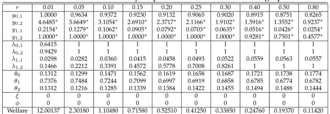
Examples in the first set (tables 1 and 2) are consistent with the optima having at most one nonbinding producer participation constraint, the one in meetings of producers with nothing and consumers with two units of money. In those meetings, although consumers transfer the same amount of money (except for r = 0.01) the optima presentsy0,1 < y0,2.
It raisesv2 −v1 and than relax producer participation constraint in (1, j)meetings,
par-ticularly in(1,1)meetings which permits a lower λ1,1 and, as consequence, a biggerθ1.
However, forrhigh enough producers with nothing are always restricted and the output
in those meetings does not depend on the consumer money.
The most common meeting in the first set occurs between people with one unit of money. For all discount rate in my examplesλ1,1is low, which has two effect: (a) a positive
effect on the extensive margin, because it raisesθ1and decreasesθ0 andθ2; (b) a negative
effect on the intensive margin, because producers are not willing to deliver a big output for a low probability a receive money. Although the output in those meeting is close to zero, the functional form of the utility function permit a reasonable gain from trade. For example if the output is1%ofy∗then the gain from trade is near50%ofh(y∗).
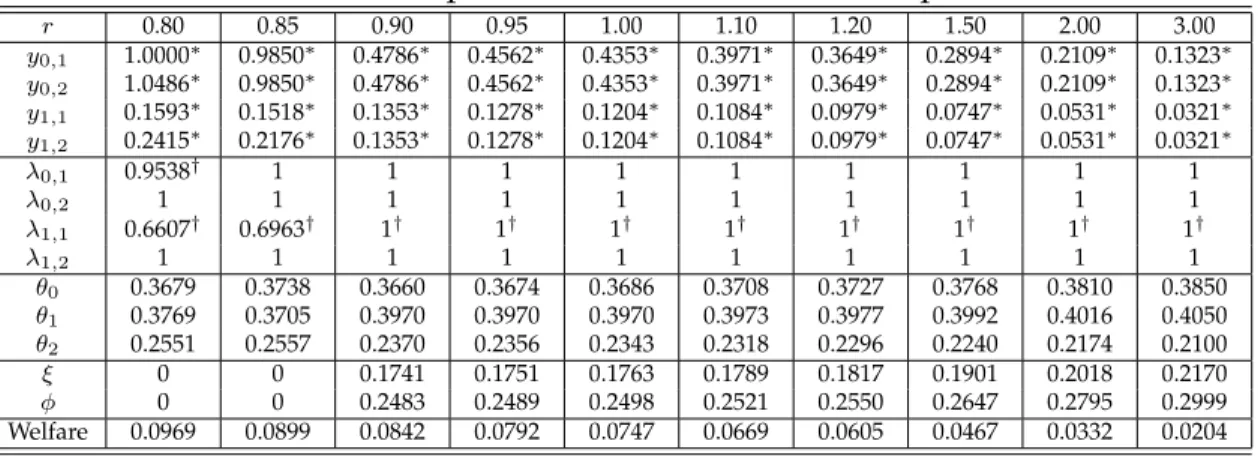
I report the examples for the second set in tables 3 and 4. The difference between this set of examples and the former is the addition of constraints in (16) to the planner
6For any positive probability of money transfer it is not stationary, and if there is no money transfers it
does not satisfies the of producers participation constraint.
7My optimum problem is included in the class of problems classified as ‘nonlinear programming
Table 1: Individual rationality implementable allocations - high patience
r 0.01 0.05 0.10 0.15 0.20 0.25 0.30 0.40 0.50 0.80
y0,1 1.0000 0.9634 0.9372 0.9230 0.9132 0.9065 0.9020 0.8915 0.8751 0.8265
y0,2 4.6485∗ 3.6649∗ 3.1054∗ 2.6910∗ 2.3717∗ 2.1166∗ 1.9102∗ 1.5916∗ 1.3552∗ 0.9237∗
y1,1 0.2154∗ 0.1279∗ 0.1062∗ 0.0905∗ 0.0792∗ 0.0703∗ 0.0635∗ 0.0516∗ 0.0426∗ 0.0254∗
y1,2 1.0000∗ 1.0000∗ 1.0000∗ 1.0000∗ 1.0000∗ 1.0000∗ 1.0000∗ 0.9281∗ 0.7501∗ 0.4577∗
λ0,1 0.6415 1 1 1 1 1 1 1 1 1
λ0,2 0.9429 1 1 1 1 1 1 1 1 1
λ1,1 0.0298 0.0282 0.0360 0.0415 0.0458 0.0493 0.0522 0.0559 0.0563 0.0557
λ1,2 0.1466 0.2212 0.3391 0.4572 0.5778 0.7008 0.8261 1 1 1
θ0 0.1312 0.1299 0.1471 0.1562 0.1619 0.1658 0.1687 0.1721 0.1738 0.1774
θ1 0.7376 0.7484 0.7244 0.7099 0.6997 0.6919 0.6858 0.6785 0.6774 0.6782
θ2 0.1312 0.1216 0.1285 0.1339 0.1384 0.1422 0.1455 0.1494 0.1488 0.1444
ξ 0 0 0 0 0 0 0 0 0 0
φ 0 0 0 0 0 0 0 0 0 0
Welfare 12.00137 2.30180 1.10480 0.71580 0.52510 0.41250 0.33850 0.24760 0.19370 0.11420
Table 2: Individual rationality implementable allocations - low patience
r 0.80 0.85 0.90 0.95 1.00 1.10 1.20 1.50 2.00 3.00
y0,1 0.8265 0.8190 0.8123 0.7890∗ 0.7449∗ 0.6686∗ 0.6050∗ 0.4674∗ 0.3328∗ 0.2049∗
y0,2 0.9237∗ 0.8758∗ 0.8324∗ 0.7890∗ 0.7449∗ 0.6686∗ 0.6050∗ 0.4674∗ 0.3328∗ 0.2049∗
y1,1 0.0254∗ 0.0239∗ 0.0224∗ 0.0209∗ 0.0194∗ 0.0179∗ 0.0157∗ 0.0127∗ 0.0089∗ 0.0052∗
y1,2 0.4577∗ 0.4278∗ 0.4016∗ 0.3777∗ 0.3567∗ 0.3208∗ 0.2916∗ 0.2266∗ 0.1623∗ 0.1009∗
λ0,1 1 1 1 1 1 1 1 1 1 1
λ0,2 1 1 1 1 1 1 1 1 1 1
λ1,1 0.0557 0.0554 0.0552 0.0551 0.0551 0.0551 0.0551 0.0549 0.0545 0.0538
λ1,2 1 1 1 1 1 1 1 1 1 1
θ0 0.1774 0.1779 0.1783 0.1790 0.1800 0.1816 0.1830 0.1857 0.1882 0.1902
θ1 0.6782 0.6786 0.6790 0.6791 0.6789 0.6786 0.6784 0.6783 0.6785 0.6792
θ2 0.1444 0.1435 0.1427 0.1419 0.1411 0.1398 0.1386 0.1360 0.1333 0.1306
ξ 0 0 0 0 0 0 0 0 0 0
φ 0 0 0 0 0 0 0 0 0 0
Welfare 0.11420 0.10650 0.09980 0.09380 0.08840 0.07920 0.07150 0.05500 0.03910 0.02390
problem. I attach daggers(†)to money transfers which correspond to binding core con-straints. Except for the(1,1)meetings, the core constraints are binding only if there is a
randomization over money transfers.
In general, the results have the same interpretation I gave to the first set, but there is a difference in the(1,1)meetings. Consumers spend more compared to the examples in the
first set, mainly if they are impatience. This is a direct consequence of the core constraint, because output is low then the marginal utility of consumption is high. Thus, a bigger monetary transfer is necessary to equalize the gains from consumer and producer. The consequence of the high spending in those meetings is a dispersion in the money distri-bution. If the lottery degenerates towards one unit, then the planner uses the monetary policy to improve the extensive margin in the economy.
Table 3: Core implementable allocations - high patience
r 0.01 0.05 0.10 0.15 0.20 0.25 0.30 0.40 0.50 0.80
y0,1 1.0000∗ 1.0000∗ 1.0000∗ 1.0000∗ 1.0000∗ 1.0000∗ 1.0000∗ 1.0000∗ 1.0000∗ 1.0000∗
y0,2 5.5064 3.7614 3.0748 2.7210 2.4951 2.3343 2.3291 2.1436∗ 1.7038∗ 1.0486∗
y1,1 0.2221∗ 0.2296∗ 0.2333∗ 0.2356∗ 0.2356∗ 0.2356∗ 0.2356∗ 0.2296∗ 0.2124∗ 0.1593∗
y1,2 1.0000∗ 1.0000∗ 1.0000∗ 1.0000∗ 1.0000∗ 1.0000∗ 0.8713∗ 0.6596∗ 0.4928∗ 0.2415∗
λ0,1 0.0438† 0.0915† 0.1474† 0.2022† 0.2565† 0.3107† 0.3610† 0.4667† 0.5872† 0.9538†
λ0,2 1 1 1 1 1 1 1 1 1 1
λ1,1 0.0325† 0.0682† 0.1102† 0.1514† 0.1921† 0.2326† 0.2704† 0.3476† 0.4306† 0.6607†
λ1,2 0.1460† 0.2972† 0.4717† 0.6435† 0.8155† 0.9888† 1 1 1 1
θ0 0.1460 0.1932 0.2244 0.2448 0.2600 0.2721 0.2824 0.3022 0.3232 0.3679
θ1 0.7342 0.6553 0.5992 0.5608 0.5314 0.5076 0.4888 0.4573 0.4302 0.3769
θ2 0.1198 0.1516 0.1764 0.1944 0.2086 0.2203 0.2288 0.2406 0.2466 0.2551
ξ 0 0 0 0 0 0 0 0 0 0
φ 0 0 0 0 0 0 0 0 0 0
Welfare 11.9599 2.2158 1.0455 0.6686 0.4853 0.3779 0.3075 0.2212 0.1704 0.0969
Table 4: Core implementable allocations - low patience
r 0.80 0.85 0.90 0.95 1.00 1.10 1.20 1.50 2.00 3.00
y0,1 1.0000∗ 0.9850∗ 0.4786∗ 0.4562∗ 0.4353∗ 0.3971∗ 0.3649∗ 0.2894∗ 0.2109∗ 0.1323∗
y0,2 1.0486∗ 0.9850∗ 0.4786∗ 0.4562∗ 0.4353∗ 0.3971∗ 0.3649∗ 0.2894∗ 0.2109∗ 0.1323∗
y1,1 0.1593∗ 0.1518∗ 0.1353∗ 0.1278∗ 0.1204∗ 0.1084∗ 0.0979∗ 0.0747∗ 0.0531∗ 0.0321∗
y1,2 0.2415∗ 0.2176∗ 0.1353∗ 0.1278∗ 0.1204∗ 0.1084∗ 0.0979∗ 0.0747∗ 0.0531∗ 0.0321∗
λ0,1 0.9538† 1 1 1 1 1 1 1 1 1
λ0,2 1 1 1 1 1 1 1 1 1 1
λ1,1 0.6607† 0.6963† 1† 1† 1† 1† 1† 1† 1† 1†
λ1,2 1 1 1 1 1 1 1 1 1 1
θ0 0.3679 0.3738 0.3660 0.3674 0.3686 0.3708 0.3727 0.3768 0.3810 0.3850
θ1 0.3769 0.3705 0.3970 0.3970 0.3970 0.3973 0.3977 0.3992 0.4016 0.4050
θ2 0.2551 0.2557 0.2370 0.2356 0.2343 0.2318 0.2296 0.2240 0.2174 0.2100
ξ 0 0 0.1741 0.1751 0.1763 0.1789 0.1817 0.1901 0.2018 0.2170
φ 0 0 0.2483 0.2489 0.2498 0.2521 0.2550 0.2647 0.2795 0.2999
Welfare 0.0969 0.0899 0.0842 0.0792 0.0747 0.0669 0.0605 0.0467 0.0332 0.0204
5.1 Discussion
The planner would implement an distribution of money close to θ∗ if she is restrict only
to individual incentives as suggested in tables 1 and 2. For all patient rate, she would choose θ1 > 0.67. To keep this stationary distribution of money, the planner limits the
spending in the meetings, specially in the (1,1) meetings because when the consumers
spend in those meetings the distribution of money becomes different fromθ∗. However,
people are anonymous in my economy and if there is a possibility of a better trade they will be free to deviate from planner’s allocation.
the spending in the(1,1)meetings generate a distribution of money less concentrated in
θ1. This make it difficult to people find good opportunities of trade, because some
po-tential producers have two units of money and some popo-tential consumers have nothing. This combination reduces the value of money (i.e., v1 and v2 fall), then the output in the
meetings become lower because producers are less willing to accept money.
An overview of my examples shows the existence of a conflict between private and collectiveinterests. Consumers want to increase their spending for more output while the
planner wants to implement a money distribution closer toθ∗asking people to spend less. This conflict becomes stronger when agents are impatient. More specifically, when β is
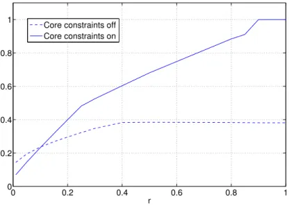
low producers have a tighter participation constraint, which reduces the output. Thus, consumers are more willing to spend, but the planner wants less spending to keep a good extensive margin, specially because the intensive margin is impaired. You can see the conflict grow by comparing the average spending with and without the core constraints in figure 1.8
0 0.2 0.4 0.6 0.8 1
0 0.2 0.4 0.6 0.8 1
r Core constraints off Core constraints on
Figure 1: Average spending
The planner uses the monetary policy, particularly inflation, as a response to the over-spending of the consumers. She avoid this instrument because the policy tightens the producers and, consequently, it implies a loss in the intensive margin. However, if the agents are impatient enough, the overspending makes a bad extensive margin, then the
8I computed the average spending, ¯λ, weighting the spending in each meeting by
the probability of that meeting compared to the frequency of productive meetings, i.e.,
¯
λ = (P1
i=0
P2
j=1θiθjλi,j)/(
P1
i=0
P2
j=1θiθj).
planner operates in the economy by altering the money distribution.
Despite Deviatov (2006) explicits that the absence of randomization in transfers of money is a characteristic of an allocation with an expansionary policy, he made a mis-take by reporting that the core restrictions are slack if there is no randomization.9 Let’s
compare my examples in tables 2 and 4, but forget the daggers in the last table for now. You can see a difference in the spending of consumers with one unit when they meet pro-ducers with one unit in those tables. While in table 2λ1,1 is close to zero for all discount
rate considered,λ1,1 = 1for almost all discount rate in table 4. Then, the core constraints
should be binding in those meetings, because they force the planner to choose a different allocation when they are imposed to the planner’s problem.
I think my results also qualify Deviatov and Wallace (2001) improvement in welfare from money creation. They use a notion of ex-post implementation which implies that any production must always be accompanied by a transfer of money and not just a posi-tive probability of money transfer. This requirement for trades generate an overspending. Thus, the planer choose a monetary policy to produce a better extensive margin for the economy.
6 Conclusion
The fundamental ideas behind this paper is to explore some consequences of the core constraints in a economy where people are anonymous. The examples in this paper show a conflict between private and collective interests. While the planner worry about the extensive and intensive margin effects of trades in a steady state, people want the exhaust the gains from trades immediately, i.e., once in a meeting, consumers prefer spend more for a better output now than take the risk of save money and wait for good meetings in the future. Thus, the core constraints can force the planner to choose allocations with a more disperse money distribution, mainly if people are impatient.
I admit that my model is abstract. For example, the only asset is indivisible money, people can not have more than two units or hide it and there is an absence of other insti-tutions that resemble modern economies. Nevertheless, my finds must hold for a higher upper bound to the money holdings for three reasons. First, the core constraints are im-posed to each meeting and the distribution of money are taken as given. Then, if people are anonymous, they would require to exhaust the gains from trade for any upper bound of the money distribution. Second, the monetary policy would keep the effect on the money distribution. Thus, it always possible to the planner to raise the fraction of agents
with money. Finally, even for a higher upper bound to the money holdings, there will be meetings with potential to disperse the distribution of money. Therefore, the conflict of interests must hold for a higher upper bound of money holdings.
A future research can explore some instruments and environment characteristics that can help the planner avoid core constraints. A direct method to avoid people from deviat-ing from a planner’s choice is add monitordeviat-ing in the economy in the sense of Cavalcanti and Wallace (1999). In meetings with monitored people the planner is not restricted to core constraints, because she can punish monitored people who deviate from her trade mechanism.10 I have a project in progress in which I extend my model here to incorporate
intermediation in the meetings. I think intermediation can work as a less extreme moni-toring if the intermediaries are persistent over the time and in an environment where the group of intermediaries is known, the planner can explore other mechanisms to improve the extensive margin.
10See Deviatov and Wallace (2013) and Wallace (2013) for some examples of inside and outside money
respectively. In both papers money holdings are limited to one unit and for all monitoring rate a positive inflation is part of the optima.
References
Byrd, R. H., J. Nocedal, and R. A. Waltz (2006). KNITRO: An integrated package for nonlinear optimization. InLarge Scale Nonlinear Optimization, 2006, pp. 35–59. Springer
Verlag.
Cavalcanti, R. d. O. and N. Wallace (1999). Inside and outside money as alternative media of exchange. Journal of Money, Credit and Banking 31(3), 443–57.
Deviatov, A. (2006). Money Creation in a Random Matching Model. Topics in Macroeco-nomics 6(3), 1–20.
Deviatov, A. and N. Wallace (2001). Another Example in which Lump-sum Money Cre-ation is Beneficial. Advances in Macroeconomics 1(1), 1–22.
Deviatov, A. and N. Wallace (2013). Optimal inflation in a model of inside money. Forth-coming in Review of Economic Dynamics.
Kehoe, T. J., D. K. Levine, and M. Woodford (1992). The optimum quantity of money revisited. In P. Dasgupta, D. Gale, O. Hart, and E. Maskin (Eds.),Economic Analysis of Markets and Games: Essays in Honor of Frank Hahn, pp. 501–526. Cambridge and London:
MIT Press.
Levine, D. K. (1991). Asset trading mechanisms and expansionary policy. Journal of Eco-nomic Theory 54(1), 148 – 164.
Li, V. E. (1995). The optimal taxation of fiat money in search equilibrium. International Economic Review 36(4), pp. 927–942.
Lucas, Robert E, J. (1980). Equilibrium in a pure currency economy.Economic Inquiry 18(2),
203–20.
Molico, M. (2006). The distribution of money and prices in search equilibrium. Interna-tional Economic Review 47(3), 701–722.
Scheinkman, J. A. and L. Weiss (1986). Borrowing constraints and aggregate economic activity. Econometrica 54(1), pp. 23–45.
Trejos, A. and R. Wright (1995). Search, Bargaining, Money, and Prices. Journal of Political Economy 103(1), 118–41.
Wallace, N. (2013). An attractive monetary model with surprising implications for optima: two examples. Mimeo.
Wallace, N. (2014). Optimal money creation in “pure currency” economies: a conjecture.
The Quarterly Journal of Economics 129(1), 259–274.
A Considerations on Deviatov (2006)
Deviatov (2006) built on the same environment used by Deviatov and Wallace (2001) (hereafter DW). Booth of them uses the mechanism design approach to characterize trades, but Deviatov examples are for ex-ante implementable allocation and DW work is built on ex-post implementable allocations. The latter notion of implementability requires that any output must always be accompanied by a transfer of money. Thus, the probability of a money transfer is also the probability of production in a meeting, then it has con-sequences for the expected utility. DW’s equation (4) (which I do not reproduce here) describes the vector of expected returns of one period.
I think Deviatov made a typographic error rewriting DW’s equation (4) for his ex-ante notion of implementability. Deviatov’s equation (3) can be written using my notation as:
q′ = 1 N
−θ1λ10,1c(y0,1)−θ2(λ10,2+λ 2
0,2)c(y0,2)
θ0λ10,1u(y0,1) +θ1λ11,1[u(y1,1)−c(y1,1)]−θ2λ11,2c(y1,2)
θ0(λ10,2+λ 2
0,2)u(y0,2) +θ1λ11,2u(y1,2)
. (18)
However the ex-ante notion of implementable allocations only requires a positive prob-ability of money transfer, because people commit with the lotteries. Then, the correct expected return of one period is:
q′ = 1 N
−θ1I{λ1
0,1}c(y0,1)−θ2I{λ 1 0,2+λ
2
0,2}c(y0,2)
θ0I{λ1
0,1}u(y0,1) +θ1I{λ 1
1,1}[u(y1,1)−c(y1,1)]−θ2I{λ 1
1,2}c(y1,2)
θ0I{λ1 0,2+λ
2
0,2}u(y0,2) +θ1I{λ 1
1,2}u(y1,2)
. (19) where
I{b} =
(
1 ifb >0
0 ifb = 0 .
probably miss-interpreted the multipliers of core constraints when agents are impatient. To conclude my note about about Deviatov’s paper, I notice a small difference between his examples and my numbers. Despite I share with him the same optimum problem (with identical functional forms), the examples diverge in the third or fourth decimal place for some of them. Probably, it is consequence of the numerical strategy adopted. While he built his own code (a generic algorithm) to solve the nonlinear programming problem, I use KNITRO, which is considered a good solver for this class of optimization problems. I think it is natural a small difference occurs in this case.