Vol. 5, No. 6, 2014
Forecasting Rainfall Time Series with stochastic
output approximated by neural networks Bayesian
approach
Cristian Rodriguez Rivero Department of Electronic Engineering
Universidad Nacional de Córdoba Córdoba, Argentina
Julian Antonio Pucheta Department of Electronic Engineering
Universidad Nacional de Córdoba Córdoba, Argentina
Abstract— The annual estimate of the availability of the amount of water for the agricultural sector has become a lifetime in places where rainfall is scarce, as is the case of northwestern Argentina. This work proposes to model and simulate monthly rainfall time series from one geographical location of Catamarca, Valle El Viejo Portezuelo. In this sense, the time series prediction is mathematical and computational modelling series provided by monthly cumulative rainfall, which has stochastic output approximated by neural networks Bayesian approach. We propose to use an algorithm based on artificial neural networks (ANNs) using the Bayesian inference. The result of the prediction consists of 20% of the provided data consisting of 2000 to 2010. A new analysis for modelling, simulation and computational prediction of cumulative rainfall from one geographical location is well presented. They are used as data information, only the historical time series of daily flows measured in mmH2O.
Preliminary results of the annual forecast in mmH2O with a
prediction horizon of one year and a half are presented, 18 months, respectively. The methodology employs artificial neural network based tools, statistical analysis and computer to complete the missing information and knowledge of the qualitative and quantitative behavior. They also show some preliminary results with different prediction horizons of the proposed filter and its comparison with the performance Gaussian process filter used in the literature.
Keywords—rainfall time series; stochastic method; bayesian approach; computational intelligence
I. INTRODUCTION
Climate variability in the semi-humid and arid parts of the northwestern part of Argentina poses a great risk to the people and resources of these regions [1] as the smallest fluctuations of weather parameters like precipitation not only damage the agriculture and economy of the region but disturb the overall water cycle [2].
The ANNs are mostly used as predictor filter with an unknown number of parameters performed by a lot of author, recently, such as in [3][4][5][6]. One famous black box model that forecast rainfall time series in recent decades is artificial neural network model. Artificial neural networks are free-intelligent dynamic systems models that are based on the experimental data, and the knowledge and covered law beyond data changes to network structure by trends on these data [7]. The difficulties in modeling such complex systems are
considerably reduced by the recent Artificial Intelligence tools like Artificial Neural Networks (ANNs); Genetic Algorithm (GA) [8] based evolutionary optimizer and Genetic Programming (GP).
In turn, this work propose to estimate water availability horizon useful for control problems in agricultural activities such as seedling growth and decision-making using some ANNs approaches presented in recent earlier works [9]. An ANNs filter is used and their parameters are set in function of the roughness of the time series. These are considered as random variables whose distribution is inferred by posterior probability from the data, in which is included as an additional parameter, the number of hidden neurons and modelling uncertainty [10].
The Bayesian approach permits propagation of uncertainty in quantities which are unknown to other assumptions in the model, which may be more generally valid or easier to guess in the problem. For neural networks, the Bayesian approach was pioneered in [11]-[12], and reviewed [13], [14] and [15]. The main difficulty in model building is controlling the complexity of the model. It is well known that the optimal number of degrees of freedom in the model depends on the number of training samples, amount of noise in the samples and the complexity of the underlying function being estimated.
The procedure of determining the prior density and likelihood functions associated with rainfall time series uncertainty is very complicated and there is a requirement to assume a linear and normal distribution within the framework of the proposed parameters. The problem of model selection is
often divided into discover an organization of a model’s
parameters that is well-matched such as the network topology, e.g. number of patterns, layers, hidden units per layer, that results in the best generalization performance. A common result is with too many free parameters tend to overfit the training data and, thus, show poor generalization performance.
useful inputs and “nuisance” inputs will contain too many free parameters and, thus, be prone to overfitting the training data leading to poor generalization.
II. DATA TREATMENT
A rainfall time series can be actually regarded as an integration of stochastic (or random) and deterministic components [16]. Once the stochastic (noise) component is appropriately eliminated, the deterministic component can then be easily modeled. Rainfall is an end product of a number of complex atmospheric processes which vary both in space and time; The data that is available to assist the definition of control variable for the process models, such as rainfall intensity, wind speed, and evaporation, etc. are linked in both the spatial and temporal dimensions; even if the rainfall can be described concisely and completely, the volume of calculations involved may be prohibitive; and the temporal and spatial resolution provided by this approach is not accurate enough for many hydrologic applications. A second approach to forecast rainfall makes use of nonparametric models based on statistics and/or machine learning.
The standard non-parametric approaches presented in this work by means of time-series analysis, is based on stochastic techniques that assume non-linear relationship among data that reproduce the rainfall time series only in statistical sense. Then, in principle, machine learning models, such as artificial neural networks, can improve the forecasting results obtained using models based on standard non-parametric approaches.
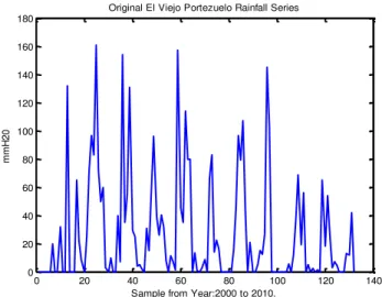
The rainfall dataset used is from Cuesta El Portezuelo located at Catamarca, province of Argentina (-28°28'11.26";-65°38'14.05") and the collection date is from year 2000 to 2010 shown in Fig.1.
Fig. 1. Original Rainfall times series from El Viejo Portezuelo, Catamarca, Argentina.
III. METHODOLOGY AND BAYESIAN APPROACH When a time series is being analyzed, it is important to make use of the simplest possible models. Specifically, the number of unknown parameters must be kept at a minimum.
For forecasting problems, Bayesian analysis generates point and interval forecasts by combining all the information and sources of uncertainty into a predictive distribution for the future values. It does so with a function that measures the loss to the forecaster that will result from a particular choice of forecasts.
The gamma distributions have been chosen for this purpose. When a Bayesian analysis is conducted, inferences about the unknown parameters are derived from the posterior distribution. This is a probability model which describes the knowledge gained after observing a set of data. The application of the regression problem involving the correspond neural network function y(x,w) and the data set consisting of N pairs, input vector lx and targets tn(n=1,….,N).
Assuming Gaussian noise on the target, the likelihood function takes the form:
, ) ; ( 2 exp 2
) , / (
1
2 2
/
N n
n n N
t w x y M
w D
P
(8)
where
is a hyper-parameter representing the inverse of the noise variance. We consider in this work a single hidden layer of ‘tanh’ units and a linear outputs units.To complete the Bayesian approach for this work, prior information for the network is required. It is proposed to use, analogous to penalties terms, the following equation
,2 exp 2
)
( 2
2 2
/ 2
w w w
w
P N (9)
assuming that the expected scale of the weights is given by w set by hand. This was carried out considering that the network function f(xn+1,w) is approximately linear with respect to w in the vicinity of this mode, in fact, the predictive distribution for yn+1 will be another multivariate Gaussian.
IV. PROPOSED APPROACH FOR TUNING THE NEURAL NETWORKS BY BAYESIAN APPROACH
In the block diagram of the nonlinear prediction scheme based on a ANN filter is shown. Here, a prediction device [17]-[18] is designed such that starting from a given sequence {xn}
at time n corresponding to a time series it can be obtained the best prediction {xe} for the following sequence of 18 values.
Hence, it is proposed a predictor filter with an input vector lx, which is obtained by applying the delay operator, Z-1, to the
sequence {xn}. Then, the filter output will generate xe as the
next value, that will be equal to the present value xn. So, the
prediction error at time k can be evaluated as:
e
k xn
k xe
k (6)which is used for the learning rule to adjust the NN weights.
0 20 40 60 80 100 120 140 0
20 40 60 80 100 120 140 160 180
Original El Viejo Portezuelo Rainfall Series
Sample from Year:2000 to 2010.
m
m
H
2
Vol. 5, No. 6, 2014
Fig. 2. Block diagram of the nonlinear prediction.
The coefficients of the nonlinear ANNs filter are adjusted on-line in the learning process, by considering an online heuristic criterion that modifies at each pass of the time series the number of patterns, the number of iterations and the length
in function of the Hurst’s value H calculated from the time series taking into account the Bayesian inference and stochastic dependence of the output values.
A. Bayesian model
When a rainfall series is being analyzed, it is important to make use of the simplest possible models. Specifically, the number of unknown parameters must be kept at a minimum. For forecasting problems, Bayesian analysis generates point and interval forecasts by combining all the information and sources of uncertainty into a predictive distribution for the future values. It does so with a function that measures the loss to the forecaster that will result from a particular choice of forecasts.
The gamma distributions have been chosen for this purpose. When a Bayesian analysis is conducted, inferences about the unknown parameters are derived from the posterior distribution. This is a probability model which describes the knowledge gained after observing a set of data. The application of the regression problem involving the correspond neural network function y(x,w) and the data set consisting of N pairs, input vector lx and targets tn(n=1,….,N)
Assuming Gaussian noise on the target, the likelihood function takes the form:
, ) ; ( 2 exp 2
) , / (
1
2 2
/
N n
n n N
t w x y M
w D
P
(7)
where
is a hyper-parameter representing the inverse of the noise variance. We consider in this work a single hiddenlayer of ‘tanh’ units and a linear outputs units. To complete the Bayesian approach for this work, prior information for the network is required. It is proposed to use, analogous to penalties terms, the following equation,
, 2 exp 2
)
( 2
2 2
/ 2
w w w
w
P N
(8)
assuming that the expected scale of the weights is given by w set by hand. This was carried out considering that the network function f(xn+1,w) is approximately linear with respect to w in the vicinity of this mode, in fact, the predictive distribution for yn+1 will be another multivariate Gaussian.
The computation test results were made on rainfall time series, which consist of 132 data. The Monte Carlo method was employed to forecast the next 18 values with an associated variance. Here it was performed an ensemble of 500 trials with a fractional Gaussian noise sequence of zero mean and variance of 0.11. The fractional noise was generated by the Hosking method [19] with the H parameter estimated from the data time series. The following figures yield the results of the mean and the variance of 500 trials of the forecasted 18 values. Such outcomes for one (30%) and two (69%) sigma are shown in Fig. 6, Fig. 7, Fig. 8, Fig. 10, and Fig. 11. The obtained time series has a mean value, denoted at the foot of the figure by
“Forecasted Mean”, whereas the “Real Mean” although it is not
available at time 114. This procedure is repeated 500 times for each time series.
The assessment of the experimental results has been obtained by comparing the performance of the proposed filter against the Gaussian process based filter. The evolution of the SMAPE index for a neural network bayesian approach filter, which uses a learning algorithm and the GP filter has the same initial parameters in each algorithm, although such parameters
and filter’s structure are changed by the proposed approach, not
is the case of the GP filter. In the proposed filter, the coefficients and the structure of the filter are tuned by considering their stochastic dependency. It can be noted that in each one of Fig. 3 to Fig. 6.
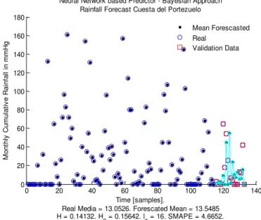
Fig. 3. Cuesta El Portezuelo Rainfall time series neural network Bayesian approach.
0 20 40 60 80 100 120 140
0 20 40 60 80 100 120 140 160 180
Neural Network based Predictor - Bayesian Approach Rainfall Forecast Cuesta del Portezuelo
Time [samples].
Real Media = 13.0526. Forescated Mean = 13.5485 H = 0.14132. He = 0.15642. lx = 16. SMAPE = 4.6652.
M
o
n
th
ly
C
u
m
u
la
ti
v
e
R
a
in
fa
ll
in
m
m
H
g
Mean Forescasted Real
Validation Data
Estimation of prediction error
Z-1 I Error-correction signal
One-step prediction
Fig. 4. Cuesta El Portezuelo Rainfall time series Bayesian approach forecast horizon.
Fig. 5. Cuesta El Portezuelo Rainfall time series stochastic output with zero mean and 0.11 variance.
Fig. 6. Cuesta El Portezuelo Rainfall time series stochastic forecast horizon.
Fig. 7. Cuesta El Portezuelo Rainfall time series Gaussian process filter.
Fig. 8. Cuesta El Portezuelo Rainfall time series Gaussian process filter forecast horizon
.
Fig. 9. Cuesta El Portezuelo Rainfall time series stochastic Gaussian Process
114 116 118 120 122 124 126 128 130 132 134 0 10 20 30 40 50 60 70
Horizon of the Forecast Rainfall Forecast Cuesta del Portezuelo
Time [samples].
Real Media = 13.0526. Forescated Mean = 13.5485 H = 0.14132. SMAPE = 4.6652.
M o n th ly C u m u la ti v e R a in fa ll in m m H g Mean Forescasted Data Validation Data
0 20 40 60 80 100 120 140 0 20 40 60 80 100 120 140 160 180 Time [samples].
Real Media = 13.0526. Forescated Mean = 17.6546. H = 0.14132. He = 0.12827. lx = 8. SMAPE = 31.2089.
M o n th ly C u m u la ti v e R a in fa ll in m m H g
Stochastic output approximate by neural networks Bayesian approach Rainfall Forecast Cuesta del Portezuelo
Borders Data Validation data
114 116 118 120 122 124 126 128 130 132 0 10 20 30 40 50 60 70 80 90 Time [samples].
Real Media = 13.0526. Forescated Mean = 17.6546. H = 0.14132 SMAPE = 31.2089.
M o n th ly C u m u la ti v e R a in fa ll in m m H g
Horizon of the Rainfall Forecast Cuesta El Portezuelo
Borders Data
0 20 40 60 80 100 120 140 0 20 40 60 80 100 120 140 160 180
Gaussian Process Filter Predictor Rainfall Cuesta el Portezuelo
Time [samples].
Real Media = 13.0526. Forescated Mean = 15.7866. SMAPE = 27.9517.
M o n th ly C u m u la ti v e R a in fa ll in m m H g Mean Forescasted Real Validation Data
114 116 118 120 122 124 126 128 130 132 0 10 20 30 40 50 60 70
Horizon of the Forecast Rainfall Cuesta el Portezuelo
M o n th ly C u m u la ti v e R a in fa ll in m m H g Time [samples].
Real Media = 13.0526. Forescated Mean = 15.7866. SMAPE = 27.9517.
0 20 40 60 80 100 120 140 0 20 40 60 80 100 120 140 160 180 Time [samples].
Real Media = 13.0526. Forescated Mean = 18.1989. SMAPE = 35.9921.
Stochastic output approximate by Gaussian Process Predictor Filter
Vol. 5, No. 6, 2014
Fig. 10.Cuesta El Portezuelo Rainfall time series stochastic forecast horizon. The measure of forecast performance is measured by the Symmetric Mean Absolute Percent Error (SMAPE) proposed in the most of metric evaluation, defined by
(9)
where t is the observation time, n is the size of the test set, s is each time series, Xt and Ft are the actual and the forecasted
time series values at time t respectively. The SMAPE of each series s calculates the symmetric absolute error in percent between the actual Xt and its corresponding forecast value Ft,
across all observations t of the test set of size n for each time series s.
In each figure are detailed the testing and the computing data, where the testing are labelled “Validation data” and had not been used in the computation of the predictor filter.
In table I, the better performance is shown by the stochastic NN Bayesian approach where the index is set to 4.66 and 31.20. By means of this assessment, the approach can be applied for a class of high roughness rainfall time series, in this case measured by the Hurst parameter [20] to Cuesta El Portezuelo series, H=0.14.
TABLE I. FIGURES OBTAINED BY THE PROPOSED APPROACH FOR EACH PREDICTOR FILTER
Filters for Rainfall time
series Real Mean
Mean
Forecasted SMAPE
NN Bayesian approach 13.05 13.56 4.66 Gaussian Process 13.05 15.78 27.95 Stochastic NN Bayesian
approach 13.05 17.65 31.20 Stochastic Gaussian
Process 13.05 18.19 35.99
V. CONCLUSIONS
In this article, forecasting rainfall time-series with stochastic output approximated by neural networks Bayesian approach has been presented. In the first case, an ANNs algorithm based on Bayesian inference to model neural networks parameters were detailed. The learning rule proposed
to adjust the ANN’s coefficients was based on the Levenberg -Marquardt method.
Furthermore, the rainfall series were related with the long or short term stochastic dependence of the time series assessed by the Hurst parameter H, then the stochastic approximation to forecast the next 18 month were implemented. Its main contribution lies in generating stochastic rainfall time series forecast from monthly cumulative rainfall data, which allows adjusting the filter parameters for each algorithm and then averaged over all the outputs. The roughness of the resulting forecasted time series was again evaluated by the Hurst parameter H in the Bayesian approach.
The main results show a good performance of the predictor system based on stochastic neural network Bayesian approach, applied to time series obtained from a geographical point when the observations are taken from a single point due to similar roughness for both, the original and the forecasted time series, respectively.
These results encouraged us to continue working on new machine learning algorithms using novel forecasting methods.
ACKNOWLEDGMENT
This work was supported by Universidad Nacional de Córdoba (UNC), FONCYT-PDFT PRH N°3 (UNC Program RRHH03), SECYT-UNC, Institute of Automatic (INAUT) - Universidad Nacional de San Juan and National Agency for Scientific and Technological Promotion (ANPCyT).
REFERENCES
[1] Center for Studies of Variability and Climate Change (CEVARCAM) - Facultad de Ingeniería y Ciencias Hídricas (FICH), Universidad Nacional del Litoral (UNL).
[2] Magrin, G.raciela, Maria Travasso, Raul Diaz, and Rafael Rodriguez. 1997. “Vulnerability of the agricultural systems of Argentina to climate change”, Climate Research 9: 31-36.
[3] Menhaj, M.B., 2012. Artificial Neural Networks. Amirkabir University of Technology.
[4] Cristian M. Rodríguez Rivero, Julián A. Pucheta, Martín R. Herrera, Victor Sauchelli, Sergio Laboret. Time Series Forecasting Using Bayesian Method: Application to Cumulative Rainfall, (Pronóstico de Series Temporales usando inferencia Bayesiana: aplicación a series de lluvia de agua acumulada). ISSN 1548-0992. Pp. 359 364. IEEE LATIN AMERICA TRANSACTIONS, VOL. 11, NO. 1, FEB. 2013. http://www.ewh.ieee.org/reg/9/etrans/ieee/issues/vol11/vol11issue1Feb. 2013/11TLA1_62RodriguezRivero.pdf
[5] Julián A. Pucheta , Cristian M. Rodríguez Rivero , Martín R. Herrera, Carlos A. Salas, H. Victor Sauchelli. “Rainfall Forecasting Using Sub sampling Nonparametric Methods” (“Pronóstico de lluvia usando métodos no paramétricos con submestreo”). ISSN 1548-0992. Pp. 346-350. IEEE LATIN AMERICA TRANSACTIONS, VOL. 11, NO. 1, FEB.2013.
http://www.ewh.ieee.org/reg/9/etrans/ieee/issues/vol11/vol11issue1Feb. 2013/11TLA1_110Pucheta.pdf
114 116 118 120 122 124 126 128 130 132
0 20 40 60 80 100 120
Time [samples].
Real Media = 13.0526. Forescated Mean = 18.1989. SMAPE = 35.9921.
M
o
n
th
ly
C
u
m
u
la
ti
v
e
R
a
in
fa
ll
i
n
m
m
H
g
Horizon of the Rainfall Forecast Cuesta El Portezuelo
[6] C. Rodriguez Rivero, J. Pucheta, H. Patiño, J. Baumgartner, S. Laboret and V. Sauchelli. “Analysis of a Gaussian Process and Feed-Forward Neural Networks based Filter for Forecasting Short Rainfall Time Series”. 2013 International Joint Conference on Neural Networks, Texas, 4 al 9 de Agosto de 2013, USA. Print Edition: IEEE Catalog Number: CENSUS-ART, ISBN: 978-1-4673-6129-3, ISSN: 2161-4407, CD Edition: IEEE Catalog Number: CFPlSUS-CDR, ISBN: 978-1-4673-6128-6. 2013.
[7] Salas, J.D., Delleur, J.W., Yevjevich, V., Lane, W.L. (Eds.), 1985. Applied Modeling of Hydrologic Time Series. Water Resources Publications, Littleton, Colorado.
[8] Baumgartner, J.; Rodríguez Rivero, C. y Pucheta, J. (2011) “Pronóstico de lluvia en un punto desde diversos puntos geográficos de observación mediante procesos gaussianos.” XXIII Congreso Nacional del Agua – CONAGUA, 22 al 25 de Junio de 2011, Resistencia, Chaco, Argentina, ISSN 1853-7685.
[9] J. Pucheta, M., C. Rodríguez Rivero, M. Herrera, C. Salas, D. Patiño and B. Kuchen. A Feed-forward Neural Networks-Based Nonlinear Autoregressive Model for Forecasting Time Series. Revista Computación y Sistemas, Centro de Investigación en Computación-IPN, México D.F., México, Computación y Sistemas Vol. 14 No. 4, 2011, pp
423-435, ISSN 1405-5546.
http://www.cic.ipn.mx/sitioCIC/images/revista/vol14-4/art07.pdf [10] C. Rivero Rodríguez, J. Pucheta, J. Baumgartner, M. Herrera, H.D.
Patiño and V. Sauchelli, Bayesian modeling of a nonlinear autoregressive filter based on neural networks for monthly cumulative rainfall time series forecasting , anales del Congreso CONAGUA (Congreso Nacional del Agua), ISSN 1853-7685, Chaco, Argentina, realizado del 22 al 25 de Junio, 2011. [11] Buntine, W. L., & Weigend, A. S. (1991). Bayesian back-propagation. Complex Systems, 05(6), 603.
[12] D.J.C. MacKay, A practical Bayesian framework for backpropagation networks, Neural Comput. 4 (1992) 448}472.
[13] Bishop, C. (2006). Pattern Recognition and Machine Learning. Boston: Springer.
[14] MacKay, D. J. C. (1995). Probable networks and plausible predictions - a review of practical Bayesian methods for supervised neural networks. Network: Computation in Neural Systems, 6 (3), 469-505.
[15] R.M. Neal, in: Bayesian learning for neural networks, Lecture Notes in Statistics, Vol. 118, Springer, New York, 1996.
[16] Pucheta, J., Patino, D. and Kuchen, B. “A Statistically Dependent Approach For The Monthly Rainfall Forecast from One Point Observations”. In IFIP International Federation for Information Processing Volume 294, Computer and Computing Technologies in Agriculture II, Volume 2, eds. D. Li, Z. Chunjiang, (Boston: Springer), pp. 787–798. (2009).
[17] Pucheta, J., Patiño, H.D., Kuchen, B. (2007). Neural Networks-Based Time Series Prediction Using Long and Short Term Dependence in the Learning Process. In proc. of the 2007 International Symposium on Forecasting, New York, USA.
[18] Pucheta, J., Rodriguez Rivero, C., Herrera, M., Sauchelli, V. and J. Baumgartner . “Time Series Forecasting using Kernel and Feed-Forward Neural”. XIV Reunión de Trabajo en Procesamiento de la Información y Control RPIC 2011, 16 al 18 de Noviembre de 2011 Oro Verde, Entre Ríos, Argentina. (2011).
[19] Dieker, T. (2004). Simulation of fractional Brownian motion. The Netherlands MSc theses, University of Twente Amsterdam.