Artificial Neural Networks versus Box-Jenkins Methodology in Tourism Demand Analysis

Congress Thematic Topics: Spatial econometrics

Artificial Neural Networks versus Box-Jenkins Methodology in

Tourism Demand Analysis

Fernandes, Paula (pof@ipb.pt) Department of Economics and Management School of Technology and Management (ESTiG)

Polytechnic Institute of Bragança (IPB) Apartado 134, 5301-857 Bragança, Portugal Tel: +351273313050, Fax: +351273313051

Teixeira, João (joaopt@ipb.pt) Department of Electrical Engineering School of Technology and Management (ESTiG) Polytechnic Institute of Bragança (IPB) Apartado 134, 5301-857 Bragança, Portugal Tel: +351273313050, Fax: +351273313051

Ferreira, João (jjmf@ubi.pt) Department of Management and Economics

University of Beira Interior (UBI) Pólo IV - Edifício Ernesto Cruz, 6200-209 Covilhã, Portugal Tel: +351275319600, Fax: +351275319601

Azevedo, Susana (sazevedo@ubi.pt) Department of Management and Economics

University of Beira Interior (UBI) Pólo IV - Edifício Ernesto Cruz, 6200-209 Covilhã, Portugal Tel: +351275319600, Fax: +351275319601

ABSTRACT

Several empirical studies in the tourism area have been performed and published during the last

decades. The researchers are unanimous upon considering that in the planning process,

decision-making and control of the tourism sector, the forecast of the tourism demand assumes an important

role.

Nowadays, there is a great variety of methods for forecasting that have been developed and which

can be applied in a set of situations presenting different characteristics and methodologies, going from

simple approaches to more complex ones.

In this context, the present study aims to explore and to evidence the usefulness of the Artificial Neural

Networks methodology (ANN), in the analysis of the tourism demand, as an alternative to the

Box-Jenkins methodology. ANN has been under attention in the area of business and economics

since, in this field, it presents this methodology as a valid alternative to classical methods of

forecasting allowing its application for problems in which the traditional ones would be difficult to use

ability for improving time-series forecasts by mining additional information, diminishing their

dimensionality, and reducing their complexity. In this way, for each methodology treatment, analysis

and modeling of the tourism time-series: “Nights Spent in Hotel Accommodation per Month” registered

between January 1987 and December 2006, was carried out since is one of the variables that better

explains the effective tourism demand. The study was performed for the North and Center regions of

Portugal. Considering the results, and according to the Criteria of MAPE for model evaluation in Lewis

(1982), the ANN model presented an acceptable goodness of fit and good statistical properties and is,

therefore, adequate for modelling and prediction of the reference time series, when compared to the

results obtained by the methodology of Box-Jenkins.

Keywords: Artificial Neural Networks; Backpropagation; Box-Jenkins Methodology; Time Series Forecasting; Tourism Demand.

JEL: C01; C02; C22; C45; L83.

1. Introduction

Countless empirical studies have been undertaken and published in the field of tourism in recent

years, and they are unanimous in considering that the forecasting of tourism demand has an important

role to play in the planning, decision-making and control of the tourism sector (Witt & Witt, 1995;

Wong, 2002; Fernandes, 2005; Yu & Schwartz, 2006).

Currently available in the field of forecasting are a wide range of methods that have emerged in

response to the most varied situations, displaying different characteristics and methodologies and

ranging from the simplest to the most complex approaches. The Box-Jenkins forecasting models

belong to the family of algebraic models known as ARIMA models, which make it possible to make

forecasts based on a given stationary time series. The methodology considers that a real time series

amounts to a probable realization of a certain stochastic process. The aim of the analysis is to identify

the model that best depicts the underlying unknown stochastic process and which also provides a

good representation of its realisation, i.e. of the real time series. Another methodology that has had

countless applications in the most diverse areas of knowledge and has been used in the field of

forecasting as an alternative to the classical models involves the use of models based on artificial

neural networks. These non-linear models first appeared as an attempt to reproduce the functioning of

the human brain, with the complex system of biological neurones being their main source of

inspiration.

The aims of this current research are to investigate and highlight the usefulness of the Artificial Neural

Networks methodology as an alternative to the Box-Jenkins methodology in analysing tourism

demand, and to assess the performance and competitiveness of tourist destinations by main supply

markets. The first methodology has aroused great interest in the field of economic and business

alternative to classical forecasting methods, providing a response to situations that would be difficult to

treat through classical methods (Thawornwong & Enke, 2004). Hill et al. (1996) and Hansen et al.

(1999) state that ANN demonstrate a capacity for improving time series forecasting through the

analysis of additional information, reducing its size and lessening its complexity. To this end, each of

the above-mentioned methodologies is centred on the treatment, analysis and modelling of the

tourism time series: “Nights Spent in Hotel Accommodation per Month”. Due to its characteristics, the

series Nights Spent in Hotel Accommodation per Month is considered a significant indicator of tourist

activity, since it provides information about the number of visitors that have taken advantage of tourist

facilities. The study was undertaken for two regions of Portugal: the North and Centre regions. Thus,

the analysis undertaken in this research will be based on a study of the Nights Spent per Month

recorded in the North region [DRN] and the Nights Spent per Month recorded in the Centre region

[DRC]. The data observed cover the period between January 1987 and December 2006,

corresponding to 240 monthly observations over the 20-year period.

The current research is structured as follows: after the introduction, the methodologies that are used,

namely the artificial neural networks and the Box-Jenkins methodology, will be presented in the

second section. Next, the time series “Nights spent per Month by tourists” is presented and analysed

for the regions under study, with models being built and tourism demand being forecast for the years

2005 and 2006. In section three, an assessment will be made of the competitiveness between the

tourist destinations analysed. Finally, in section four, the conclusions will be presented and possible

future developments will be suggested.

2. Artificial Neural Networks versus the Box-Jenkins Methodology 2.1. Methodologies Used

The methodology proposed by Box and Jenkins, in 1970, makes it possible to undertake an analysis

of the behaviour of time series, based on a joint double study: on the one hand, there is an

autoregressive component that is established in accordance with the previous statistical history of the

variables considered and, on the other hand, there is a treatment of the random or stochastic factors,

specified through the use of moving averages. Due to their delineation scheme and operative

resolution, these models allow for the incorporation of seasonal analyses and the isolation of the trend

component, also making it possible to go deeper into the interrelations between these components,

which are integrated into the evolution of the series under study (Parra & Domingo, 1987; Chu, 1998).

The models introduced by Box and Jenkins exclusively describe stationary series, or, in other words,

series with constant mean and variance over time and autocovariance dependent only on the extent of

the phase lag between the variables, so that one should begin by checking or provoking the

stationarity of the series (Pulido, 1989). These are the so-called ARIMA (Autoregressive Integrated

Moving Average) models, which are quite suitable for short-term forecasting and for the case of series

Thus, in order to use the Box-Jenkins methodology, one must first identify the series and remove the

non-stationarity, so that one or more transformations need to be made to the values of the series in

order to obtain another stationary series (with transformed original values). Although they preserve the

general structure of the series, such transformations have considerable effects on the set of data,

making its actual study easier, altering its scale (and possibly diminishing its amplitude), reducing

asymmetries, eliminating possible outliers, lessening residuals and finally achieving the aims in

question: stabilising variances and linearising trends (Otero, 1993; Fernandes & Cepeda, 2000). After

the series has been identified, its parameters need to be estimated and then an assessment must be

made of the adjustment. If necessary, a new model will have to be found that better describes the

phenomenon in question. Finally, there comes the forecasting phase.

In this sense, the ARIMA model (p,d,q), in which p corresponds to the order of the Autoregressive

process (AR), d is the number of differences or integrations, and q corresponds to the order of the

Moving Averages process (MA), is represented by the following expression (Murteira et al., 1993; Zou

& Yang, 2004):

(

1

1

)

(

1

)

(

1

1

)

d

p q

p t q t

B

B

B

Y

B

B

e

φ

φ

θ

θ

−

−

−

−

=

−

−

−

[1]

or also, in a more summarised form, by:

( )

d

( )

p

B

Y

t q

B e

t

φ

∇

=

θ

[2]

ARIMA models are normally used with quarterly, monthly or even weekly, daily or hourly data, or, in

other words, in a context of short-term forecasting. For such purposes, ARIMA models are used to

capture seasonal behaviour, in a manner that is identical to the treatment of the regular (or

non-seasonal) component of the series. In such applications, it is not customary to work with just one

ARIMA model (p,d,q), but with the product of the models: ARIMA

₍

p,d,q P,D,Q

₎₍

₎

sin which the first part corresponds to the regular part and the second to the seasonal part, corresponding to the following

expression (Murteira et al., 1993; Zou & Yang, 2004):

( )

( )

S

(

1

)

d

(

1

S

)

D

( )

( )

S

p

B

P

B

B

B

Y

t q

B

Q

B

e

t

φ

Φ

−

−

=

θ

Θ

[3]

The forecasts made with the ARIMA model, based on historical data, are given by the forecasting

function:

( )

{

}

*

1 2

/

,

,

,

t t m t t t

Y

m

= Ε

Y

₊

Y Y

₋

Y

₋ [4]

Another methodology that has been afforded some attention by the scientific community in recent

years, showing some advances in the knowledge of management sciences, is based on the use of

artificial neural networks (ANN). ANN are models that are frequently found within the broad field of

knowledge relating to artificial intelligence. They are based on mathematical models with an

architecture that is similar to that of the human brain. A neural network is composed of a set of

interconnected artificial neurons, nodes, perceptrons or a group of processing units, which process

known as synapses. The functions most frequently used are the linear and the sigmoidal functions -

the logistic and hyperbolic tangent functions - (Rodrigues, 2000; Fernandes, 2005). It should also be

mentioned that the neurons of a network are structured in distinct layers (better known as the input

layer, the intermediate or hidden layer and the output layer), with the ones most commonly used for

the forecasting of time series being the multi-layers or MLP1 (Bishop, 1995), so that a neuron from one

layer is connected to the neurons of the next layer to which it can send information, Figure 1,

(Fernandes, 2005). Depending on the way in which they are linked between the different layers,

networks can be classified as either feedback networks2 or feedforward networks3.

Figure 1. Structure of a Feedforward Artificial Neural Network (Adapted from Haykin, 1999:13).

The specification of the neural network also includes an error function and an algorithm to determine

the value of the parameters that minimise the error function. In this way, there are two central

concepts: the physical part of the network, or, in other words, its architecture, and the algorithmic

procedure that determines its functioning, or, in other words, the way in which the network changes

according to the data provided by the environment (Haykin, 1999).

It is also important to mention that for the ANN to learn with experience they have to be submitted to a

process known as training, for which there are different training algorithms. One of the most frequently

used algorithms in the forecasting of time series is the backpropagation4 algorithm or its variants,

which are distributed into two classes: (i) supervised and (ii) unsupervised (Haykin, 1999). For the first

case, during the training process, there is a “teacher” that provides a set of training cases, and a

training case consists of an input vector

X

and the corresponding output vector

Y

. Learning involves

the minimisation of the output error, which is achieved by adjusting the weights of the connections

according to a certain rule. In the second case, there is a set of inputs, so that the training algorithm

tries to group the data according to patterns presented by these, thus following a rule of

self-organisation (Haykin, 1999; Fernandes, 2005).

1

Multilayer Perceptron.

2

The connections allow information to return to places through which it has already passed and also allow for (lateral) inter-layer connections (Fernandes, 2005).

3

Information flows in one direction from one layer to another, from the input layer to the hidden layer and then to the output layer (Fernandes, 2005).

4

This algorithm seeks the minimum error function in the demand space of the weights of the connections between the neurones, being based on gradient descent methods. The combination of weights that minimises the error function is considered to be the solution for the learning problem. The description of the algorithm can be analysed in Rumelhart and McClelland (1986) and Haykin (1999).

Input Layer

Hidden Layer

Yt

X1

Xn

0 100,000 200,000 300,000 400,000 500,000 600,000 J a n -8 7 J a n -8 8 J a n -8 9 J a n -9 0 J a n -9 1 J a n -9 2 J a n -9 3 J a n -9 4 J a n -9 5 J a n -9 6 J a n -9 7 J a n -9 8 J a n -9 9 J a n -0 0 J a n -0 1 J a n -0 2 J a n -0 3 J a n -0 4 J a n -0 5 J a n -0 6 M onths N .º o f O v e rn ig h t - N o rt h r e g io n 0 100,000 200,000 300,000 400,000 500,000 600,000 J a n -8 7 J a n -8 8 J a n -8 9 J a n -9 0 J a n -9 1 J a n -9 2 J a n -9 3 J a n -9 4 J a n -9 5 J a n -9 6 J a n -9 7 J a n -9 8 J a n -9 9 J a n -0 0 J a n -0 1 J a n -0 2 J a n -0 3 J a n -0 4 J a n -0 5 J a n -0 6 M onths N .º o f O v e rn ig h t - C e n tr e r e g io n

In short, a value produced by a feedforward network, with a hidden layer, can be expressed as follows

(Fernandes & Teixeira, 2007):

2,1 1,

1 1

n m

t j ij t i j

j i

Y

b

α

f

β

y

−

b

= =

=

+

+

[5]

where,

m

, number of nodes in the input layer;

n

, number of nodes in the hidden layer;

f

, sigmoidal activation function;

{

α

_j

,

j

=

0,1,

,

n

}

, vector of weights that connects the nodes of the hidden layer to those of the output layer;

{

β

_ij

,

i

=

0,1,

,

m j

;

=

1, 2,

,

n

}

, weights that connect the nodes of the input layer to those of the

hidden layer;

2,1

b

and

b

_1,j, indicate the weights of the independent terms (bias) associated with each node of

the output layer and the hidden layer, respectively.

The equation also indicates the use of a linear activation function in the output layer.

2.2. Presentation and Analysis of the Time Series Behaviour

The series Nights Spent in Hotel Accommodation per Month is considered a significant indicator of

tourist activity, since it provides information about the number of visitors that have taken advantage of

tourist facilities, in this case in the North and Centre regions of Portugal.

Thus, the analysis undertaken in this research will be based on a study of the series Nights Spent per

Month recorded in the North region [DRN] and Nights Spent per Month recorded in the Centre region

[DRC]. The data observed cover the period between January 1987 and December 2006,

corresponding to 240 monthly observations over the 20-year period (see Appendix A, Tables A.1 and

A.2). The values of the series were provided by the Portuguese National Statistical Office (INE).

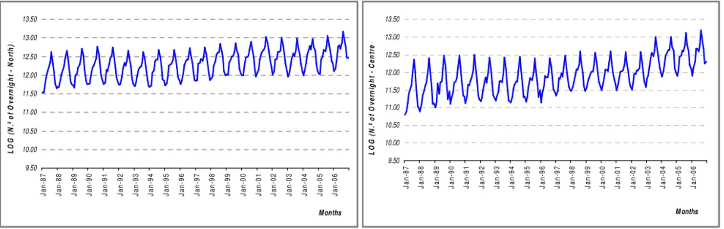
9.50 10.00 10.50 11.00 11.50 12.00 12.50 13.00 13.50 J a n -8 7 J a n -8 8 J a n -8 9 J a n -9 0 J a n -9 1 J a n -9 2 J a n -9 3 J a n -9 4 J a n -9 5 J a n -9 6 J a n -9 7 J a n -9 8 J a n -9 9 J a n -0 0 J a n -0 1 J a n -0 2 J a n -0 3 J a n -0 4 J a n -0 5 J a n -0 6 M onths L O G ( N .º o f O v e rn ig h t - N o rt h ) 9.50 10.00 10.50 11.00 11.50 12.00 12.50 13.00 13.50 J a n -8 7 J a n -8 8 J a n -8 9 J a n -9 0 J a n -9 1 J a n -9 2 J a n -9 3 J a n -9 4 J a n -9 5 J a n -9 6 J a n -9 7 J a n -9 8 J a n -9 9 J a n -0 0 J a n -0 1 J a n -0 2 J a n -0 3 J a n -0 4 J a n -0 5 J a n -0 6 M onths L O G ( N .º o f O v e rn ig h t - C e n tr e

The two series are shown in Figure 2, so that it can easily be seen from their behaviour that there are

irregular oscillations suggesting a non-stabilisation of the average and the presence of seasonality

(maximum values in the summer months and minimum values in the winter months), i.e. the values of

the nights spent in hotel accommodation depend on the time of year.

2.3. Models Construction 2.3.1. ARIMA Model

In order to apply the Box-Jenkins methodology, the time series need to be converted into stationary

series in the first phase. Thus, with a view to stabilising the variance of the series, these were

transformed by applying the natural logarithm to each one: LRN and LRC, respectively for the North

region and for the Centre region.

Figure 3. Transformed Original Data, for the period from 1987:01 to 2006:12.

From the analysis of Figure 3, it can be seen that the series continue to be non-stationary, but some

stabilisation was achieved in terms of variance, while an increasing trend was also noted, together

with the existence of periodical movements. Thus, in continuing the study of the series, the whole

analysis will be based on the transformed series and the period from January 1987 to December

2004. The years 2005 and 2006 will only be considered in order to analyse the performance of the

constructed model, or, in other words, they will be used as a test group.

Since, after the transformation had been made, with the application of the natural logarithm, it was not

possible to convert the series into stationary series, another transformation had to be made through

the use of differencing5.

The series under study was made stationary through the application of a simple differencing

(

)

1

1

−

∇

Y

_t

=

Y

_t

−

Y

_t

=

−

B Y

_t and a seasonal differencing

∇

=

−

₋

=

(

1

−

s

)

s t

Y

Y

t

Y

t s

B Y

t

.

This is the same

as saying that successive transformations and differencings were applied between the observations

separated by the seasonal period (every 12 months), with the previous series being transformed into

5

ACF - Centre region

lag

0 5 10 15 20 25

-1 -0,6 -0,2 0,2 0,6 1

PACF - Centre region

lag

0 5 10 15 20 25

-1 -0,6 -0,2 0,2 0,6 1 ACF - North region

lag

0 5 10 15 20 25

-1 -0,6 -0,2 0,2 0,6 1

PACF - North region

lag

0 5 10 15 20 25

-1 -0,6 -0,2 0,2 0,6 1

new series. Thus, the results of the new series, which will be used as the basis for the application of

the Box-Jenkins methodology, are given by the expressions, for the North region [6] and the Centre

region [7]:

(

12

)

(

)

1

−

B

1

−

B LRN

_t [6]

(

12

)

(

)

1

−

B

1

−

B LRC

_t [7]

The following phase requires the identification of the models. This process is based on the analysis of

the correlograms of the Autocorrelation Functions (ACF) and the Partial Autocorrelation Functions

(PACF). The identification of the seasonal and non-seasonal components is made separately by

resorting to theoretical models (Otero, 1993; Fernandes, 2005).

Observing the ACF and PACF for the two series, after simple and seasonal differencing based on a

95% confidence interval, Figure 4 would seem to suggest, for both series:

(i) an ARMA (0,1) process, for the non-seasonal component, since, for both series, the first

estimation coefficient of the ACF is significant, with the rest tending towards zero, while the

initial values of the PACF are significant, and fall away exponentially;

(ii) as far as the seasonal component is concerned, the estimated ACF and PACF also suggest

an ARMA process (0,1) in view of the values of the ACF estimated for the lags 12 and 24 (the

first one being significant, whilst the second one has no expression) and in view of the values of

the PACF for the same lags, both of which are significant.

Figure 4. Estimated ACF and PACF of the series after simple and seasonal differencing for the two regions.

The analysis undertaken previously suggests the same models for both series,

(

) (

)

12

1

0,1,1

0,1,1

M

=

ARIMA

×

and

(

) (

)

12

2

1,1,1

1,1,1

M

=

ARIMA

×

.

Once the ARIMA models that are best suited to the series have been identified, the values of the

estimating the parameters

φ

and

θ

_{is the least square method, with the following results being}

obtained.

Table 1. ARIMA Models Summary.

ARIMA Models

Models per

Region Parameters Lags Coefficient

Standard

Deviation t-ratio p-value

White Noise Standard Deviation

Moving Average 1 0,654218 0,0534728 12,2346 0,000000

North region

(MRN1) _{Moving Average 12 0,757521 0,0446032 16,9835 0,000000} 0,0574563

Moving Average 1 0,602289 0,0548320 10,9842 0,000000

M1

Centre region

(MRC1) _{Moving Average 12 0,662380 0,0520395 12,7284 0,000000} 0,0829513

Autoregressive 1 0,132364 0,104493 1,26673 0,206742

Moving Average 1 0,733003 0,070979 10,327 0,000000

Autoregressive 12 -0,125477 0,095449 -1,31459 0,190167

North region (MRN2)

Moving Average 12 0,703627 0,066186 10,6309 0,000000

0,0573292

Autoregressive 1 0,008005 0,117814 0,067954 0,945891 Moving Average 1 0,600721 0,094128 6,38196 0,000000

Autoregressive 12 -0,012083 0,110839 -0,109013 0,894630

M2

Centre region (MRC2)

Moving Average 12 0,658766 0,080228 8,21113 0,000000

0,0833587

The analysis of the statistical difference estimated for model 1 (M1), for the two series, shows that the

two models are significantly different from zero, at the 5% significance level, or, in other words, the t

ratios for the estimated parameters lead to the conclusion that both coefficients are statistically

significant, which is the same as saying that the absolute values for the t ratio are higher than 1.96 for

each estimated parameter, so that it can be said that the coefficients are statistically significant and

must remain in the model (Table 1). The same is not true for model 2 (M2), since it is proved that the

coefficients associated with the components AR(1) and AR(12) do not allow for the rejection of the null

hypothesis of the theoretical parameter, or, in other words, the values of the t statistic that are lower

than 1.96 allow for the conclusion that the coefficients are not statistically significant, so that, taking

the principle of parsimony into account, such parameters must be excluded from the models.

As far as the invertibility of the two components - seasonal and non-seasonal – are concerned, the

conditions of invertibility exist for both models, since the estimates of the parameters of the

components of the moving averages are, as a module, lower than unity. The autoregressive

processes are invertible by nature.

Given that the model M2 showed fragile characteristics, it does not take us any further forward in the

analysis and the analysis will only be continued for model M1 (for both regions), with this being the

model selected for the Box-Jenkins methodology. Thus, once the statistical quality of the model has

been assessed, it is important to assess the quality of the adjustment, which is based on the analysis

of the respective residuals. In fact, if this correctly explains the series in question, the estimated

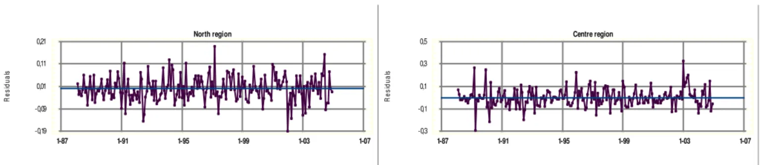
Figure 5. Graph of the residuals for model M1, for the two regions.

From the analysis of Figure 5, some atypical residuals can be noted for the North region for the years

1992, 1997, 2001, 2002 and 2004, as well as some fluctuations in the months of March and April. This

last occurrence may be due to the fact that Easter is a movable holiday. As far as the residuals

corresponding to the year 1992 (July and August) are concerned, these may be justified by the Gulf

War, and, in the case of 1997, for the same months, by the instability of the Russian market and the

conflict in the Balkans. For 2001, the behaviour of the residuals may be based on the fact that, in that

year, the city of Porto was the European Capital of Culture, as well as the fact that the historic centre

of the city of Guimarães and the Alto Douro Wine Region had been classified by UNESCO as World

Cultural Heritage sites. These two factors undoubtedly aroused the curiosity of both Portuguese and

foreign tourists, encouraging them to visit the North region. Once UEFA’s decision to make Portugal

the host country for EURO2004 - the European Football Championship - became known, and after the

aggressive promotional campaign in other European countries had begun in earnest in 2002, a

possible justification can be found for the behaviour of the residuals for 2002 and 2003. In 2004, and

for the months of May and June, coinciding with EURO2004, the behaviour of the residuals is justified

by the holding of this sports event, since 5 of the 10 football stadiums used for the tournament are

situated in the North region.

Further based on Figure 5, and now undertaking the analysis for the Centre region, for 1989, 1990

and 1997, the behaviour of the residuals may be justified by the movable Easter holiday, since this

took place in the months of March and April. For June 1992, justification may be found in the Gulf War,

leading tourists to choose the Centre region for their holidays, and in January 2003, the behaviour

may be based on the fact that in recent years the local authorities of the Centre region have been

investing more heavily in the promotion and organisation of cultural events, as well as in creating

better facilities for winter sports, namely skiing and snowboarding, which attract people to the region,

essentially in the winter months.

Thus, since the suitability of the residuals of model M1 had been explained for the two regions, an

overall analysis was made of the residuals using Box-Pierce statistics. For the model of the North

region and for the lag 24, the Q-value was 16.6893 and the p-value 0.780268; for the model of the

Centre region and for the lag 24, the Q-value was 25.5231 and the p-value was 0.272722. It may

therefore be concluded that one can accept the idea that the residuals of the estimated models follow

the pattern of a white noise since the p-values associated with the Box-Pierce contrast test are

different from zero.

North region

R

e

s

id

u

a

ls

1-87 1-91 1-95 1-99 1-03 1-07 -0,19

-0,09 0,01 0,11

0,21 Centre region

R

e

s

id

u

a

ls

1-87 1-91 1-95 1-99 1-03 1-07 -0,3

To sum up, bearing in mind the different criteria analysed for the assessment of the models, it may be

said that, for each of the regions, the models are expressed by the following equations:

(

)

(

)

[

] [

]

12

1 12

1 12

1 0, 654218

1 0, 757521

12, 2346

16, 9835

t

MRN

LRN

B

B

e

t

t

= ∇∇

=

−

−

=

=

[8]

(

)

₍

₎

[

] [

]

12

1 12

1 12

1 0, 602289

1 0, 662380

10, 9842

12, 7284

t

MRC

LRC

B

B

e

t

t

= ∇∇

=

−

−

=

=

[9]

It should be stressed that this provides conclusive proof that the most appropriate model for capturing

the behaviour of a series is forecasting, which in this way determines the effectiveness of the study.

This procedure will be undertaken in section 2.4.

2.3.2. The Artificial Neural Networks Model

The ANN model selected for the case study of each of the series DRN, North region, and DRC, Centre

region, was of the multi-layer type, in which three layers are used: input layer, hidden layer and output

layer, with a structure of the feedforward type. The logistic sigmoidal activation function [Logsig] was

used in the hidden layer, while the linear activation function was used in the output layer, as this is the

one that provides the best results for architectures of this type. The resilient backpropagation

algorithm, a variant of the backpropagation training algorithm, was used for training the network. The

selection of this algorithm was based on the fact that it had produced satisfactory results in studies

undertaken by the authors Fernandes (2005) and Fernandes and Teixeira (2007). The networks used

in this study have the following architecture: 12 nodes in the input layer, corresponding to the last 12

values of the series, 4 nodes in the hidden layer and 1 in the output layer, corresponding to the

forecast of the value for the following month, or in other words (1-12;4;1). The estimation/forecast was

produced on a monthly basis, i.e. it is a one-step-ahead forecast. The training process used for

updating the weights was the batch training method.

The time series with the original data were divided into three distinct groups: the training group (the

first 216 observations for the DRN series and 216 observations for the DRC series, considering that

the observations used for the validation were not considered in the training); the validation group (12

observations, corresponding to the year 2004 for the DRN series; for the DRC series the observations

used were: January 1999, February 2004, March 2002, April 1996, May 2003, June 2000, July 1998,

August 2004, September 1997, October 2001, November 1994 and December 2003; it was decided to

extract these observations for the DRC series as they were believed to be a ‘good’ representation of

the total group, given its behaviour and because of the authors’ knowledge of the phenomenon under

analysis); and the test group (24 observations, corresponding to the years 2005 and 2006).

It should be stressed that a pre-processing was undertaken of the input data and output data,

corresponding only to a normalisation between -1 and 1, for both series. After this processing, each of

the series was trained with the introduction of more variables into the models, the highest value of the

satisfactory results were obtained, besides the use that was made of the variables mentioned earlier,

the drift - difference - of the peaks was also included in the model. Again, no satisfactory results were

obtained for the validation group, for both series, so that it was decided to use another type of

pre-processing, passing to the logarithmic domain. Improvements were noted in the final results produced

for the two series, although these improvements were not significant in the case of the DRC series.

Since the problem for the DRN series had been solved - minimised - another pre-processing

procedure had to be tried for the DRC series, with the aim of “cleaning” this series. It was therefore

decided to apply a simple differencing and another seasonal differencing to the series in the

logarithmic domain, or, in other words, successive transformations and differencings were applied

between the observations separated by the seasonal period (every 12 months). More satisfactory

results were obtained, transforming the DRC series into a new series. In this way, the new series that

served as a basis for the whole study were: the DRN series in the logarithmic domain and the DRC

series in the logarithmic domain with the application of one simple and another seasonal differencing.

For each of the situations described earlier, 250 training sessions were realised, selecting the results

from the best training session and choosing the ANN with the best results in the validation group, for

each of the series. It should also be mentioned that the validation group was used for each of the

series, to interrupt learning iterations when the performance in this group did not improve after 5

successive iterations. The realisation of several training sessions is justified because the initial values

of the weights are different in each training session, with different solutions also being arrived at, so

that these may have significantly different performances. The criterion used for choosing the best

model, for each of the series under analysis, was the root mean square error (RMSE6) in comparing

the results obtained by the network with the values observed.

The different choices tried out and described in the previous paragraphs were based on the research

work undertaken by Faraway and Chatfield (1998), Thawornwong and Enke (2004), Fernandes

(2005), Fernandes and Teixeira (2007).

2.4. Forecasting Tourism Demand and Performance Evaluation

In this section, the results for the test group (years 2005 and 2006) will be analysed, comparing the

values observed with the values forecast for the two series and using the two methodologies. Later,

the forecasts produced for the years 2005 and 2006 will also be analysed and compared with the

nights spent in hotel accommodation per month recorded during these same years. It should be

mentioned that the forecasting for the months of the years 2005 and 2006 was undertaken without

using as an input any value observed for the year in question. Instead, the values previously forecast

for that year were used as the inputs corresponding to the months of that year. Equations [4] and [5]

were the ones used for calculating the forecasts for each of the methodologies used, Box-Jenkins and

6

(

)

2

1

; : , ; , ; , .

n

t t

t

t t

A P

RMSE where A original value in the period t P forecast value in the period t n total number of observation used n

=

Artificial Neural Networks, respectively, which furthermore were based on the inverse process of the

transformations made.

Through this analysis, the aim was to check whether the models found continue to accompany the

oscillations of the series and to produce acceptable forecasts for tourism demand, for the regions

under study.

Thus, with the aim of observing whether the chosen model produces acceptable forecasting errors,

the following criteria will be calculated for the forecasting errors: absolute percentage error (APE) and

the mean absolute percentage error (MAPE), given by the equations:

; , , .

t t

t t

t

Y P

APE Y observed value and P forecast value

Y

−

= _[10]

1

1

;

,

,

.

n

t t

t t

t t

Y

P

MAPE

Y observed value and P forecast value

n

=

Y

−

=

_[11]

The criterion adopted for analysing the quality of the values forecast with each of the models was

based on the MAPE classification proposed by Lewis (1982), which is presented in the following table.

Table 2. MAPE Criterion for the Assessment of a Model, Lewis (1982).

MAPE (%) Classification of the Forecasts

<10 High Accuracy

10-20 Good Accuracy

20-50 Reasonable Accuracy

>50 Unreliable

With the aim of assessing the model’s predictive capacity, forecasts were made for the years 2005

and 2006, which can be seen in Figure 6 and Table A.3, in the Appendix. If we analyse this figure, it

can be seen that the values estimated by the models accompany the behaviour of the original series,

or, in other words, the models obtained succeed in accompanying the oscillations of the series with

the number of Nights Spent per Month in Hotel Accommodation in both the North region and the

Centre region of Portugal. However, for both regions, there was a significant gap in some months

between the forecast values and those that were actually observed, which makes it possible to say the

Figure 6. Original Nights Spent and Prediction Tourism Demand with ARIMA and ANN models, for both regions, in the period 2005:01 to 2006:12.

Presented in Table 3 are the values of the absolute percentage error (APE) and the mean absolute

percentage error (MAPE). From the analysis of the error values and also based on the criteria

established by Lewis (1982) and presented in Table 2, it may be said that the models successfully

produced highly accurate forecasts for 2005, since the MAPE has values of lower than 10%, for each

of the models. However, for 2006, whilst the Artificial Neural Networks model continued to present

highly satisfactory values of lower than 10%, for both regions, the same did not occur when the values

of the ARIMA model were analysed. Despite presenting satisfactory values, which can be fitted into

the interval that makes it possible to classify the forecasts as displaying “Good Accuracy”, when

compared with those from the Artificial Neural Networks model, these same values were slightly

increased. When the MAPE was calculated for the test group (including the years 2005 and 2006), for

each of the regions, it was seen that, for the North region, the ARIMA model presented a value of

9.39% and the Artificial Neural Network model one of 7.79%. Similar values were also produced for

the Centre region, 9.48% and 7.80%, for the ARIMA model and the Artificial Neural Networks model,

respectively. This fact is interesting, given that, for example, the artificial neural networks models

constructed for each of the regions were subjected to different pre-processing procedures, despite

their having used the same network. It would be interesting to continue to apply this methodology in

future studies, with the aim of observing whether the constructed models continue to display the same

behaviour.

It should further be stressed that some of the values recorded for the APE, for the years 2005 and

2006 and for both regions, were higher than 10% and 20%, resulting from the fact that the models

showed some difficulty in making good forecasts whenever events occurred that caused them to

significantly alter the observed values, despite their continuing to be classified as reliable forecasts.

These facts may, for example, be a consequence of the high level of promotion in international

markets that has been afforded to the regions under analysis. At the same time, local authorities have

also invested more heavily in the promotion and organisation of cultural events and the holding of

theme-based trade fairs, amongst other events. For the North region, investments were made in the

promotion of some tourist destinations, such as the Douro International Natural Park and the Alto

Douro Wine Region, while, in the Centre region, attention was paid to promoting and investing in the

creation of better facilities for winter sports, namely skiing and snowboarding, which attract people to

0 100,000 200,000 300,000 400,000 500,000 600,000 J a n _ 0 5 M a r_ 0 5 M a y _ 0 5 J u l_ 0 5 S e p _ 0 5 N o v _ 0 5 J a n _ 0 6 M a r_ 0 6 M a y _ 0 6 J u l_ 0 6 S e p _ 0 6 N o v _ 0 6 M onths N ig h ts S p e n t p e r M o n th -C e n tr e R e g io n

DRC ARIMA Model ANN Model

0 100,000 200,000 300,000 400,000 500,000 600,000 J a n _ 0 5 M a r_ 0 5 M a y _ 0 5 J u l_ 0 5 S e p _ 0 5 N o v _ 0 5 J a n _ 0 6 M a r_ 0 6 M a y _ 0 6 J u l_ 0 6 S e p _ 0 6 N o v _ 0 6 M onths N ig h ts S p e n t p e r M o n th -N o rt h R e g io n

the region, essentially in the winter months. Since they were not incorporated into the models, all

these factors mean that the models themselves have some difficulty in producing forecasts that lead to

a very low APE, so that mechanisms need to be created that make it possible to minimise errors, such

as, for example, working with intervention variables.

Table 3. Comparison of Prediction Accuracies, in the period 2005:01 to 2006:12.

North Region Centre Region

2005 2006 2005 2006

Months

ARIMA (APE)

ANN (APE)

ARIMA (APE)

ANN (APE)

ARIMA (APE)

RNA (APE)

ARIMA (APE)

ANN (APE)

January 7.4% 8.5% 3.9% 4.8% 11.9% 8.2% 25.8% 12.6%

February 11.2% 9.0% 3.8% 5.8% 15.9% 1.1% 14.9% 1.9%

March 4.5% 10.7% 2.3% 1.1% 8.8% 9.9% 21.3% 2.5%

April 10.0% 6.0% 20.2% 18.9% 7.4% 8.1% 0.2% 1.9%

May 5.8% 5.0% 12.6% 12.4% 6.1% 10.5% 9.6% 2.6%

June 5.8% 8.5% 2.3% 5.8% 6.6% 12.7% 19.0% 19.4%

July 7.8% 5.0% 11.9% 3.2% 1.5% 4.9% 8.0% 1.8%

August 6.9% 11.8% 14.1% 21.0% 2.3% 8.0% 5.6% 8.0%

September 7.5% 1.4% 9.7% 10.6% 6.2% 11.3% 7.3% 14.8%

October 4.1% 4.0% 13.4% 4.6% 8.6% 7.4% 7.3% 4.0%

November 5.4% 1.8% 13.0% 2.0% 8.9% 6.5% 13.5% 9.0%

December 15.8% 11.0% 26.1% 14.2% 5.8% 0.8% 4.8% 19.5%

MAPE 7.7 6.9 11.1% 8.7% 7.5 7.4 11.4% 8.2%

From the analysis carried out previously, it was seen that there is only a slight difference between the

values obtained for the MAPE, with the two models constructed with the different methodologies and

for both regions. It may, however, be inferred that the Artificial Neural Networks models presented

satisfactory statistical and adjustment qualities, showing themselves to be suitable for modelling and

forecasting the reference series, when compared with the models produced by the Box-Jenkins

methodology, or, in other words, the Artificial Neural Networks methodology may be considered an

alternative to the classical Box-Jenkins methodology, in the analysis of tourism demand.

4. Conclusion and Future Work

Portugal has had a similar experience to other countries where tourism has been an activity that

generates wealth and plays an increasingly significant role in the country’s economy.

In such a context, the public or private organisations that are closely linked to the tourism sector and

have been implemented in the regions under study (the North and Centre regions of Portugal) must

devote their energies to building mechanisms that allow them to anticipate the evolution of tourism

demand, with the aim of creating favourable conditions for visitors to these tourist destinations.

This research has sought to investigate and highlight the usefulness of the ANN methodology as an

alternative to the Box-Jenkins methodology, as well as to construct models with these two

methodologies that make it possible to analyse and forecast tourism demand for the regions under

study. The data predicting future national and international tourist flows, i.e. nights spent by tourists in

hotel accommodation for the years 2005 and 2006, were presented and analysed, and then compared

methodology, for the two regions under analysis, the

₍

_{) (}

₎

12

ARIMA 0,1,1 × 0,1,1 model was the one that

was best suited to analysing the behaviour of the reference series, for both regions, making it possible

to produce forecasts for the variable of tourism demand. Although they had distinct pre-processing

procedures, the models constructed with the ANN methodology were based on a feedforward

structure and trained with the resilient backpropagation algorithm, while the logistic sigmoidal

activation function was used, with four neurones in the hidden layer. Each value of the series depends

directly on the twelve preceding values. The forecasts were made monthly. The models obtained with

the ANN methodology present quite satisfactory values, closely following the behaviour of the series

that formed the basis for this study.

Thus, in view of the analysis that was carried out, it was concluded that the models obtained, for the

two methodologies and for both regions, are valid for the sets of data that were used as a support and

presented satisfactory statistical and adjustment qualities, showing themselves to be suitable for

modelling and forecasting the reference series. Results show that the neural network methods with

prior data processing in time series forecasting perform better compared to the Box-Jenkins method,

which made it possible to infer that they can be considered an alternative to the Box-Jenkins

methodology. Since the models showed some difficulty in making good forecasts for some events, it is

suggested that these should be included in the model in the future, for example using intervention

variables for this purpose. This is a challenge that the authors propose to take up in future research,

with the aim of obtaining forecasts that are closer to those that are actually recorded and thus

ensuring greater accuracy for the models.

References

Bishop, C. M.. (1995). “Neural Networks for pattern recognition”. Oxford University Press. Oxford. London.

Chu, Fong-Lin. (1998). “Forecasting Tourist Arrivals: nonlinear sine wave or ARIMA?”. Journal of Travel Research. Vol. 36; pp.79/84.

Faraway, Julian and Chatfield, Chris. (1998). “Time series forecasting with neural networks: a comparative study using the airline data”. Applied Statistics. N.º47, pp.231/250.

Fernandes, Paula O. and Cepeda, Francisco J.T.. (2000). “Aplicação da Metodologia de Box-Jenkins à Série Temporal de Turismo: Dormidas Mensais na Região Norte de Portugal”. Actas do VII Congresso da Associação Portuguesa de Desenvolvimento Regional. Volume I. Universidade dos Açores; Ponta Delgada, Açores, Portugal; pp. 261/272. ISBN:972-97825-8-X.

Fernandes, Paula O. and Teixeira, João Paulo. (2007). “A new approach to modelling and forecasting monthly overnights in the Northern Region of Portugal”. Proceedings of the 4th International Finance Conference. Université de Cergy; Hammamet, Medina, Tunísia.

Hansen, J. V., Mcdonald, J. B. and Nelson, R. D. (1999). “Time series prediction with genetic-algorithm designed neural networks: an empirical comparison with modern statistical models”. ComputlIntell. N.º15, pp. 171/184.

Haykin, Simon. (1999). “Neural Networks. A comprehensive foundation”. New Jersey, Prentice Hall.

Hill, T.; O’connor, M. and Remus, W. (1996). “Neural network models for time series forecasts”. Management Science. Vol. 42 (7), pp. 1082/1092.

INE. Anuários Estatísticos do Turismo de 1987 e 2006. Lisboa, Portugal.

Lewis, C.D. (1982). “Industrial and Business Forecasting Method”. Butterworth Scientific. London.

Murteira, Bento J.F.; Müller, Daniel A. e Turkman, K. Feridun. (1993). “Análise de sucessões cronológicas”. McGraw-Hill; Lisboa.

Otero, José Mª. (1993). “Econometría - series temporales y predicción”. Editorial AC; Madrid.

Parra, S. B. and Domingo, J. U.. (1987). “Análisis de series temporales de turismo de la Comunidad Valenciana”. Estadística Española. N.º114, pp.111/132.

Pulido, Antonio. (1989). “Predicción Económica y Empresarial”. Ediciones Pirámide; Madrid.

Rodrigues, Pedro João S. (2000). “Redes neuronais aplicadas à segmentação e classificação de leucócitos em imagens”. Dissertação de Mestrado em Engenharia Electrónica e Telecomunicações. Universidade de Aveiro.

Rumelhart, D. E. and McClelland, J. L.. (1986). “Parallel Distributed Processing: Explorations in the Microstructure of Cognition”. Volume 1: Foundations. The Massachusetts Institute of Technology Press, Cambridge.

Thawornwong, S. and Enke, D. (2004). “The adaptive selection of financial and economic variables for use with artificial neural networks”. Neurocomputing. N.º6, pp. 205/232.

Witt, Stephen F. and Witt, Christine A.. (1995). “Forecasting tourism demand: a review of empirical research”. International Journal of Forecasting. N.º 11, pp.447/475.

Wong, K. F.. (2002). “Introduction: Tourism Forecasting State of the Art”. Journal of Travel and Tourism Marketing; N.º 13 (1/2), pp.1/3.

Yu, Gongmei and Schwartz, Zvi. (2006). “Forecasting Short Time-Series Tourism Demand with Artificial Intelligence Models“. Journal of Travel Research. N.º 45, pp. 194/203.

A

PPENDIX

A

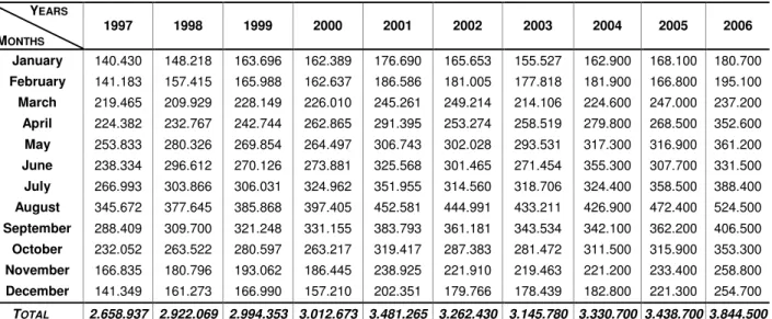
Table A.1. Value of the Original Series, for the period between 1987:01 and 1996:12, North region (cont.).

YEARS

MONTHS

1987 1988 1989 1990 1991 1992 1993 1994 1995 1996

January 102.447 118.011 122.217 126.671 126.826 124.194 121.469 118.606 122.480 126.910

February 102.123 117.547 116.837 129.802 131.653 127.474 129.284 122.988 130.393 139.403

March 125.401 142.687 160.658 158.701 188.999 157.536 154.734 175.261 156.645 172.393

April 150.042 167.118 169.326 197.757 182.290 196.087 189.142 185.525 209.263 213.973

May 180.430 189.823 199.158 207.876 219.187 223.918 198.402 232.075 218.666 239.142

June 197.113 207.729 218.595 227.159 251.295 207.907 207.216 248.237 222.720 245.264

July 229.293 254.523 252.634 257.633 273.927 231.801 231.453 246.274 247.589 248.398

August 304.847 315.113 329.014 351.500 341.490 312.026 304.576 322.366 320.750 336.086

September 238.542 258.287 278.074 284.867 283.378 259.023 249.583 266.094 269.433 280.769

October 173.503 174.359 189.664 216.286 197.241 205.400 202.792 206.256 196.466 225.734

November 130.187 137.933 138.683 162.062 152.554 149.289 141.976 144.803 152.340 175.438

December 114.229 128.774 127.730 139.683 132.802 130.963 120.748 139.706 140.643 143.163

TOTAL 2.048.157 2.211.904 2.302.590 2.459.997 2.481.642 2.325.618 2.251.375 2.408.191 2.387.388 2.546.673

Table A.1. Value of the Original Series, for the period between 1997:01 and 2006:12, North region.

YEARS

MONTHS

1997 1998 1999 2000 2001 2002 2003 2004 2005 2006

January 140.430 148.218 163.696 162.389 176.690 165.653 155.527 162.900 168.100 180.700

February 141.183 157.415 165.988 162.637 186.586 181.005 177.818 181.900 166.800 195.100

March 219.465 209.929 228.149 226.010 245.261 249.214 214.106 224.600 247.000 237.200

April 224.382 232.767 242.744 262.865 291.395 253.274 258.519 279.800 268.500 352.600

May 253.833 280.326 269.854 264.497 306.743 302.028 293.531 317.300 316.900 361.200

June 238.334 296.612 270.126 273.881 325.568 301.465 271.454 355.300 307.700 331.500

July 266.993 303.866 306.031 324.962 351.955 314.560 318.706 324.400 358.500 388.400

August 345.672 377.645 385.868 397.405 452.581 444.991 433.211 426.900 472.400 524.500

September 288.409 309.700 321.248 331.155 383.793 361.181 343.534 342.100 362.200 406.500

October 232.052 263.522 280.597 263.217 319.417 287.383 281.472 311.500 315.900 353.300

November 166.835 180.796 193.062 186.445 238.925 221.910 219.463 221.200 233.400 258.800

December 141.349 161.273 166.990 157.210 202.351 179.766 178.439 182.800 221.300 254.700

Table A.2. Value of the Original Series, for the period between 1987:01 and 1996:12, Centre region (cont.).

YEARS

MONTHS

1987 1988 1989 1990 1991 1992 1993 1994 1995 1996

January 48.413 53.251 60.593 66.389 67.712 72.006 73.457 69.142 70.798 69.186

February 53.932 66.257 70.923 78.898 81.963 78.873 82.466 80.463 81.326 89.418

March 67.949 84.982 118.949 91.836 114.931 98.200 93.210 101.582 104.727 110.697

April 88.730 97.751 88.999 121.039 112.756 124.425 125.441 113.765 139.292 145.682

May 103.595 112.881 122.323 125.580 130.316 141.334 127.772 125.687 133.419 142.172

June 111.331 120.029 126.325 138.110 140.715 121.020 122.687 125.656 130.530 141.044

July 154.594 167.631 182.117 183.161 175.843 163.168 158.791 166.728 164.749 166.283

August 233.117 240.183 263.974 259.879 267.754 247.192 247.527 250.555 242.433 241.940

September 168.602 176.127 190.951 190.030 193.701 175.842 176.980 177.707 171.988 187.513

October 106.730 107.174 118.864 127.891 123.425 121.295 118.980 116.944 116.247 137.972

November 62.249 67.058 75.367 83.646 85.675 84.867 72.739 80.985 80.925 100.324

December 58.618 67.540 94.352 82.305 76.662 78.134 72.227 81.664 97.189 93.096

TOTAL 1.257.860 1.360.864 1.513.737 1.548.764 1.571.453 1.506.356 1.472.277 1.490.878 1.533.623 1.625.327

Table A.2. Value of the Original Series, for the period between 1997:01 and 2006:12, Centre region.

YEARS

MONTHS

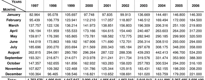
1997 1998 1999 2000 2001 2002 2003 2004 2005 2006

January 82.964 95.078 105.697 97.748 97.835 99.913 136.669 144.481 146.800 146.300

February 95.439 106.779 123.941 112.210 117.057 118.807 146.512 169.494 172.000 184.500

March 137.757 122.126 136.214 141.973 138.851 156.803 196.309 206.316 251.100 219.800

April 136.194 151.959 155.533 173.166 164.615 154.440 240.487 263.603 264.200 317.200

May 159.817 176.390 165.865 173.781 168.582 172.775 282.940 290.185 299.900 320.500

June 144.019 173.863 169.182 167.906 171.690 172.701 256.314 308.510 293.000 294.000

July 185.696 200.270 203.694 211.569 200.343 185.184 297.678 308.175 348.200 358.000

August 262.815 294.081 280.780 296.264 287.122 288.336 439.293 442.413 496.700 534.200

September 193.321 216.871 214.071 213.978 211.241 211.734 319.576 331.474 353.900 388.300

October 147.357 162.655 161.856 162.932 163.283 158.020 257.783 300.534 294.200 316.100

November 107.827 109.382 122.468 131.786 125.344 125.915 183.431 182.155 198.200 208.200

December 100.364 96.465 108.546 116.821 110.652 108.691 161.020 163.759 179.200 221.000

TOTAL 1.753.570 1.905.919 1.947.847 2.000.134 1.956.615 1.953.319 2.918.012 3.111.099 3.297.400 3.508.100

Table A.3. Values Forecast for the Models, for the period between 2005:01 and 2006:12.

North Region Centre Region

Year 2005 Year 2006 Year 2005 Year 2006

ARIMA Model

ANN Model

ARIMA Model

ANN Model

ARIMA Model

ANN Model

ARIMA Model

ANN Model

January 180.579 173.626 182.389 189.349 164.330 158.907 184.061 164.766

February 185.481 187.654 181.870 183.731 199.311 173.894 212.067 187.964

March 235.924 242.683 220.635 234.591 228.927 226.225 266.561 225.229

April 295.228 281.367 284.692 285.916 283.693 285.479 317.873 311.094

May 335.197 315.652 301.171 316.248 318.323 331.353 351.116 328.840

June 325.419 323.895 333.732 312.298 312.205 330.240 349.908 351.012

July 330.532 342.132 340.731 376.036 342.810 331.239 386.499 351.520

August 440.017 450.663 416.740 414.580 508.285 456.970 564.198 491.349

September 389.361 367.067 357.019 363.306 375.764 313.744 416.813 330.920

October 302.841 305.864 328.557 337.129 319.465 315.830 339.159 328.694

November 220.912 225.089 237.594 264.057 215.853 185.341 236.406 189.486

December 186.379 188.159 196.989 218.612 189.648 177.854 210.464 177.856