Exponential Smoothing Method of Base Flow Separation and Its Impact on Continuous Loss Estimates

ISSN 1553-345X

© 2008 Science Publications

Corresponding Author: Dr. G. A Tularam, Griffith University, Griffith School of Environment, Nathan Campus,

Kessels Rd, Brisbane 4111, Australia Tel: 0410649736 Fax: 617 37357459

Exponential Smoothing Method of Base Flow Separation and Its Impact on Continuous

Loss Estimates

1

Gurudeo Anand Tularam and

Mahbub Ilahee

1

Lecturer-Mathematics and Statistics, Faculty of Science Environment Engineering

and Technology, Griffith University (ENV), Brisbane, Australia

2

Fellow- Faculty of Science Environment Engineering

and Technology (ENV),Griffith University, Brisbane Australia

Abstract: The calculation of loss is vital for design flood estimation models and in order to estimate continuing loss (CL), proportional loss (PL) and volumetric runoff coefficient, the surface runoff has to be separated from the total given in a stream flow hydrograph. To obtain the volume of surface runoff from the streamflow hydrograph, baseflow separation becomes necessary and in this paper a few base flow separation methods are explored and an appropriate method selected to assess to impact of baseflow on loss estimates. The process of separation requires a base flow separation coefficient and this coefficient ( ) is selected from individual study catchments from 3 to 5 rainfall streamflow events of the same catchments based on sensitivity analysis. The selected value of individual catchments is then applied to other rainfall streamflow events of a given catchment. It has been observed that a small degree of error in the selection of value does not seem to affect the estimates of the CL, PL or runoff coefficient. Hence, the more practical base flow separation method used in this paper may be applied to other rural catchments for baseflow separation in design loss studies.

Key words: Baseflow separation, rainfall, streamflow, continuing loss, proportional loss, design floods, loss estimates.

INTRODUCTION

Flood estimation is often required in hydrologic design and has important economic significance particularly for low lying lands that are close to rivers 1,2

. Rainfall-based flood estimation techniques are most commonly adopted in practice and they require a number of inputs/parameters to convert design rainfalls to design floods. Of all the inputs/parameters, loss has been noted as an important parameter. Loss is defined to be the amount of precipitation that does not appear as direct surface runoff 3.

In design flood estimation, the simplified lumped conceptual loss models are generally used because of their simplicity and ability to approximate catchment runoff behaviour4. In Australia, the most commonly adopted conceptual loss model is the initial loss-continuing loss (IL-CL) model4. For a specific part of the catchment, the initial loss occurs prior to the commencement of surface runoff, and thus can be considered to be composed of the interception loss, depression storage and infiltration that occur before the

soil surface saturates3. CL is the average rate of loss throughout the remainder of the storm.

To compute the CL value of any study catchment (including input/losses such as proportional loss and volumetric runoff coefficient) from any observed rainfall event, the total volume of the surface runoff from a selected rainfall event needs to be estimated. The observed streamflow data consists of surface runoff, which results from the same rainfall event and the groundwater flow (baseflow). Hence, it is required to separate the total streamflow into surface runoff and baseflow.

This paper briefly reviews various methods of baseflow separation but proposes an exponential smoothing technique that appears to be a more practical method to be used in design loss studies. The paper also shows how an acceptable baseflow separation coefficient ( ) can be selected for any unregulated rural tropical catchment using a set of 3 to 4 streamflow events. The sensitivity of continuing loss, proportional loss and volumetric runoff coefficient to α _{in base}

discusses the results and develops some conclusions for rainfall engineers.

BASEFLOW SEPARATION METHODS

A number of studies have examined separation of baseflow on the basis of physical properties and chemical properties. Depending upon travel time, the ground water flow is classified as quick flow and baseflow at a given time. Dickinson et al.5 and Hall6 have reviewed the baseflow separation technique from the viewpoint of flood analysis. Shirmohammadi et al.7 used rainfall data in conjunction with streamflow data to determine periods of surface runoff. They assumed that a threshold amount of rainfall is needed to initiate surface runoff and assumptions were made about the duration of surface runoff for any rainfall event. Boughton8 and Lyne and Hollick9 used stream flow partitioning as a basis for rainfall runoff modelling and described a method of partitioning stream flow into quick and slow runoff components on the basis of time.

Pilgrim et al.10 and Kobayashi11 studied the use of specific electrical conductance of stream waters as a means of estimating the proportion of different flow components. Kobayashi12 also used stream temperatures for partitioning flows in an area where snowmelt formed a major part of the flow. Hino and Hasebe13 used isotopes of oxygen as a means of separation. The data used in that study are not readily available for routine partitioning of streamflow, which is the limitation for practical application of these methods. Jackman and Hornberger14 have shown that after applying a non-linear loss function to the rainfall data, the response of a wide range of catchments is well represented by a linear model with two components, interpreted as defining a quick flow and slow flow response to the filtered rainfall.

O’ Loughlin et al.15, Hill16, Nathan and McMahon17 separated the flow components not according to physical sources of runoff but on the basis of travel times. Chapman and Maxwell18 showed that the old flow has many of the characteristics of quick flow, and although the old flow can be modelled by algorithms used for baseflow separation, selection of parameter values requires experimental data from tracer experiments. The old flow is identified as being water that was already in the catchment before the start of rainfall, while the new flow has the similar quality characteristics as the incoming rainfall.

Nathan and McMahon17 compared two baseflow separation techniques, one based on a digital filter and the other on simple smoothing and separation rules. They argued that compared to the smoothed minima

technique the digital filter method is better suited to low baseflow conditions and is more strongly correlated with other low flow indicators.

Lyne et al.19 separated streamflow into quick and slow response components using a recursive digital filter. Also O’Loughlin et al.15, Chapman20, Nathan and McMahon17 and Hill16 have used the similar method for baseflow separation. The adopted filter used is of the form:

(1)

k

f

= is the fitted quick response at the kth sampling instant:

k

y

= is the total streamflow; a = the filter parameter (or factor).

This recursive digital filter method separates stream flow into quick and slow flow using a single parameter in the range of 0.75 to 0.90. Other mathematical filtering methods used in Australia for partitioning streamflow are more complex and use several parameters.

Bethlahmy21 used a method to separate the streamflow into quick flow and baseflow. In that method, the rate of baseflow at any time (Bi) is made equal to the sum of the baseflow rate at the previous time (Bi-1) and an incremental value (Ui).

Bi = Bi-1 + Ui (2)

The incremental values for baseflow and interflow separations were calculated using complex functions of the rate of increase of total flow. The reason behind the calculations of the incremental values is not clearly described.

Rather than using complex functions a simpler exponential smoothing model can be used. The exponentially weighted moving average (EWMA) model as given in Equation 3 appears practically easier to apply when compared to most of the models described. As will be shown in this paper, a variant of the model presented below leads to appropriate results. For example for any time period t, the smoothed value St of a time series data set is found by computing

(3)

where y is the observed value and S the smoothed value. In Equation 3, the parameter is called the smoothing constant. This smoothing scheme begins by

k k 1 k k 1

1

f .f (y y )

2

− −

+ α

= α + −

i i 1 i 1

setting S2 to y1, where Si stands for smoothed observation or EWMA, and y stands for the original observation. The subscripts refer to the time periods, 1 to n. For example for the third period,

and so on; in this model there is no S1 and the first observed value is usually equated to S2; hence, the smoothed series starts with the smoothed value of the second observation.

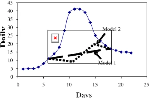
Boughton22 compared two methods of separation of baseflow; namely Model 1 and Model 2 (see Fig. 1). As the method to be chosen for this study ought to be not only acceptable in the literature but must also allow model parameters to be estimated easily from the observed rainfall and/or streamflow data. As Boughton compared two methods of separation of baseflow of which one of them is similar to that described in Eq. 3. Both models allow user identification of a point on a hydrograph at which the separation of flow components is apparent. The methods of partitioning of streamflow can be performed in both ways using daily streamflow data as well as hourly streamflow data for flood hydrograph studies. These methods use manual identification of one or more points that mark the end of surface runoff but differ in assumptions of how base flow discharge increases with the surface runoff.

Model 1 assumes constant rates of baseflow increase with time; that is, the increase in baseflow and the rate of recharge of baseflow depend on time. The overall increase in the rate of baseflow in the streamflow is closely related to the duration of the surface runoff. Model 2 shows that the rate of increase of baseflow depends on the fraction of the surface runoff; that is, the increase in baseflow and the recharge of baseflow depend on runoff volume.

Some studies have shown both models give similar results when simulating large runoff events22 but the main difference between the two models is that Model 1 estimates more surface runoff and less baseflow than

Fig. 1: Comparison of base flow separation by Models 1 and 2

Fig. 2: Baseflow recharge (Models 1 and 2) in large and small runoff events (Y axis is the Daily Discharge (ml)

Model 2 for the large events; while Model 1 estimates less surface runoff and more baseflow than Model 2 for small runoff events. Further, Model 2 estimates some surface runoff at every rise in the hydrograph while Model 1 treats many small rises as increases in baseflow as shown in Figure 2.

Dickson et al.5 illustrated that in the small rises of hydrograph the baseflow discharge shows very quick rise and fall in Model 1, which appears unreasonable. Of these two, Model 2 appears to be a better choice for the general purpose of rainfall-runoff modeling.

More specifically, Model 2 is a form of the single exponential smoothing method as used in time series. It is used to partition the stream flow time series where the rate of increase of the baseflow is made proportional to the rate of surface runoff9,21. In this model, the rate of increase of baseflow depends on the fraction ( ) of the surface runoff (Ai). The rate of baseflow at any time step is Bi, and the separated surface runoff at the same time step is considered to be Ai and the relationship is stated as:

(4)

where; is the stream flow at the same time step of Ai.

Another way of writing the Equation 4 is

(5)

In this research from 50 to 100 years of rainfall and streamflow data were used and a separate computer program was written (in FORTRAN) which fits well with the Boughton21 separation process (Model 2).

4 3 3

S = αy +(1− α)S

0 5 10 15 20 25 30 35 40 45

0 5 10 15 20 25

Days

D

ai

ly

Model 1

Model Model 1

Days

i i l i

B =B− + αA

i i i l i

A =TS −B− ; TS

i i l i i l i i l

After analysing each of the above, a simpler and more practical Boughton’s21 method (Model 2) was used in this study.

This form resembles the single exponential smoothing model normally used in time series. However, the model is different in that base flow observed data is not available in flood modelling excepting the initial value and final (point of inflection) approximated from graphs of daily discharge. This procedure is somewhat similar to that proposed by Robert (1959) who used the observation at time t for this value rather than at time t-1 in Equation 3. Normally, the decision regarding the state of control of the process at any time (t,) depends solely on the most recent measurement from the process. For the EWMA technique as used here, the decision depends on the EWMA statistic, which is an exponentially weighted average of all prior values. By the choice of weighting factor,

α

MATERIAL AND METHODS

The study is based on hourly streamflow and rainfall data. Two medium size rural catchments Bremer River catchment (143110A, catchment area 130 sq km2) and Tenhill Creek catchment (143212A, catchment area 447 sq km2) were selected from Queensland to investigation the baseflow separation from the streamflow. From each catchment four different rainfall streamflow events were selected to estimate an appropriate value for each catchment. Long term rainfall data were purchased from Bureau of Meteorology (BoM) and respective stream flow data were collected from DNRM. The quality of data was checked by BoM and DNRM respectively. A FORTRAN program was developed to investigate the impact on CL due to the separation of baseflow using exponential smoothing method from the stream flow analysis using the equation 4. The output of the FORTRAN program was verified through analytical mathematical calculation and then this computer program was used in this research to compute the total streamflow, baseflow and CL values out of the total rainfall volume.

RESULTS AND DICUSSION

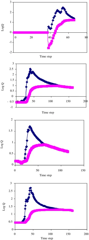
When the streamflow diagram is plotted on a semi-log graph paper, the recession curve (the right section of the graph) of the streamflow diagram becomes a line with constant slope as shown in Fig. 3.

To provide the acceptable baseflow separation from the streamflow the value should be selected in such manner that the baseflow separation line (violet line) can join the start of the recession part of the

Fig. 3: Separation of streamflow components in a semi-log graph for Event 1: when α _{= 0.003,} 0 .004, 0.005, 0.008 (Bremer River)

-4 -3 -2 -1 0 1 2

0 50 100 150

Time step

L

ogQ

-4 -3 -2 -1 0 1 2

0 50 100 150

Time step

L

ogQ

-4 -3 -2 -1 0 1 2

0 50 100 150

Time step

L

ogQ

-4 -3 -2 -1 0 1 2

0 50 100 150

Time step

L

Fig. 4: Baseflow separation with = 0.004 for 3 events in the Bremer River catchment.

streamflow hydrograph; that is, at the start point of the straight line section of the streamflow diagram. Out of many rainfall streamflow events, one rainfall streamflow event was selected and four different values of were used in that event separately to observe the effects of on baseflow separation. The results shown in Figure 3 indicates that a value of = 0.004 provides a more acceptable baseflow separation fit for Event 1, as in this event the straight line part of both the curves are matched together from the point of recession starts (for = 0.005 and = 0.008 both the streamflow and baseflow separation lines merged before point of recession curve starts and for = 0.003 both the

Fig.5: Tenhill Creek catchment: Event 1 when = 0.010 followed by Event 2 when = 0.003; and Event 3 when = 0.008 followed by Event 4 when = 0.002

-0.5 0 0.5 1 1.5 2

0 20 40 60 80

Time step

L

og

Q

-3 -2 -1 0 1 2 3

0 50 100 150

Time step

L

og

Q

-3.5 -3 -2.5

-2 -1.5 -1 -0.5 0 0.5

1

1.5

2

0 _{50 100 150}

Time step

L

og

Q

0 0.5 1 1.5

2

0 50 100 150

Time step

L

og

Q

0 0.5

1 1.5 2 2.5 3

0 50 100 150 200

Time step

L

og

Q

-2 -1 0 1 2 3

0 20 40 60 80

Time step

L

ogQ

-1 - 0.5

0 0.5

1 1.5 2 2.5

3

0 50 100 150 200

Time step

L

o

g

streamflow and baseflow separation lines merged after the point of recession curve starts).

The alpha value selected above for event 1 ( = 0.004) is used to conduct base flow separation for 3 other events in the same catchment. Fig. 4 shows that the value of provides acceptable base flow separation for the other events of the same catchment. This analyses showed that for the Bremer River catchment a value of = 0.004 can be used for baseflow separation for all other streamflow events.

It is worth examining the sensitivity of computed loss values with the change of values. Table 1 shows that for Event 1 in the Bremer River catchment when

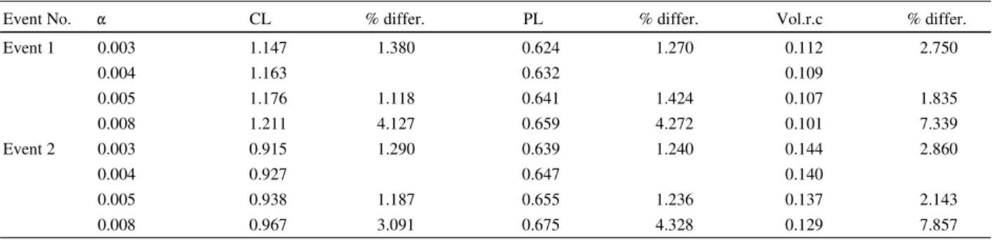
= 0.004, CL = 1.16, if is increased by 25%, the value of CL is varied by 1.11%, if is decreased by 25%, the value of CL is varied by 1.38%. In this manner only 4% variation in CL value was observed due to 100% variation in . This shows that a small error in selection of an appropriate value of does not seem to affect the value of CL significantly for the Bremer River catchment.

Four rainfall stream flow events were selected to estimate an appropriate for Tenhill Creek catchment. In this analysis it was noted that a single value of did not give the acceptable baseflow separation for all the four rainfall streamflow events of the same catchment. It was observed that a value of equals 0.010, 0.003, 0.008 and 0.002 respectively provide acceptable baseflow separation for Events 1, 2, 3 and 4 for Tenhill Creek catchment as shown in Fig. 5.

The selected appropriate value for each event shows a wide variation of baseflow separation with other events and none of these values provided acceptable separation for all the four events. The median of these four values (0.0055) was then explored for separation for all the four events. Figure 6 shows the baseflow separation of the four events with the calculated median = 0.0055; and the figure shows that the use of median value provides a reasonable baseflow separation for all the four events for the Tenhill Creek catchment.

The value of (0.0055) is varied to examining the sensitivity of computed CL values. Table 2 shows that for Event 1 in the Tenhill Creek catchment when

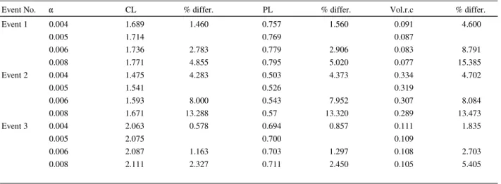
= 0.0055, CL = 1.71, if is increased by 20%, the value of CL is varied by 2.78%, if is decreased by 20%, the value of CL is varied by 1.46%. Thus a 60% variation in the value of resulted in only 4.8% variation in CL value.

Similarly for the Events 2 and 3, the variation in value by about 60% causes about 13% and 2% variation

0 0.5 1 1.5 2

0 50 100 150

Time step

L

o

g

Q

0 0.5

1 1.5

2 2.5

3

0 50 100 150 200

Time step

L

o

g

Q

-2 -1 0 1 2 3

0 20 40 60 80

Time step

L

o

g

Q

0 50 100 150 200 250 300 350

30 40 50 60 70

Time step

Fig. 6: Baseflow separation with = 0.005 for Tenhill Creek [Event 1 and Event 2, Event 3(log scale) followed by Event 3 (natural scale); Event 4 (log scale) followed by Event 4 (natural scale)]

in CL value. However for Event 4, the CL is more sensitive to the change of value (which needs more details analysis). In general it is found that a small error in selecting appropriate value of does not seem to significantly affect the value of CL for the Tenhill Creek catchment.

SUMMARY AND CONCLUSION

In this paper, an adapted exponential smoothing appropriate method of baseflow separation from the streamflow was used to examine the impact of continuing loss for Queensland medium sized rural catchments. The following conclusions can be drawn from this study:

An acceptable baseflow separation coefficient ( ) can be selected for a catchment by trial and error and sensitivity analysis using a small number of stream flow events (3 to 4 streamflow events) without incurring much computational cost;

The continuing loss, proportional loss and volumetric runoff coefficient do not appear to be sensitive to small changes in the chosen value in the baseflow separation. It has been found that a change in by about 50% makes less than 10% variation in the value of continuing loss.

Table 1 Sample events - Effects of changing α value on CL, PL and volumetric runoff co-efficient

Catchment ID = 143110a Catchment name = Bremer River

Event No. CL % differ. PL % differ. Vol.r.c % differ.

Event 1 0.003 1.147 1.380 0.624 1.270 0.112 2.750

0.004 1.163 0.632 0.109

0.005 1.176 1.118 0.641 1.424 0.107 1.835

0.008 1.211 4.127 0.659 4.272 0.101 7.339

Event 2 0.003 0.915 1.290 0.639 1.240 0.144 2.860

0.004 0.927 0.647 0.140

0.005 0.938 1.187 0.655 1.236 0.137 2.143

0.008 0.967 3.091 0.675 4.328 0.129 7.857

-1 -0.5

0 0.5 1 1.5 2 2.5 3

0 50 100 150 200

Time step

L

o

g

Q

0 50 100 150 200 250 300 350 400

0 50 100 150 200

Time step

Table 2: Sample events: Effects of changing value on CL, PL, and volumetric runoff coefficient

Catchment ID = 143212A Catchment name = Tenhill Creek

Event No. CL % differ. PL % differ. Vol.r.c % differ.

Event 1 0.004 1.689 1.460 0.757 1.560 0.091 4.600

0.005 1.714 0.769 0.087

0.006 1.736 2.783 0.779 2.906 0.083 8.791

0.008 1.771 4.855 0.795 5.020 0.077 15.385

Event 2 0.004 1.475 4.283 0.503 4.373 0.334 4.702

0.005 1.541 0.526 0.319

0.006 1.593 8.000 0.543 7.952 0.307 8.084

0.008 1.671 13.288 0.57 13.320 0.289 13.473

Event 3 0.004 2.063 0.578 0.694 0.857 0.111 1.835

0.005 2.075 0.700 0.109

0.006 2.087 1.163 0.703 1.297 0.108 2.703

0.008 2.111 2.327 0.711 2.450 0.105 5.405

ACKNOWLEDGEMENTS

The authors wish to thank the director of the Centre for Environment Systems Research (GU) and Griffith University for funding the research.

REFERENCES

1. Hiscock, K., 2005. Hydrology principles and practice, Blackwell Publishing, Oxford, UK. 2. Snorasson, A., H.P. Finnsdottir, M. Moss, 2002.

The extremes of the extremes: extraordinary floods, IAHS publication no 271, UK, 2002. 3. Institution of Engineers, Australia., 1998.

Australian Rainfall and Runoff. Institution of Engineers, Australia, 1987 and 1998.

4. Hill, P.I., U. Maheepala, R.G. Mein, P.E. Weinmann, Empirical analysis of data to

derive losses for design flood e+-stimation in South-Eastern Australia. CRC for Catchment Hydrology , Report 96/5, 1996.

5. Dickinson, W.T., M.E. Holland and G.L. Smith, 1967. An experimental rainfall-runoff facility. Hydrology paper no. 25, Colorado State University, pp: 78.

6. Hall, A.J., 1971. Baseflow recessions and the baseflow hydrograph separation problem. Hydrology papers 1971, The Institution of Engineers, Australia, pp: 159-170.

7. Shirmohammadi, A., W.G. Knisel and J.M. Sheridan, 1984. An approximate method of

partitioning daily streamflow data. J. Hyd., 74: 335 - 354.

8. Boughton, W.C., 1987. Hydrograph analysis as a basis of water balance modelling. The Institution of Engineers, Australia, Civil Engineering Transaction, CE29(1): 8-33.

9. Lyne, V. D. and Hollick, M., 1979. Stochastic time-variable rainfall-runoff modelling, Institution of Engineers, Australia, Canberra, pp: 89 - 93. 10. Pilgrim, D., D. Huff and T. Steels, 1979. Use of

specific conductance and contact time relations for separating flow components in storm runoff. Water Resources Research, 15(2): 329-339.

11. Kobayashi, D., 1985. Separation of the snowmelt hydrograph by stream temperatures. J. Hyd., 76: 155- 162.

12. Kobayashi, D., 1986. Separation of a snowmelt hydrograph by stream conductance. J. Hyd., 84: 157-164.

13. Hino, M. and M. Hasebe, 1985. Separation of a storm hydrograph into runoff components by both filter separation AR method and environmental isotope tracers. J. Hyd., 85: 251-264.

16. Hill, P.I., 1993. Extreme flood estimation for the Onkaparinga River catchment. M. Eng., Science Thesis, Department of Civil and Environmental Engineering. University of Adelaide, 1993.

17. Nathan, R.J. and T.A. McMahon, 1990. Evaluation of automated techniques for baseflow and recession analysis, Water Resources Research, 26: 1465-1473.

18. Lyne, V.D. and M. Hollick, 1979. Stochastic time-variable rainfall-runoff modelling, Institution of Engineers, Australia, Hydrology and Water Resources Symposium, Perth, pp: 89-92.

19. Chapman, T.G. and A.I. Maxwell, 1996. Baseflow separation-comparison of numerical methods with tracer experiments, Hydrology and Water Resources Symposium, Institution of Engineers, Australia, Hobart, pp: 539-545.

20. Bethalmy, 1974, Smoothing methods in statistics. Springer-Verlag, New York. Or Nist/Ematech., 2007. e-Handbook of Statistical Methods, Engineering statistics hand book. U.S.A.

21. Boughton, W.C., 1988. Partitioning streamflow by computer. The Institution of Engineers, Australia, Civil Engineering Transaction, pp: 285 -291.

22. Roberts, 1959. In Nist/Ematech., 2007. e-Handbook of Statistical Methods, Engineering