Faculdade de Ciˆencias e Tecnologia
Departamento de Engenharia Electrot´ecnica e de Computadores
Design and Performance Evaluation of
Turbo FDE Receivers
Por F´abio J. Silva
Disserta¸c˜ao apresentada na Faculdade de Ciˆencias e Tecnologia da Universidade Nova de Lisboa para obten¸c˜ao do Grau de Mestre em Engenharia Electrot´ecnica e de Computadores.
Orientador: Prof. Doutor Rui Dinis Co-Orientador: Prof. Doutor Paulo Montezuma
To my family and fiancee
It is a pleasure to thank the many people who made this thesis possible.
First and foremost I offer my sincerest gratitude to my supervisors, Prof. Dr. Rui Dinis and Prof. Dr. Paulo Montezuma, who have supported me throughout my thesis with their patience and knowledge, as well as their academic experience, whilst allowing me the room to work in my own way. I attribute the level of my Masters degree to their en-couragement, effort, and belief in my competencies. Without them this thesis would not have been completed or written. I simply could not wish for better or friendlier supervisors.
In my office in the Department of Electrical Engineering and Computers, I was surrounded by knowledgeable and friendly people who helped me daily. I would like to show my grati-tude to my office mates, Andr´e Garrido, Edgar da Silva and Jo˜ao Garcia for being so nice and helpful.
It is an honor for me to thank to my many student colleagues for providing a stimulating and fun environment in which to learn and grow. I am especially grateful to Bruno Alves, David Gon¸calves, Filipe Correia, Pedro Arruda and Tiago Gaspar.
I am very lucky to have the support of many good friends. Life would not have been the same without my friends at the Focolores, Grupo de Jovens das Mercˆes and Temas. Thank you for your never-ending support.
I will always remain grateful to Chiara Lubich for her contribution to peace and unity
among peoples, religions and cultures. “That all may be one.”
I am indebted to my family, especially my parents, Rosa and Paulo, as well as my brother Roberto, who have been a constant source of support – emotional, moral and of course financial – during my graduation years, who taught me to follow my dreams without dis-appointment and fatigue. This thesis would certainly not have existed without them.
Foram desenvolvidas nos ´ultimos anos, diversas t´ecnicas de transmiss˜ao por blocos para sistemas de comunica¸c˜ao sem fios em banda larga, adequadas para lidar com canais forte-mente selectivos na frequˆencia. Nomeadaforte-mente, t´ecnicas como OFDM (Orthogonal Fre-quency Division Multiplexing) e SC-FDE (Single Carrier FreFre-quency Domain Equalization) s˜ao capazes de fornecer ritmos de transmiss˜ao elevados apesar das adversidades do canal. Nesta tese concentramo-nos no estudo da modula¸c˜ao monoportadora, com especial ˆenfase no desenho de estruturas de recep¸c˜ao adequadas a cen´arios caracterizados por canais forte-mente dispersivos no tempo. S˜ao usadas t´ecnicas de transmiss˜ao por blocos assistidas por prefixos c´ıclicos (CP), permitindo implementa¸c˜oes de baixo custo atrav´es do processa-mento de sinal baseado na FFT (Fast Fourier Transform).
´
E investigado o impacto do n´umero de componentes multipercurso, bem como da ordem de diversidade no desempenho assimpt´otico de esquemas SC-FDE.
´
E tamb´em proposta uma estrutura de recep¸c˜ao capaz de realizar um m´etodo de detec¸c˜ao e estima¸c˜ao conjunta, na qual ´e poss´ıvel combinar as estimativas do canal, baseadas em sequˆencias de treino, com as estimativas de canal baseadas no m´etododecision-directed. Finalmente ´e apresentado um estudo sobre o impacto da estima¸c˜ao do factor de correla¸c˜ao no desempenho dos receptores IB-DFE (Iterative Block-Decision Feedback Equalizer).
Palavras Chave: Matched filter bound, OFDM, SC-FDE, Igualiza¸c˜ao no Dom´ınio da Frequˆencia (FDE), Turbo–Igualiza¸c˜ao, Diversidade, Estima¸c˜ao de Canal, Sequˆencias
de Treino, Receptores Iterativos, Estima¸c˜ao do Coeficiente de Correla¸c˜ao.
In recent years, block transmission techniques were proposed and developed for broadband wireless communication systems, which have to deal with strongly frequency-selective fading channels. Techniques like Orthogonal Frequency-Division Multiplexing (OFDM) and Single Carrier with Frequency Domain Equalization (SC-FDE) are able to provide high bit rates despite the channel adversities.
In this thesis we concentrate on the study of single carrier block transmission techniques considering receiver structures suitable to scenarios with strongly time-dispersive chan-nels. CP-assisted (Cycle Prefix) block transmission techniques are employed to cope with frequency selective channels, allowing cost-effective implementations through FFT-based (Fast Fourier Transform) signal processing.
It is investigated the impact of the number of multipath components as well as the diversity order on the asymptotic performance of SC-FDE schemes.
We also propose a receiver structure able to perform a joint detection and channel estima-tion method, in which it is possible to combine the channel estimates, based on training sequences, with decision-directed channel estimates.
A study about the impact of the correlation factor estimation in the performance of Iterative Block-Decision Feedback Equalizer (IB-DFE) receivers is also presented.
Keywords: Matched filter bound, OFDM, SC-FDE, Frequency-Domain Equaliza-tion (FDE), Turbo EqualizaEqualiza-tion, Diversity, Channel EstimaEqualiza-tion, Training Sequences,
Iterative Receivers, Correlation Coefficient Estimation.
Acknowledgements iii
Resumo v
Abstract vii
List Of Acronyms xi
List Of Symbols xviii
List Of Figures xxi
1 Introduction 1
1.1 Motivation an Scope . . . 1
1.2 Objectives . . . 3
1.3 Outline . . . 3
2 Block Transmission Techniques 5 2.1 Multi-Carrier Modulations versus Single Carrier Modulations . . . 5
2.2 OFDM Modulations . . . 8
2.2.1 Transmission Structure . . . 11
2.2.2 Reception Structure . . . 13
2.3 SC-FDE Modulations . . . 17
2.3.1 Transmission Structure . . . 17
2.3.2 Reception Structure . . . 18
2.3.3 IB-DFE Receivers . . . 22
2.4 Comparisons Between OFDM and SC-FDE . . . 25
3 DFE Iterative Receivers 29 3.1 IB-DFE with Hard Decisions . . . 30
3.2 IB-DFE with Soft Decisions . . . 33
3.2.1 Turbo FDE Receiver . . . 35
3.3 Impact of Multipath Propagation and Diversity in IB-DFE . . . 37
3.3.1 Analytical Computation of the MFB . . . 37
3.3.2 Performance Results . . . 40
4 Joint Detection and Channel Estimation 49 4.1 System Characterization . . . 49
4.1.1 Channel Estimation . . . 51
4.2 Decision-Directed Channel Estimation . . . 54
4.3 Performance Results . . . 57
5 Correlation Coefficient Estimation 63 5.1 Method I: Estimation based on the BER estimate . . . 65
5.2 Method II: Estimation based on the LLR . . . 68
5.3 Method III: Estimation based on the MSE . . . 72
5.4 Correlation Coefficient Compensation . . . 76
5.4.1 Method I with Compensation . . . 76
5.4.2 Method II with Compensation . . . 79
5.4.3 Method III with Compensation . . . 81
6 Conclusions and Future Work 85 6.1 Conclusions . . . 85
6.2 Future Work . . . 87
A Minimum Error Variance 89
B Publications 91
ADC Analog-to-Digital Converter AWGN Additive White Gaussian Noise BER Bit Error Rate
CP Cyclic Prefix
CIR Channel Impulsive Response DAC Digital-to-Analog Converter DFT Discrete Fourier Transform DFE Decision Feedback Equalizer FDE Frequency-Domain Equalization FDM Frequency Division Multiplexing FFT Fast Fourier Transform
IB-DFE Iterative Block-Decision Feedback Equalizer IDFT Inverse Discrete Fourier Transform
IFFT Inverse Fast Fourier Transform IBI Inter-Block Interference
ICI Inter-Carrier Interference ISI Inter-Symbol Interference MC Multi-Carrier
MFB Matched Filter Bound
MMSE Minimum Mean Square Error MRC Maximal-Ratio Combining
MSE Mean Square Error
OFDM Orthogonal Frequency-Division Multiplexing PMEPR Peak-to-Mean Envelope Power Ratio PDP Power Delay Profile
PSD Power Spectrum Density PSK Phase Shift Keying
QAM Quadrature Amplitude Modulation QPSK quadrature Phase-Shift Keying SC Single Carrier
SC-FDE Single Carrier with Frequency Domain Equalization SINR Signal to Interference-plus-Noise Ratio
General Symbols
Bk feedback equalizer coefficient for thekth frequency
Eb average bit energy
Es average symbol energy
F subcarrier separation
Fk feedforward equalizer coefficient for thekth frequency
Fk(l) feedforward equalizer coefficient for thekth frequency and lth diversity branch
f frequency variable
fk kth frequency
g(t) impulse response of the transmit filter
Hk overall channel frequency response for the kth frequency ˜
HkL overall channel frequency response estimation for the kth frequency
Hk(l) overall channel frequency response for the kth frequency and lth diversity branch
Hk(m) overall channel frequency response for the kth frequency of themth time block ˜
HkD data overall channel basic frequency response estimation for the kth frequency ˆ
HkD data overall channel enhanced frequency response estimation for the kth frequency ˜
HkT S training sequence overall channel basic frequency response estimation for the kth
frequency ˆ
HT S
k training sequence overall channel enhanced frequency response estimation for the
kth frequency ˜
HkT S,D overall channel basic frequency response combined estimation for thekthfrequency
ˆ
HkT S,D overall channel enhanced frequency response combined estimation for thekth fre-quency
h(τ, t) channel impulse response
hT(t) pulse shaping filter ˜
hD
n data overall channel basic impulsive response estimation for the nth time-domain sample
ˆ
hDn data overall channel enhanced impulsive response estimation for the nth time-domain sample
˜
hT Sn training sequence overall channel basic impulsive response estimation for the nth
time-domain sample ˆ
hT S
n training sequence overall channel enhanced impulsive response estimation for the
nth time-domain sample ˜
hT S,Dn overall channel basic impulsive response combined estimation for the nth time-domain sample
ˆ
hT S,Dn overall channel enhanced impulsive response combined estimation for thenth time-domain sample
i tap index of the diversity branch
k frequency index
L power of 2
LIn(i) in-phase log-likelihood ratio for the nth symbol at theith iteration
LQn(i) quadrature log-likelihood ratio for thenth symbol at theith iteration
l antenna index/diversity branch
m data symbol index
N number of symbols/subcarriers
N0 noise power spectral density (unilateral) ND number of data blocks
NRx space diversity order
NT S number of symbols of the training sequence
NkT S training sequence channel noise for the kth frequency
Nk(l) channel noise for the kth frequency and lth diversity branch
Nk(m) channel noise for the kth frequency of the mth time block
NG number of guard samples
n time index
n(t) noise signal
Pb AWGN channel performance
Pb,MFB matched filter bound performance Pe bit error rate
ˆ
Pe estimated bit error rate
R(f) Fourier transform of r(t)
R(τ) autocorrelation function
r(t) rectangular pulse/shaping pulse
S(f) frequency-domain signal
Sk kth frequency-domain data symbol
ST Sk training sequence kth frequency-domain data symbol
S(km) kth frequency-domain data symbol of the mth data block ˜
Sk estimate for the kth frequency-domain data symbol ˜
S(km) estimate for the kth frequency-domain data symbol of the mth data block ˆ
Sk “hard decision” for the kth frequency-domain data symbol ˆ
S(km) “hard decision” for the kth frequency-domain data symbol of themth data block
Sk “soft decision” for the kth frequency-domain data symbol
s symbol of an QPSK constellation
s(t) time-domain signal
s(t)(m) signal associated to themth data block
sI(t) continuous in-phase component
sn nth time-domain data symbol
sIn discrete in-phase component
sQn discrete quadrature component
sT S
n training sequencenth symbol ˜
sn sample estimate of thenth time-domain data symbol ˜
s(nm) estimate of thenth time-domain data symbol of the mth data block ˆ
sn “hard decision” of thenth time-domain data symbol ˆ
s(nm) “hard decision” of thenth time-domain data symbol of themth data block
sn “soft decision” of thenth time-domain data symbol
T duration of the useful part of the block
TB block duration
TCP duration of the cyclic prefix
TD duration of the data blocks
TF frame duration
TG guard period
TT S duration of the training block
Ta sampling interval
Ts symbol duration
t time variable
Ul discrete taps order for thelth diversity branch
Utotal total of discrete taps order forNRx space diversity order
Yk received sample for thekth frequency
YkT S training sequencekth frequency-domain received sample
Yk(m) kth frequency-domain received sample of themth data block
Yk(l) received sample for thekth frequency and lth diversity branch
yn nth time-domain received sample
y(nl) nth time-domain received sample for thelth diversity branch
y(t) received signal
wn nth channel noise sample
α inverse of the SNR
β relation between the average power of the training sequences and the data power ∆(ki) error term for the kth frequency-domain “hard decision” estimate
∆(km) zero-mean error term for thekth frequency-domain “hard decision” estimate of the
mth data block
γ(i) average overall channel frequency response at theith iteration
κ(i) normalization constant for the FDE
ρ(i) correlation coefficient at the ith iteration ˆ
ρ estimated value of ρ
ρEst+Comp compensated correlation coefficient
χ(ˆρ) compensation factor of the correlation coefficient
ρm correlation coefficient of themth data block
ρIn correlation coefficient of the “in-phase bit of thenth data symbol
ρQn correlation coefficient of the “quadrature bit of the nth data symbol
σ2
Eq total variance of the overall noise plus residual ISI ˆ
σ2Eq approximated value of σEq2
σ2MSE mean-squared error (MSE) variance
σ2
N variance of channel noise
σ2
S variance of the transmitted frequency-domain data symbols
σ2H,T S variance of the noise in the channel estimates related with the training sequence
σ2D variance of the noise in the channel estimates related with the data blocks
σ2
ε(ki) global error consisting of the residual ISI plus the channel noise at theith iteration
εEqk (i) denotes the overall error for thekth frequency-domain symbol
ϑI
n error in ˆsIn
ϑQn error in ˆsQn
Ω2i,l mean square value of the magnitude of each tap i for thelth diversity branch
ϕi,l(t) zero-mean complex Gaussian random process
τi,l delay associated to the ith tap and lth diversity branch
δ(t) Dirac function
νl represents AWGN samples
ǫH
kL channel estimation error
ǫD
k data channel estimation error
ǫT S
k training sequence channel estimation error
ǫT S,Dk combined training and data channel estimation error Matrix Symbols
z Utotal×1 vector
zH conjugate transpose of z
Σ Σis aUtotal×Utotal Hermitian matrix z Utotal×1 vector
Rl autocorrelation function matrix ofR(τ) associated to the lth diversity branch Ψ covariance matrix of z
2.1 Conventional FDM . . . 7
2.2 The power density spectrum of the complex envelope of the OFDM signal, with the orthogonal overlapping sub-carriers spectrum (N = 16). . . 10
2.3 MC burst’s final part repetition in the guard interval. . . 11
2.4 Basic OFDM transmitter block diagram. . . 13
2.5 Basic OFDM receiver block diagram. . . 14
2.6 (a) Overlapping bursts due to multipath propagation; (b) IBI cancelation by implementing the cyclic prefix. . . 15
2.7 (a) OFDM Basic FDE structure block diagram with no space diversity; (b) and with an NRx-order space diversity. . . 16
2.8 Basic SC-FDE transmitter block diagram. . . 18
2.9 Basic SC-FDE receiver block diagram. . . 19
2.10 (a) Basic SC-FDE structure block diagram with no space diversity; (b) and with anNRx-order space diversity. . . 21
2.11 (a) Basic IB-DFE structure block diagram with no space diversity; (b) and with anNRx-order space diversity. . . 22
2.12 Uncoded BER perfomance for an IB-DFE receiver with four iterations. . . . 24
2.13 Basic transmission chain for OFDM and SC-FDE. . . 25
2.14 Performance result for uncoded OFDM and SC-FDE. . . 26
3.1 IB-DFE receiver structure employing “soft decisions” from the FDE output in the feedback loop. . . 35
3.2 Improvements in uncoded BER perfomance accomplished by employing “soft decisions” in an IB-DFE receiver with four iterations. . . 36
3.3 SISO channel decoder soft decisions . . . 37
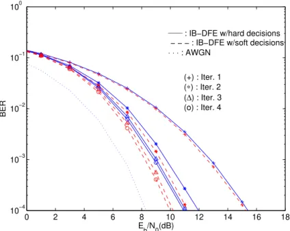
3.4 BER performance for an IB-DFE without channel coding forNRx= 1. . . . 42
3.5 BER performance for an IB-DFE without channel coding forNRx= 2. . . . 42
3.6 BER performance for an IB-DFE without channel coding forNRx= 4. . . . 43
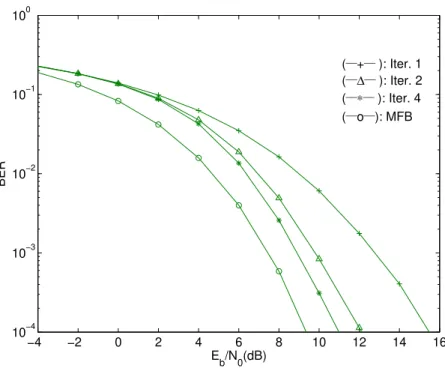
3.7 BER performance for a conventional IB-DFE with channel coding, as well as a turbo IB-DFE forNRx= 1. . . 43
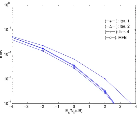
3.8 BER performance for a conventional IB-DFE with channel coding, as well as a turbo IB-DFE for NRx= 2. . . 44 3.9 BER performance for a conventional IB-DFE with channel coding, as well
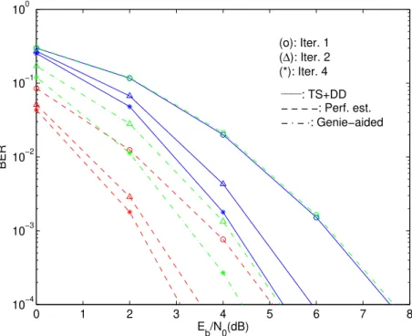
as a turbo IB-DFE for NRx= 4. . . 44 3.10 Required Eb/N0 to achieve BER = 10−4 without convolutional code and
uniform PDP, as function of the number of multipath components: IB-DFE with 1, 2 and 4 iterations; MFB (dashed lines). . . 45 3.11 Required Eb/N0 to achieve BER= 10−5 with convolutional code for
uni-form PDP, as function of the number of multipath components: IB-DFE with 1, 2 and 4 iterations; MFB (dashed lines). . . 46 3.12 Required Eb/N0 to achieve BER = 10−4 without convolutional code for
exponential PDP, as function of the number of multipath components: IB-DFE with 1, 2 and 4 iterations; MFB (dashed lines). . . 46 3.13 RequiredEb/N0 to achieveBER= 10−5 with convolutional code for
expo-nential PDP, as a function of the number of multipath components: IB-DFE with 1, 2 and 4 iterations; MFB (dashed line). . . 47 3.14 Required Eb/N0 to achieve BER = 10−4 without convolutional code for
uniform PDP, without diversity, as a function of the number of multipath components: IB-DFE with 1, 2 and 4 iterations; MFB (dashed line). . . 47 4.1 Frame structure. . . 50 4.2 Impulsive response of the channel estimation. . . 52 4.3 Frequency response of the channel estimation. . . 53 4.4 Combination scheme between ˜HT S
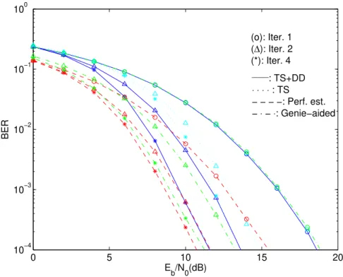
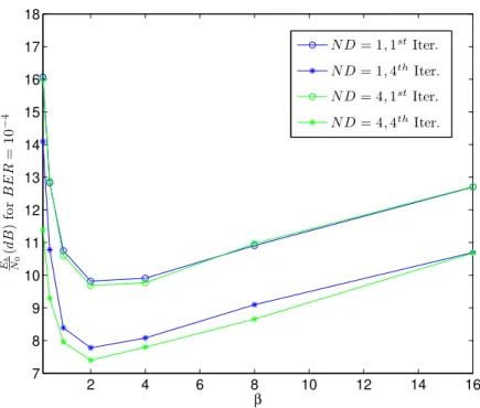
k and ˜HkD channel estimates. . . 55 4.5 Variance of the channel estimates for the k subcarriers, withEb/N0= 20 . . 57 4.6 BER performance for uncoded SC-FDE with ND = 1 block and β= 1. . . . 58 4.7 BER performance for uncoded SC-FDE with ND = 4 blocks andβ = 1. . . 59 4.8 BER performance for coded SC-FDE withND = 1 block and β= 2. . . 59 4.9 BER performance for coded SC-FDE withND = 4 blocks andβ = 2. . . 60 4.10 Required Eb/N0 to achieve BER = 10−4 without convolutional code, as
function of β: IB-DFE with 1 and 4 iterations. . . 60 4.11 RequiredEb/N0 to achieve BER= 10−4 with convolutional code, as
func-tion ofβ: IB-DFE with 1 and 4 iterations. . . 61 5.1 Evolution of ρ as function of theEb/N0 for method I. . . 66 5.2 Evolution of σEq as function of the BER for method I. . . 66 5.3 Evolution of σEq as function of theEb/N0 for method I. . . 67 5.4 BER perfomance for method I. . . 67 5.5 Required BER to achieve Eb/N0 = 9 (dB) as a function of the iterations
5.7 Evolution ofσEq as function of the BER for method II. . . 70 5.8 Evolution ofσEq as function of theEb/N0 for method II. . . 71 5.9 BER perfomance for method II. . . 71 5.10 Required BER to achieve Eb/N0 = 9 (dB) as a function of the iterations
number for method II. . . 72 5.11 Evolution ofρ as function of theEb/N0 for method III. . . 74 5.12 Evolution ofσEq as function of the BER for method III. . . 74 5.13 Evolution ofσEq as function of theEb/N0 for method III. . . 75 5.14 BER perfomance for method III. . . 75 5.15 Required BER to achieve Eb/N0 = 9 (dB) as a function of the iterations
number for method III. . . 76 5.16 Relation between the correlation coefficient estimation and the
compensa-tion factor for method I . . . 77 5.17 Evolution ofρ as function of theEb/N0 for method I. . . 78 5.18 BER perfomance for method I. . . 78 5.19 Required BER to achieve Eb/N0 = 9 (dB) as a function of the iterations
number for method I. . . 79 5.20 Relation between the correlation coefficient estimation and the
compensa-tion factor for method II. . . 79 5.21 Evolution ofρ as function of theEb/N0 for method II. . . 80 5.22 BER perfomance for method II. . . 81 5.23 Required BER to achieve Eb/N0 = 9 (dB) as a function of the iterations
number for method II. . . 81 5.24 Relation between the correlation coefficient estimation and the
compensa-tion factor for method III. . . 82 5.25 Evolution ofρ as function of theEb/N0 for method III. . . 82 5.26 BER perfomance for method III. . . 83 5.27 Required BER to achieve Eb/N0 = 9 (dB) as a function of the iterations
Introduction
1.1
Motivation an Scope
The growing demand for high speed wireless services and applications (especially those based on multimedia) has incited the rapid development of broadband wireless systems. A major challenge in design of this type of mobile communications systems is to over-come the effects of the mobile radio channel, assuring at the same time high power and spectral efficiencies. Therefore, to meet the high data rate requirements while dealing with severely time-dispersive channels effects, equalization techniques at the receiver side become necessary to compensate the signal distortion and guarantee good performance. It is known that the Viterbi [1] equalizer is the optimum receiver to deal with time-dispersive channels. However, its complexity grows exponentially with the length of the Channel Impulsive Response (CIR).
An alternative technique used to minimize the channel frequency selectivity effects is time-domain equalization. In comparison with Viterbi equalizers, time-domain equaliza-tion techniques offer much lower implementaequaliza-tion complexity. However, according to [2], conventional Single Carrier (SC) modulations suffer from a growing complexity with the length of channel response. Moreover, time-domain equalization normally needs a number of multiplications, per symbol, proportional to the maximum channel impulse response length [2].
It is known that nonlinear equalization, such as Decision Feedback Equalizer (DFE) [3], offers better performance for frequency-selective radio channels than linear equalization,
with just a small complexity increase. A nonlinear equalizer is implemented with a linear filter to remove a portion of Inter-Symbol Interference (ISI), followed by a filter that can-cels the remaining interference, using previous detected data. Notwithstanding, when the time length of the channel response increases, conventional time-domain DFE receivers become too complex and more susceptible to error propagation problems.
Multi-Carrier (MC) modulation systems employing Frequency-Domain Equalization (FDE) are an alternative to SC modulation systems. One approach, OFDM, has become popular and widely used in a large number of wireless communications systems which operate in severely frequency-selective fading radio channels. For channels with severe delay spread, OFDM employs frequency domain equalization which is computationally less complex than the corresponding time domain equalization. This is because equalization is performed on a block of data at a time, and the operations on this block involve Discrete Fourier Transform (DFT) implemented by an efficient Fast Fourier Transform (FFT) [4] operation and a simple channel inversion operation.
More recently, SC modulations have recover the interest and became an alternative to MC, due to the use of nonlinear equalizer receivers implemented in the frequency-domain, employing FFTs, which allow better performances than the corresponding OFDM, while keep low the complexity of implementation. Furthermore, SC modulations have shown to be effective for block transmission schemes with cyclic prefix. Moreover, block transmission techniques employing FDE techniques, where each block includes a appropriate Cyclic Prefix (CP) (i.e., with a size that deals with the maximum channel delay), proved to be suitable for high data rate transmission over highly dispersive channels [5] [2], since they require simple FFT operations and the signal processing complexity grows logarithmically with the channel’s impulsive response length.
1.2
Objectives
This thesis focus on the study of SC block transmission techniques with cycle prefix over severely frequency-selective fading radio channels.
It is investigated the impact of the number of multipath components as well as the diversity order on the asymptotic performance of SC-FDE schemes. The simulation’s results show that, for a high number of multipath components, the system’s asymptotic performance approaches the Matched Filter Bound (MFB), even without diversity. When diversity is considered, the performance approaches the MFB faster, even for a small number of multipath components.
We also made a characterization of the channel estimation problem, that includes the pro-pose of a joint detection and channel estimation method, in which it is possible to combine the channel estimates, based on training sequences, with decision-directed channel esti-mates. These systems were evaluated through Monte-carlo simulations, and the obtained system performance results show the good performances allowed by these techniques, even without resort to high-power pilots or training blocks.
A research about the impact of the correlation factor estimation in the performance of IB-DFE receivers is also present. Since the correlation factor represents a key parameter to ensure the good performance of IB-DFE receivers, reliable estimates are needed in the feedback loop. We present several methods to estimate the correlation coefficient. We also propose a technique to compensate the inaccuracy of the correlation coefficient estimation.
1.3
Outline
After this introductory chapter, chapter 2 characterizes the basic principles of SC mo-dulations and their relations with MC momo-dulations. OFDM momo-dulations and SC-FDE modulations with linear and nonlinear equalizer receivers are described, including trans-mitter and receiver schemes as well as the signal’s representation in time and frequency domain.
char-acterized by employing in the equalizer’s feedback loop the “soft decisions” at the channel decoded outputs. It is also investigated the impact of the number of multipath components and diversity order, on the asymptotic performance of IB-DFE schemes. For comparison purposes, are also derived the analytical expressions for the MFB, in a multipath envi-ronment, with or without diversity. Finally, some performance results are presented and discussed.
Block Transmission Techniques
A brief introduction to MC modulations and SC modulations is made in this chapter. This includes several aspects such as the analytical characterization of each modulation type, and some relevant properties of each modulation. For both modulations a special attention is given to the characterization of the transmission and receiver chains, with special emphasis on the transmitter and receiver performance structures. The chapter is organized as follows: In section 2.1, MC modulations and their relations with SC modula-tions are analyzed. Section 2.2 describes the OFDM modulation. Section 2.3 characterizes the basic aspects related with SC-FDE modulation including the linear and iterative FDE receivers. Finally, in section 2.4 we compare the performance of OFDM and SC-FDE for severely time-dispersive channels.
2.1
Multi-Carrier Modulations versus Single Carrier
Modu-lations
Let us start by analyzing a conventional single carrier modulation. With SC schemes we transmit using a single carrier at a high symbol rate. It is a modulation where the energy of each symbol is distributed by the total transmission band. For a linear modulation, the complex envelope of anN-symbol burst (presuming that N is even) can be written as
s(t) = N−1
X
n=0
snr(t−nTs), (2.1)
wheresnis a complex coefficient that corresponds to thenthsymbol, selected from a chosen constellation (for example, a Phase Shift Keying (PSK) constellation, or a Quadrature Amplitude Modulation (QAM)), according to a data sequence and a appropriated mapping rule, r(t) denotes the support pulse and Ts refers the symbol duration. Applying the Fourier transform (FT) to (2.1) we may write
S(f) =F{s(t)}= N−1
X
k=0
snR(f)e−j2πf nTs. (2.2)
Therefore from (2.2), results a transmission band for each data symbol sn equal to the band occupied byR(f), where R(f) denotes the FT of r(t).
By contrast, in a multi-carrier modulation the N symbols are sent in the frequency-domain, each one on a different sub-carrier during the same time intervalT. Therefore, a multi-carrier burst has the following spectrum
S(f) = N−1
X
k=0
SkR(f−kF), (2.3)
whereN refers to the number of sub-carriers,Skrefers to thekthfrequency-domain symbol and F = T1
s denotes the spacing between sub-carriers. Applying the inverse Fourier
transform to both sides of (2.3), leads to the dual of (2.2)
s(t) =F−1{S(f)}= N−1
X
k=0
Skr(t)ej2πkF t, (2.4)
that represents the complex envelope of the corresponding multi-carrier burst. Comparing the equations (2.1) with (2.3) and (2.2) with (2.4), becomes clear that the SC modulations are a dual version of the MC modulations and vice-versa.
The simplest multi-carrier modulation is the conventional Frequency Division Multiplexing (FDM) scheme, where the spectrum related to the different sub-carriers do not overlap. When the bandwidth ofR(f) is smaller thenF1, the bandwidth associated to each symbol
Sk will be a fraction N1 of the total transmission band, as shown in Fig. 2.1.
For a transmission without ISI (InterSymbol Interference), the pulsesr(t) must verify the
1
-4
-5 -3 -2 -1 0 1 2 3 4 5
-4
S S-3 S-2 S-1 S0 S1 S2 S3 S4
... ...
1
f F
()
Sf
Figure 2.1: Conventional FDM
following orthogonality condition
Z +∞
−∞
r(t−nTs)r∗(t−n′Ts)dt= 0, n6=n′. (2.5)
Due to the duality property mentioned above, in the frequency domain, results the or-thogonality condition between sub-carriers given by
Z +∞
−∞
R(f −kF)R∗(f −k′F)df = 0, k6=k′. (2.6)
Using the Parseval’s Theorem, we may write (2.6) as
Z +∞
−∞
|r(t)|2e−j2π(k−k′)F tdt= 0, k6=k′. (2.7)
For the particular case of linear SC modulations, the different pulses given by r(t−nTs) withn=...,−1,0,1, ..., are still orthogonal even when exists overlap between them. For example, the pulse
r(t) =sinc
t Ts
, (2.8)
with sinc(x) , senπx(πx), verifies the condition (2.5). Similarly, for MC modulations the orthogonality is still preserved between the different sub-carriers even when the different
and (2.7)) is verified when
R(f) =sinc
f F
, (2.9)
that corresponds to have in time-domain a rectangular pulse r(t), with duration T = F1. In this case, the orthogonality condition (2.7) becomes
Z t0+T
0
e−j2π(k−k′)F tdt= 0, k6=k′. (2.10)
2.2
OFDM Modulations
OFDM (Orthogonal Frequency Division Multiplexing) [6] is a multi-carrier modulation technique where data is transmitted simultaneously onN narrowband parallel sub-carriers. Each sub-carrier uses only a small portion of the total available bandwidth given byN.F, with a sub-carrier spacing of F ≥ T1
B, where TB denotes the period of an OFDM block.
By contrast to the SC modulation, the OFDM transmits N symbols as a block during each time intervalTB. Consequently, the period of an OFDM block,TB, isN times bigger than the symbol period Ts. It can be viewed as a technique in many aspects similar to FDM, but in OFDM the sub-carriers are separated in frequency by the minimum distance required to fulfill the orthogonality condition between them.
The complex envelope of an OFDM signal is characterized by a sum of bursts (or blocks), with durationTB≥T (whereT = F1 denotes the duration of the useful part of the block), and are transmitted at a rate F ≥ T1
B, i.e.,
s(t) =X m
"N−1 X
k=0
Sk(m)ej2πkF t #
r(t−mTB). (2.11)
It is important to point out that theN data symbols{Sk;k= 0, ..., N−1}are sent during themth block, and that the group of complex sinusoids{ej2πkF t;k= 0, ..., N−1}denotes the sub-carriers.
Let us consider the mth OFDM block. During the OFDM block interval, the transmitted signal can be expressed as
s(m)(t) = N−1
X
k=0
Sk(m)r(t)ej2πkF t = N−1
X
k=0
with the pulse shape,r(t), defined as
r(t) =
1, [−TG, T] 0, elsewhere
, (2.13)
whereT = F1 andTG≥0 denotes the duration of the “guard interval” used to compensate time-dispersive channels. Therefore r(t) consists in a rectangular pulse, which duration should be greater then T (TB = T +TG ≥ T = F1) to be able to deal with the time-dispersive characteristics of the channels. The sub-carrier spacingF = T1, guarantees the orthogonality between the sub-carriers over the OFDM block interval. In spite of the fact that (2.7) is not verified by the pulse given by (2.13), the different sub-carriers are still orthogonal during the interval [0, T], which coincides with the effective detection interval, since
Z T 0
|r(t)|2e−j2π(k−k′)F tdt=
Z T 0
e−j2π(k−k′)F tdt=
1, k=k′,
0, k6=k′. (2.14)
Therefore, for each sampling instant, we may write (2.12) as
s(m)(t) = N−1
X
k=0
Skej2πkF t, 0≤t≤TB. (2.15)
In spite of the overlap of the different sub-carriers, the mutual influence among them can be avoided. This implies a waveform that uses the available bandwidth with a very high bandwidth efficiency. Under these conditions, the bandwidth of each sub-carrier becomes small when compared with the coherence bandwidth of the channel (i.e., the individual sub-carriers experience flat fading, which allows simple equalization). This means that the symbol period of the sub-carriers must be longer than the delay spread of the time-dispersive radio channel.
From (2.4), we can say that themth “burst” (or block) should take the form
s(m)(t) = N−1
X
k=0
Sk(m)ej2πkF t= N−1
X
k=0
S(km)ej2π k TBt=
N−1 X
k=0
Sk(m)ej2πfkt, 0≤t≤T
where{Sk(m);k= 0, ..., N−1}represents the data symbols of themth burst,{ej2πfkt;k=
0, ..., N−1}are the sub-carriers,fk = TkB is the center frequency of thekthsub-carrier, and
r(t) is a rectangular pulse with duration superior to F1, attending to the time dispersion conditions introduced by the channel. It is also assumed that r(t) = 1 in the interval [−TG, T].
By applying the inverse Fourier transform to both sides of (2.16), we obtain
S(f) =F{s(t)}= N−1
X
k=0
S(km)sinc
f− k
TB
, (2.17)
where the center frequency of thekth sub-carrier isfk = TkB, with a sub-carrier spacing of
1
TB, that assures the orthogonality during the block interval (as stated by (2.14)).
Fig. 2.2 depicts the Power Spectrum Density (PSD) of an OFDM signal, as well as the individual sub-carrier spectral shapes for N = 16 sub-carriers and data symbols. As we can see from Fig. 2.2, when the kth sub-carrier PSD (fk = TkB) has a maximum the adjacent sub-carriers have zero-crossings, which achieve null interference between carriers and improves the overall spectral efficiency.
−0.80 −0.6 −0.4 −0.2 0 0.2 0.4 0.6 0.8
0.2 0.4 0.6 0.8 1
fT/N
PSD
____
: Subcarrier − − − −: Overall
Figure 2.2: The power density spectrum of the complex envelope of the OFDM signal, with the orthogonal overlapping sub-carriers spectrum (N = 16).
cyclic prefix instead of a zero interval, it can be shown that we also eliminate Inter-Carrier Interference (ICI) provided that we only use the useful part of the block for detection purposes [7]. Therefore, the equation (2.16) is a periodic function int, with periodT, and the complex envelope associated to the guard period can be regarded as a repetition of the MC bursts final part, as exemplified in Fig. 2.3. Thus, it is valid to write
s(t) =s(t+T), −TG≤t≤0. (2.18)
Consequently, the guard interval is a copy of the final part of the OFDM symbol which is added to the beginning of the transmitted symbol, making the transmitted signal periodic. The cyclic prefix, transmitted during the guard interval, consists of the end of the OFDM symbol copied into the guard interval, and the main reason to do that is on the receiver that integrates over an integer number of sinusoid cycles each multipath when it performs OFDM demodulation with the FFT [4].
CP
G
T
B
T
( )
s t
OFDM block
t T
Figure 2.3: MC burst’s final part repetition in the guard interval.
We may note that the guard interval also reduces the sensitivity to time synchronization problems.
2.2.1 Transmission Structure
sn≡s(t)|t=nTa =s(t)δ(t−nTa) =
N−1 X
k=0 Skej2π
k
TnTa, n= 0,1, ..., N −1, (2.19)
whereF = T1. Consequently, (2.19) can be written as
sn= N−1
X
k=0 Skej
2πkn
N =IDF T{Sk}, n= 0,1, ..., N−1. (2.20)
Hence,{sn;n= 0, ..., N−1}=IDF T{Sk;k= 0, ..., N−1}. At the output of the Inverse Fast Fourier Transform (IFFT), a CP ofNG samples, is inserted at the beginning of each block ofN IFFT coefficients. It consists in a time-domain cycle extension of the OFDM block, with size larger than the channel impulse response (i.e, the NG samples assure that the CP length is equal or greater than the channel length NH). The cycle prefix is appended between each block, in order to transform the multipath linear convolution in a circular one. Thus, the transmitted block is {sn;n = −NG, ..., N −1}, and the time duration of an OFDM symbol is NG+N times larger than the symbol of a SC modu-lation. Clearly, the CP is an overhead that costs power and bandwidth since it consists of additional redundant information data. Therefore, the resulting sampled sequence is described by
sn= N−1
X
k=0 Skej
2πkn
N , n=−NG,1, ..., N −1. (2.21)
After a parallel to serial conversion, this sequence is applied to a Digital-to-Analog Converter (DAC) whose output would be the signals(t). The signal is RF up converted and is sent through the channel. Therefore, an OFDM modulator can be based on aN−point Inverse Discrete Fourier Transform (IDFT) on a block of N data symbols. The IDFT operation can be implemented through a IFFT which is more computational efficient, as shown in Fig. 2.4. The resulting IDFT samples are then submitted to a digital-to-analog conversion operation performed by a DAC.
The resort to the FFT algorithm allows an efficient way to implement the IDFT as well the DFT, by decreasing the number of complex multiplications operations from N2 to
N
. . . 0
S
1
S
2 N
S
1 N
S
. . . 0
s
1
s
2 N
s
IFFT
S
s
1
N
s
{ }sn
Insert CP
DAC
DAC s tQ( )
( )
I s t
{
S
k}
. . . .
. .
Figure 2.4: Basic OFDM transmitter block diagram.
2.2.2 Reception Structure
After the RF down conversion, at the channel output we have the received signal waveform
y(t) consisting of the convolution of s(t) with the channel impulse response, h(τ, t), plus the noise signaln(t),
y(t) =
Z +∞
−∞
s(t−τ)h(τ, t)dτ+n(t). (2.22)
Thisy(t) is then submitted to an Analog-to-Digital Converter (ADC), whose sequence at output{yn;n=−NG, ..., N−1}, corresponds to the sampled version of the received signal
y(t), for a sampling rate Ta = NT. Therefore, the received sequence yn consists in a set ofN +NG samples, and since IBI only exists in the first NG samples, they are extracted before the demodulation operation. The remaining samples{yn;n= 0, ..., N−1}are then demodulated through the DFT (performed by a FFT algorithm) to convert each block back to the frequency domain, followed by the baseband demodulation. The resulting frequency domain block{Yk;k= 0, ..., N−1}, will be
Yk = N−1
X
k=0 yne−j
2πkn
The OFDM receiver structure is implemented employing anN size DFT as shown in Fig. 2.5. FFT ADC ADC ( ) Q y t ( ) I y t Remove CP . . . 0 y 2 N y y 1 N y . . . 0 Y 1 Y 2 N Y 1 N Y Y Channel
Equalization Decision Device
{yn}
1 y
{ }Yk
{Sk} {Sˆk}
, {yI n}
, {yQ n}
. . . . . .
Figure 2.5: Basic OFDM receiver block diagram.
The OFDM signal detection is based on signal samples spaced by a period of durationT. Due to multipath propagation, the received data bursts overlap leading to a possible loss of orthogonality between the sub-carriers, as showed in Fig. 2.6(a). However, using a CP of duration TG greater than overall channel impulse response, the overlapping bursts in received samples during the useful interval are avoided, as shown in Fig. 2.6(b).
Since IBI can be prevented through the CP inclusion, each sub-carrier can be regarded individually. Moreover, assuming flat fading on each sub-carrier and null ISI, the received symbol is characterized in the frequency-domain by
Yk=HkSk+Nk, k= 0,1, ..., N−1, (2.24)
where Hk denotes the overall channel frequency response for the kth sub-carrier and Nk represents the additive Gaussian channel noise component.
Burst m-1 Burst m Burst m+1
Burst m-1
T
T
T
Burst m Burst m+1
Inter-Block Interference
Inter-Block Interference
Inter-Block Interference ( )
s t
( )
s t
(a)
T
( )
s t
( )
s t
G T
B T
Burst m-1
T
GT
Burst m
T
GT
Burst m+1
Burst m-1 Burst m Burst m+1
B
T TB
(b)
Figure 2.6: (a) Overlapping bursts due to multipath propagation; (b) IBI cancelation by implementing the cyclic prefix.
Fourier coefficient) by a constant complex number. This makes equalization far simpler at the OFDM receiver in comparison to conventional single-carrier modulation case. Also, from the point of view of computational effort, frequency-domain equalization is simpler than the corresponding time-domain equalization, since it only requires an FFT and a simple channel inversion operation. After acquiring theYk samples, the data symbols are obtained by processing each one of theN samples (in the frequency domain) with a FDE followed by a decision device. Consequently, the FDE is a simple one-tap equalizer [3]. Hence, the channel distortion effects (for an uncoded OFDM transmission) can be com-pensated by the receiver depicted in Fig. 2.7(a), where the equalization process can be accomplished by a FDE optimized under the ZF criterion, with the equalized frequency-domain samples at thekth sub-carrier given by
˜
Sk=FkYk. (2.25)
{yn}
DFT
{ }
YkX
{ }
SkDecision Device
{ }
Fkˆ
{ }
Sk(a)
{ }
Sk{ }
SˆkDFT X
DFT X
∑
( ) { NRx}
k
Y
(1)
{yn }
( )
{ NRx}
n
y
(1) {Yk }
(1) {Fk }
( ) { NRx}
k
F Decision
Device
(b)
Figure 2.7: (a) OFDM Basic FDE structure block diagram with no space diversity; (b) and with an NRx-order space diversity.
coefficients {Fk; =k= 0,1, ..., N −1}, expressed by
Fk= 1
Hk
= H
∗
k |Hk|2
. (2.26)
Naturally, the decision on the transmitted symbol in a sub-carrier kcan be based on ˜Sk. Let us consider the case in which we have NRx-order space diversity. In Fig. 2.7(b) a Maximal-Ratio Combining (MRC) [8] diversity scheme is implemented for each sub-carrier
k. Therefore, the received sample for the lth receive antenna and the kth sub-carrier is denoted by
Yk(l)=SkHk(l)+Nk(l), (2.27)
with Hk(l) denoting the overall channel frequency response between the transmit antenna and the lth receive antenna for the kth frequency, Sk denoting the frequency-domain of the transmitted blocks andNk(l) denoting the corresponding channel noise. The equalized samples is {S˜k;k= 0,1, . . . , N −1}, are
˜
Sk = NRx X
l=1
where{Fk(l);k= 0,1, . . . , N −1} is the set of FDE coefficients related to the lth diversity branch, denoted by
Fk(l)= H (l)∗
k NRx X
l′=1
H
(l′)
k
2
. (2.29)
Finally, applying (2.27) and (2.29) to (2.28), the corresponding equalized samples can then be given by
˜
Sk=Sk+ NRx X
l=1 Hk(l)∗
NRx X
l′=1
H
(l′)
k
2
Nk(l). (2.30)
2.3
SC-FDE Modulations
One drawback of the OFDM modulation is the high envelope fluctuations of frequency-domain data blocks. Consequently, these signals are more susceptible to nonlinear dis-tortion effects namely those associated to a nonlinear amplification at the transmitter. Instead, when a SC modulation is employed with the same signals and constellation, the envelope fluctuations of the transmitted signal will be much lower. Thus, SC modulations are especially adequate for the uplink transmission (i.e., transmission from the mobile ter-minal to the base station), allowing cheaper user terter-minals with more efficient high-power amplifiers. Nevertheless, if conventional SC modulations are employed in digital commu-nications systems requiring transmission bit rates of Mbits/s, over severely time-dispersive channels, high signal distortion levels can arise. Therefore, the transmission bandwidth becomes much higher than the channels’s coherence bandwidth. As consequence, high complexity receivers will be required to overcome this problem [3].
2.3.1 Transmission Structure
that the channel impulse response is appended, resulting the transmitted signal {sn;n= −NG, ..., N −1}. The transmission structure of an SC-FDE scheme is depicted in Fig. 2.8. As we can see the receiver is quite simple since it does not implements an DFT/IDFT operation. The discrete versions of in-phase (sIn) and quadrature (sQn) components, are then converted by a DAC onto continuous signalssI(t) andsQ(t), which are then combined to generate the transmitted signals(t)
s(t) = N−1
X
n=−NG
snr(t−nTs), (2.31)
wherer(t) is the support pulse and Ts denotes the symbol period.
{ }
s
nInsert CP
DAC
DAC
s t
Q( )
( )
I
s t
Figure 2.8: Basic SC-FDE transmitter block diagram.
2.3.2 Reception Structure
The received signal is sampled at the receiver and the CP samples are removed, leading in the time-domain the samples {yn;n= 0, ..., N −1}. As with OFDM modulations, after a size-N DFT results the corresponding frequency-domain block{Yk;k= 0, ..., N−1}, with
Yk given by
Yk=HkSk+Nk, k= 0,1, ..., N−1, (2.32)
whereHkdenotes the overall channel frequency response for thekthfrequency of the block, and Nk represents channel noise term in the frequency-domain.
After the equalizer we get for the kth subcarrier the frequency-domain samples ˜S k given by
˜
For a ZF equalizer the coefficientsFk are given by (2.26), i.e.,
Fk= 1
Hk
= H
∗
k |Hk|2
. (2.34)
From (2.34) and (2.32), we may write (2.33) as
˜
Sk=FkYk =
Yk
Hk
=Sk+
Nk
Hk
=Sk+ǫk. (2.35)
FFT
ADC ADC ( ) Q y t ( ) I y t Remove CP . . . 0 y 2 N y y 1 N y . . . 0 Y 1 Y 2 N Y 1 N Y Y Channel Equalization {yn}1 y
{ }Yk
{Sk}
, {yI n}
, {yQ n}
. . . 0 S 1 S 2 N S . . . 0 s 1 s 2 N s
IFFT
S
s 1 N s Decision Device ˆ{sn}
1 N S
{sn}
. . . . . . . . . . . .
Figure 2.9: Basic SC-FDE receiver block diagram.
frequency response. The consequence, can be a diminution of the Signal to Noise Ratio (SNR).
Optimizing the coefficientsFkunder the MMSE criterion avoids this. Although the MMSE does not attempt to fully invert the channel effects in the presence of deep fades, the optimization of the Fk coefficients under the MMSE criterion allows to minimize the combined effect of ISI and channel noise, allowing better performances.
The Mean Square Error (MSE), in time-domain, can be described by
Θ(k) = 1
N2
N−1 X
k=0
Θk, (2.36)
where
Θk =E
S˜k−Sk
2
=E
|YkFk−Sk|2
. (2.37)
The minimization of Θkin order toFk, requires the MSE minimization for each k, which corresponds to impose the condition
minFk E
|YkFk−Sk|2, k= 0,1, ..., N−1, (2.38)
that results in the set of optimized FDE coefficients{Fk;k= 0,1, ..., N −1} [9]
Fk =
H∗
k
α+|Hk|2
. (2.39)
In (2.39) α denotes the inverse of the SNR, given by
α= σ 2
N
σ2S, (2.40)
whereσ2
N =
E[|Nk|2]
2 represents the variance of the real and imaginary parts of the channel noise components {Nk;k = 0,1, ..., N −1}, and σS2 =
E[|Sk|2]
2 represents the variance of the real and imaginary parts of the data samples components{Sk;k= 0,1, ..., N −1}. α is a noise-dependent term that avoids noise enhancement effects for very low values of the channel frequency response.
time-domain, the equalized samples in the frequency-domain {S˜k;k = 0,1, ..., N −1}, must be converted to the time-domain through an IDFT operation, with the decisions on the transmitted symbols made on the resulting equalized samples{˜sn;n= 0,1, ..., N −1}. It is possible to extend the SC-FDE receiver for space diversity scenarios. Fig. 2.10(b) shows a SC-FDE receiver structure with an NRx-branch space diversity, where a MRC combiner is applied to each sub-carrier k. For comparison purposes, in Fig.2.10(a) it is also shown the basic SC-FDE receiver without diversity. Considering the NRx-order
{yn}
DFT
{ }
YkX
{ }
Sk{ }
FkIDFT
{ }sn
Decision Device
ˆ
{ }sn
(a)
{ }
SkIDFT { }sn
Decision Device
ˆ { }sn
DFT X
DFT X
∑
( )
{ NRx}
k
Y
(1)
{yn }
( )
{ NRx}
n
y
(1)
{Yk }
(1)
{Fk }
( )
{ NRx}
k
F
(b)
Figure 2.10: (a) Basic SC-FDE structure block diagram with no space diversity; (b) and with anNRx-order space diversity.
diversity receiver, the equalized samples at the FDE’s output, are given by
˜
Sk= NRx X
l=1
Fk(l)Yk(l) (2.41)
where{Fk(l);k= 0,1, . . . , N −1} is the set of FDE coefficients related to thelth diversity, which are given by
Fk(l) = H (l)∗
k
α+ NRx X
l′=1
H
(l′)
withα= SN R1 .
2.3.3 IB-DFE Receivers
It is well-known that nonlinear equalizers outperform linear ones [3] [10] [11]. Among nonlinear equalizers the DFE is a popular choice since it provides a good tradeoff between complexity and performance. Clearly, the previously described SC-FDE receiver is a linear FDE. Therefore, it would be desirable to design nonlinear FDEs, namely a DFE FDE. An efficient way of doing this is by replacing the linear FDE by an IB-DFE. The IB-DFE scheme was proposed in [10] and extended to diversity scenarios in [11]. It is an iterative DFE for SC-FDE where the feedforward and feedback operations are implemented in the frequency domain, as depicted in Fig. 2.11.
DFT X ∑ IDFT
X DFT
{ }
Yk ( ){
i}
k
F
( )
{
i}
k
B
( )
{
i}
k
S ( )
{ i} n s Delay Decision Device ( 1) ˆ
{ i } n
s
( )
ˆ
{sni} ( 1)
ˆ
{
i}
kS
{yn}
(a)
∑ IDFT
X DFT ( )
{ i} k
B
( )
{ i} k
S ( )
{ i} n s Delay Decision Device ( 1) ˆ
{ i } n
s
( )
ˆ
{ i} n
s
( 1)
ˆ { i }
k
S
DFT X
DFT X
∑
( )
{ NRx} k
Y
(1)
{yn }
( )
{ NRx}
n
y
(1)
{Yk }
(1, )
{ i}
k
F
( , )
{ NRxi}
k
F
(b)
Figure 2.11: (a) Basic IB-DFE structure block diagram with no space diversity; (b) and with anNRx-order space diversity.
ith iteration, the frequency-domain block at the output of the equalizer is {S˜(i)
k ;k = 0,1, . . . , N −1}, with
˜
Sk(i)= NRx X
l=1
Fk(l,i)Yk(l)−Bk(i)Sˆk(i−1), (2.43)
where {Fk(l,i);k = 0,1, . . . , N −1} are the feedforward coefficients associated to the lth diversity antenna and{Bk(i);k= 0,1, . . . , N−1}are the feedback coefficients. {Sˆk(i−1);k= 0,1, . . . , N−1}denotes the DFT of the “hard-decision” block{ˆsn(i−1);n= 0,1, . . . , N−1} from previous iteration, related with the transmitted block{sn;n= 0,1, . . . , N −1}. Both the forward and backward IB-DFE coefficients are chosen in order to maximize the Signal to Interference-plus-Noise Ratio (SINR). Considering an IB-DFE with “hard-decisions”, the optimum feedback coefficients are [12]
B(ki)=ρ(i−1)
NRx X
l′=1
Fk(l′,i)Hk(l′)−1
!
, (2.44)
and the feedforward coefficients are given by
Fk(l,i)= H
(l)∗
k
α+
1−ρ(mi−1)
2NXRx
l′=1
H
(l′)
k
2
, (2.45)
withα given by (2.40) and the correlation coefficientρ(i−1) is defined as
ρ(i−1)= E[ˆs (i−1)
n s∗n]
E[|sn|2]
= E[ ˆS (i−1)
k Sk∗]
E[|Sk|2]
, (2.46)
Clearly, the IB-DFE techniques outperform the non-iterative methods, since they can achieve better performances [10] [11]. With a conventional IB-DFE receiver the log-likelihood values are computed on a symbol-by-symbol basis (i.e., we do not need to perform the channel decoding in the feedback loop). Therefore, conventional IB-DFE receivers can be considered as low complexity turbo equalizers when the feedback loop employs the equalizer outputs rather than the channel decoder outputs. For the first iteration, no information exists about sn, which means that ρ = 0, Bk(0) = 0, and Fk(0) coefficients are given by (2.39) (in this situation the IB-DFE receiver is reduced to a linear FDE). After the first iteration, the feedback coefficients can be applied to reduce a ma-jor part of the residual interference (considering that the residual Bit Error Rate (BER) doesn’t assume a high value). After several iterations and for a moderate-to-high SNR, the correlation coefficient will beρ≈1 and the residual ISI will be almost totally cancel-lated. In Fig. 2.12 is shown the average BER performance evolution for a fading channel. We considered a transmission system, with SC uncoded modulation, that uses an IB-DFE receiver with 1, 2, 3 and 4 iterations. Also, for sake of comparison, are included the corresponding performances of the MFB and Additive White Gaussian Noise (AWGN) channel.
0 2 4 6 8 10 12 14 16 18
10−4 10−3 10−2 10−1 100
E b/N0(dB)
BER
(+) : Iter. 1 (∗) : Iter. 2 (∆) : Iter. 3 (o) : Iter. 4 ____
: IB−DFE − − − : MFB ⋅⋅⋅⋅ : AWGN
Figure 2.12: Uncoded BER perfomance for an IB-DFE receiver with four iterations.
for the 1st iteration (that corresponds to the linear SC-FDE), descending to 11 dB after only three iterations, being clear that the use of the iterative receiver allows a significative performance improvement. Also, the asymptotic BER performance becomes close to the MFB after a few iterations.
2.4
Comparisons Between OFDM and SC-FDE
In order to compare OFDM and SC-FDE, we will start looking to the transmission chains of both modulation systems, depicted in Fig. 2.13. Clearly, the transmission chains for OFDM and SC-FDE are essentially the same, except in the place where is performed the IFFT operation. In the OFDM, the IFFT is placed at the transmitter side to divide the data in different parallel sub-carriers. For the SC-FDE, the IFFT is placed in the receiver to convert into the time-domain the symbols at the FDE output. Although the lower complexity of the SC-FDE transmitter (it does not need the IDFT block), it requires a more complex receiver than OFDM. Consequently, from the point of view of overall processing complexity (evaluated in terms of the number of DFT/IDFT blocks), both schemes are equivalent [13].
ˆ
{Sk} Cyclic Prefix
Insertion IFFT
{Sk}
Channel Invert
Channel
FFT Decision
Device
Cyclic Prefix Insertion { }sn
Channel Invert
Channel
FFT Decision
Device
ˆ
{ }sn IFFT
OFDM Transmitter:
SC-FDE Transmitter:
OFDM Receiver:
SC-FDE Receiver:
Figure 2.13: Basic transmission chain for OFDM and SC-FDE.
Moreover, for the same equalization effort, SC-FDE schemes have better uncoded perfor-mance and lower envelope fluctuations than OFDM.
equal power taps, with uncorrelated rayleigh fading on each tap.
Without channel coding, the performance of the OFDM is very close to SC-FDE with ZF equalization. Moreover, SC-FDE has better uncoded performance under the same conditions of average power and complexity demands [5]. We should note that these results can not be interpreted as if OFDM has poor performance, since the OFDM is severely affected by deep-faded sub-carriers. Therefore, when combined with error correction codes, OFDM has a higher gain code when compared with SC-FDE [5].
0 5 10 15 20
10−4 10−3 10−2 10−1 100
Eb/N0(dB)
BER
__
∗__ : OFDM
− − • − − : SC−FDE (ZF) __o__ : SC−FDE (MMSE)
⋅⋅⋅ : MFB
Figure 2.14: Performance result for uncoded OFDM and SC-FDE.
DFE Iterative Receivers
In chapter 2 it was shown that block transmission techniques, with appropriate cyclic prefixes and employing FDE techniques, are suitable for high data rate transmission over severely time dispersive channels. Typically, the receiver for SC-FDE schemes is a linear FDE. However, it is known that nonlinear equalizers outperform linear equalizers [3] [10] [11]. IB-DFE is a promising iterative FDE technique, for SC-FDE. The IB-DFE receiver can be regarded as an iterative FDE receiver where the feedforward and the feedback operations are implemented in the frequency domain. Due to the iteration process it tends to offer higher performance than non-iterative receiver. These receivers can be regarded as low-complexity turbo FDE schemes [14], [15], where the channel decoder is not involved in the feedback. True turbo FDE schemes can also be designed based on the IB-DFE concept [16], [12]. In this chapter we present a detailed study of schemes employing iterative frequency domain equalization.
This chapter is organized as follows: In section 3.1 a detailed analysis on the IB-DFE techniques is carried out and the receiver parameters are defined. In section 3.2 the receive system based in “soft decisions” is described and and the new receiver parameters are also defined. It includes the derivation of the turbo equalization based on IB-DFE receivers by employing “soft decisions” from the channel decoder outputs, in the equalizer feedback loop. Section 3.3 analyzes the impact of the number of multipath components and the diversity order on the asymptotic performance of IB-DFE schemes. Analytical expressions for the MFB, when we have multipath propagation and diversity, are also defined. It is
also shown that, for a high number of multipath components the asymptotic performance approaches the MFB even without diversity. When we have diversity, the performance approaches the MFB faster, even for a small number of multipath components.
3.1
IB-DFE with Hard Decisions
This section focus on analytical characterization of the receiver parameters for IB-DFE without or with diversity. The feedback and feedforward coefficients defined in chapter 2, are reproduced by convenience in (3.1) and (3.2), respectively.
Bk(i)=ρ(i−1)
NRx X
l′=1
Fk(l′,i)Hk(l′)−1
!
, (3.1)
Fk(l,i)= H
(l)∗
k
α+1− ρ(i−1)2
NRx X
l′=1
H
(l′)
k
2
. (3.2)
To calculate the receiver parameters was assumed that the global channel frequency re-sponse is
NRx X
l=1
Fk(l,i)Hk(l). (3.3)
The residual ISI component, in the frequency-domain, is related with the difference be-tween the global channel frequency response given by (3.3) and
γ(i)= 1
N
N−1 X
k=0
NRx X
l=1
Fk(l,i)Hk(l). (3.4)
Clearly,γ(i) can be regarded as the average overall channel frequency response at the ith
iteration, after combining the outputs of theNRx output filters.
Nevertheless, if the estimates of the transmitted block are reliable, the feedback filter can be employed to eliminate the residual ISI. The equalized samples related to each iteration, in the frequency-domain, are then given by
˜
where ε(ki) = ˜Sk(i)−γ(i)S
k, represents the global error consisting of the residual ISI plus the channel noise.
As referred in chapter 2, the feedforward and feedback IB-DFE coefficients are chosen with the objective to maximize the SINR, denoted as
SIN R(i)=
γ(i)
2
Eh|Sk|2
i E ε
(i)
k
2 . (3.6)
It can be shown that the frequency-domain data estimates, ˆSk(i), are given by
ˆ
Sk(i)=ρ(i)Sk+ ∆(ki), (3.7)
where the correlation factorρ(i) is defined as
ρ(i)=
Ehsˆ(ni)s∗n
i
Eh|sn|2
i =
EhSˆk(i)S∗
k
i
Eh|Sk|2
i , (3.8)
measures the blockwise reliability of the decisions used in the feedback loop, and ∆(ki) denotes a zero-mean error term for the kth frequency-domain “hard decision” estimate [12]. By, assuming thatEh∆(ki)i= 0 andEh∆(ki)Sk(i′)∗
i
≈0 for k′ 6=k, then
E
∆
(i)
k 2 ≈
1−ρ(i)2
Eh|Sk|2
i
. (3.9)
Therefore, it is possible to combine (2.27), (2.43) and (3.7) to write
˜
Sk(i)= NRx X
l=1
Fk(l,i)SkHk(l)+Nk(l)
−Bk(i)ρ(i−1)Sk+ ∆(ki−1)
=γ(i)Sk+ NRx X
l=1
Fk(l,i)Hk(l)−γ(i)−ρ(i−1)Bk(i) !
Sk−B(ki)∆
(i−1)
k
+ NRx X
l=1
Fk(l,i)Nk(l).
(3.10)