Submitted2 September 2016
Accepted 25 October 2016
Published1 December 2016
Corresponding author
Carlos Fernandez-Lozano, carlos.fernandez@udc.es
Academic editor
Walter de Azevedo Jr.
Additional Information and Declarations can be found on page 19
DOI10.7717/peerj.2721
Copyright
2016 Fernandez-Lozano et al.
Distributed under
Creative Commons CC-BY 4.0
OPEN ACCESS
A methodology for the design of
experiments in computational intelligence
with multiple regression models
Carlos Fernandez-Lozano1, Marcos Gestal1, Cristian R. Munteanu1,
Julian Dorado1and Alejandro Pazos1,2
1Information and Communications Technologies Department, University of A Coruna, A Coruña, Spain 2Complexo Hospitalario Universitario de A Coruña (CHUAC), Instituto de Investigacion Biomedica de
A Coruña (INIBIC), A Coruña, Spain
ABSTRACT
The design of experiments and the validation of the results achieved with them are vital in any research study. This paper focuses on the use of different Machine Learning approaches for regression tasks in the field of Computational Intelligence and especially on a correct comparison between the different results provided for different methods, as those techniques are complex systems that require further study to be fully understood. A methodology commonly accepted in Computational intelligence is implemented in an R package called RRegrs. This package includes ten simple and complex regression models to carry out predictive modeling using Machine Learning and well-known regression algorithms. The framework for experimental design presented herein is evaluated and validated against RRegrs. Our results are different for three out of five state-of-the-art simple datasets and it can be stated that the selection of the best model according to our proposal is statistically significant and relevant. It is of relevance to use a statistical approach to indicate whether the differences are statistically significant using this kind of algorithms. Furthermore, our results with three real complex datasets report different best models than with the previously published methodology. Our final goal is to provide a complete methodology for the use of different steps in order to compare the results obtained in Computational Intelligence problems, as well as from other fields, such as for bioinformatics, cheminformatics, etc., given that our proposal is open and modifiable.
SubjectsBioinformatics, Computational Biology, Molecular Biology, Statistics, Computational Science
Keywords Computational intelligence, Machine learning, Methodology, Statistical analysis, Experimental design, RRregrs
INTRODUCTION
problem. Indeed, available data in cheminformatics have been shown to include multiple flawed structures (up to 10%) due to poor experimental design and pre-processing of the data (Gilad, Nadassy & Senderowitz, 2015).
Moreover, nowadays we are living in an era of publicly available information, open databases, and open data, especially when considering that the availability of datasets in public domain has skyrocketed in recent years. There seem to be no commonly accepted guidance or set of procedures for data preparation (Fourches, Muratov & Tropsha, 2010).
This work proposes a generic normalization of the framework for the ED to address this situation and defines the four phases that should be followed in any ED: dataset, pre-processing of data, learning and selection of the best model. These phases include the operations or steps that any researcher should follow to get reproducible and comparable results in their research studies with either state-of-the-art approaches or other researchers’ results. It is of extreme importance to avoid model oversimplification and to include a statistical external validation process of the model in order to generate reliable models (Tropsha, 2010), not only aimed at searching for differences within different experimental runs. All phases proposed in the experimental design are important, but the final selection phase of the best model is where errors or variations to our proposal may occur, or simply our recommendations may not be taken into account. For this reason, the proposed methodology pays particular attention to this point, providing a robust statistical guidelines to ensure the reproducibility of the results, and proposes some improvements or modifications to the previously published methodology in order to achieve the ultimate objective, that is, reliability inin silicoprediction models.
The framework is obviously not a fixed workflow of the different phases, because it should be adaptable to different fields, each of them with different and distinctive internal steps. Thus, this is a general proposal that can be taken as a good working practice, valid for any type of experimentation where machine learning algorithms are involved. The methodology proposed in this work is checked against an integrated framework developed in order to create and compare multiple regression models mainly in, but not limited to, cheminformatics, called RRegrs (Tsiliki et al., 2015a). This framework implements a well-known and accepted methodology in the cheminformatics area in form of an R package.
Focusing on the last step of our proposal, the best regression model in this methodology is selected based on the next criterion: the authors evaluate the performance of all models (with the test set) according to R-squared (R2) and establish a ranking. Next, they take into consideration all the models which are in the range (±0.05) according to this measure, and
reorder the ranking choosing the one with the lowest Root Mean Squared Error (RMSE) obtained in test. Thus, they find the best model of all the runs, combining the use of two performance measures with a particular criterion. This package also allows using an
adjusted R2in order to select the best model. This criterion, to the best of our knowledge, is not the most accurate when dealing with Machine Learning (ML) algorithms.
concern (Baker, 2016b) as it was found that of more than 1,500 researchers, 87% named poor experimental design as the major cause of reproducibility and also, a very high 89% detect flaws in statistical analysis (Baker, 2016a).
This proposal is tested against five of the most well-known and simple datasets used for standard regression from the UC Irvine machine learning repository (Lichman, 2015) and three real Cheminformatics datasets. Finally, the results of these tests are compared against the results obtained using the methodology proposed by RRegrs.
The aim of this study is to present a set of guidelines for performing multivariate analysis in order to achieve statistically sound machine learning models for an accurate comparison of different results obtained by these methods. Furthermore, another objective is to draw up a comprehensive methodology and support for predictive in silico modeling. The current paper is organized as follows: the Methods section describes the methodology and the particular modifications proposed in the different steps: dataset, data pre-processing, model learning and best model selection; the Results section includes a comparison with the RRegrs machine learning algorithms and five state-of-the-art standard datasets, and an experimental analysis of the performance of the proposed methodology against those previously published; finally, the Discussion and the Conclusions sections are presented.
METHODS
Proposed methodology
This paper proposes a normalization of experimental designs for computational intelligence problems, such as those from cheminformatics or bioinformatics, as well as from all related disciplines where it is necessary to select the best ML model. In order to evaluate our methodology, a well-known methodology implemented in an R package was used to automate predictive modeling in regression problems. InTsiliki et al. (2015a)andTsiliki et al. (2015b), authors observed that there was a need for standardization of methodologies in different parts of the analysis: data splitting, cross-validation methods, specific regression parameters and best model criteria.
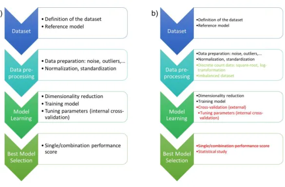
Their need for normalization was formalized based on the definition of a workflow that contains the following phases in order to clearly state where the differences are located within our proposal: dataset, pre-processing of data, learning and selection of the best model, which are graphically represented inFig. 1A. The following paragraphs describe more in depth each of them.
Figure 1 (A) shows the workflow of the experimental design in computational intelligence previously published in the literature and (B) details the phases where methodological changes are proposed to en-sure that the performance of the machine learning models is not biased and that the resulted models are the best.
for each technique as proposed, but also externally, to ensure that the training of the model is not biased or flawed as shown inFig. 1B. There is also a minor consideration about the pre-processing of the data that arise when machine learning models are applied: how to deal with count data and imbalanced datasets.
Dataset
Firstly, the dataset should be generated, defining its particular characteristics. The definition must contain the variables involved in the study and a brief description of each of them to ensure the reproducibility of the tests by external researchers. In order to ensure that the data are representative enough for the particular problem under study, the help of experts is needed to define the cases (i.e., regions of interest for medical imaging or case-control patients).
Data pre-processing
After the generation of the dataset, data are in a raw or pure state. Raw data are often difficult to analyze, thus they usually require a preliminary study or a pre-processing stage. This study will check that there are no data with incomplete information, outliers or noise. In case that some of the aforementioned situations are present in the dataset, different approaches should be applied to avoid them. Only once this process is finished, it is considered that data are ready for analysis. To understand the importance of this step, it is often said that 80% of the effort of a data analysis, is spent compiling data correctly for analysis (Dasu & Johnson, 2003).
Furthermore, the variables typically present different scales or sizes, making them difficult to compare in equality of conditions. Thus, normalization or standardization techniques are required to make data comparable. Both techniques have certainly drawbacks and none is better than the other. Moreover, the dataset should be studied for each particular problem before applying it. For example, if there is an attempt of performing a normalization step and there are outliers in the data (not previously removed), this step will scale useful data to a small interval. This is a non-desirable behavior. After a normalization step, data are scaled in the range [0,1] in case of numeric values. In case a standardization process was performed, data present a zero average value and a standard deviation equal to one, thus they are independent of the unit of measure. Depending of the type of data, there are other well-known approaches to minimize the influence of the values (raising a feature to a power, taking the logarithm, etc.). In the case of discrete count data, the use of the square-root transformation is recommended in order to normalize count data and then log transform them for subsequent analysis (Cuesta et al., 2008). However, recent works have suggested that further studies are necessary in order to choose the best technique to deal with the original data without transformations (O’Hara & Kotze, 2010), rather than the pre-processing of these data.
Another relevant point when using machine learning methods is how to cope with imbalanced datasets. There are mainly two different approaches to deal with those datasets, oversampling (creating synthetic examples from the minority class), as proposed byChawla et al. (2002)and undersampling (removing samples from the majority class) of the data, as proposed bySeiffert et al. (2010)for balancing purposes.
In this work, the NA (Not Available) values and the NZV (near zero variance) features were removed from the datasets at the first stage. Next, a study about the correlation among variables was performed and the correlated variables with a cutoff higher than 0.90 were removed from the dataset. Finally, a standardization phase was applied in order to center and re-scale data, including the output variables, so that they could have a zero mean value and a standard deviation equal to one.
Model mearning
both cases, the results obtained from this reference model will be the ground truth, along with the following experimental design.
Once the reference model is established, it is time to build and test the model intended to be developed in order to provide better solutions. The range of techniques available to solve any problem is usually very high. Some of these techniques are dependent on the field of study, consequently the researcher should review the state-of-the-art in their research field in order to choose the most suitable method.
Some key points arise at this time, such as the need for measuring the performance that should clearly indicate how well the techniques have performed during this training phase. There are different well-known performance scores, such as Area Under Receiver Operating Characteristic (AUROC), accuracy or F-measure in classification problems or Mean Square Error (MSE), RMSE orR2in regression problems. However, sometimes it is necessary to evaluate the performance of the model using an ad-hoc measure. Furthermore, the over-training and over-fitting of those techniques should be avoided in order to ensure that the obtained model provides good results using unknown data. Techniques such as
cross-validation(CV) (McLachlan, Do & Ambroise, 2005) can be useful in this case.
There are two main aims when using CV during the model learning process. Firstly, CV was used to measure the degree of generalization of the model during the training phase, assessing the particular performance of the model and estimating the performance with unknown data. Secondly, using a CV approach, a comparison was performed betweeenvtwo or more algorithms that were trained under the same conditions and with the same dataset. Instead of running our experiments one time only, at least ten runs were performed and ten different initial seeds were used to separate the data for each dataset independently. Thus, as the CV error alone is not adequate as a decision value to compare a set of algorithms, relevant information is available regarding the behaviour of the models to discard bias related to the particular position of the observations within the file data. For each one of the ten runs, each original dataset was separated in ten random splits (75% training and 25% test) and the CV process was performed only with the training data. Once the model was finally trained, they remaining absolutely unknown 25% of the original data were used for validation purposes. However, the key point in this case is that they proposed this cross-validation process was proposed internally and only in order to select the best combination of parameters for each technique.
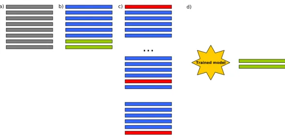
Figure 2 In (A) original data are separated in (B) 75% training and 25% test. A 10-fold cross-validation is run in (C) in order to train the machine learning models, and finally in (D)R2and RMSE are evaluated
with the unknown 25% of the data.
number of featuresAmbroise & McLachlan (2002). The process shown inFig. 2, is repeated ten times for each ML technique/dataset. The final performance measure reported is in this case the average of the values computed for all folds and splits. RMSE,R2and adjustedR2
were computed. Our methodology modified the proposal made byTsiliki et al. (2015a)by adding this external cross-validation step inFig. 2Cin order to ensure that, in each one of the folds, an internal cross-validation was performed to select the best set of parameters as proposed, but no bias or overfitting (model fitting the data) were possible, as independent data were used for validation in each fold.
The RMSE is the square root of the variance of the residuals and has the same units as the response variable. Furthermore, it is an absolute measure that indicates the fit of the model to the data. Finally, this measure is useful to check the ability of the models to predict values for the dependent variable in an absolute sense. The coefficient of determinationR2is in the range from zero to one, the closer the coefficient to one, the better the results. However, this criterion is not appropriate for the comparison of candidate models because overfitting increases artificially its value (Bontempi & Ben Taieb, 2011), as well as the number of features. Finally, this measure is useful to check how well the independent variables explain the variability of the dependent one. The adjusted coefficient of determination incorporates the degrees of freedom of the model in order to avoid the aforementioned problems. It is interpreted as the proportion of total variance, which is explained properly by the model.
Ten linear and non-linear regression models included in the RRegrs package were em-ployed in this work: Multiple Linear Regression (lm) (Kutner, Nachtsheim & Neter, 2004), Generalized Linear Model with Stepwise Feature Selection (glmStepAIC) (Hocking, 1976), Partial Least Squares Regression (PLS) (Wold et al., 1984), Lasso regression (Lasso.RMSE) (Tibshirani, 1994), Elastic Net regression (glmnet) (Zou & Hastie, 2005), Support Vector Machines using radial functions (svmRadial) (Guyon et al., 2002), Neural Networks regres-sion (nnet) (Bishop, 1995), Random Forest (RF) (Breiman, 2001), Random Forest Recursive Feature Elimination (rfRFE) (Saeys, Inza & Larrañaga, 2007) and Support Vector Machines Recursive Feature Elimination (svmRFE) (Dobson & Barnett, 2008). More specifically, glmStepAIC, Lasso.RMSE, svmRFE, rfRFE and glmnet performs dimensionality reduction.
The Supplementary materials include the results of all models with the state-of-the-art and the three real data datasets, as well as the original data files in csv format.
Best model selection
In the previous phase, it has been stated that there were several measures accepted and well known for measuring the performance of a classifier. This does not mean that a researcher is able to compare different classifiers used in the same conditions, using the same dataset with only one run and one error rate. At this point, each technique should be run several times in order to ensure that our results are not biased because of the distribution of the observations within the data or that the number of internal CV runs performed in order to find the best combination of parameters do not bias our results (there is a high probability that a good combination of parameters/performance score is found for a particular distribution of observations when the number of experimental CV runs increases). Consequently, it is a good idea to take into account the mean and standard deviation of all the runs to evaluate the behavior.
With the results obtained by these techniques and in order to determine whether or not the performance of a particular technique is statistically better than that of the others, a null hypothesis test is needed. Furthermore, so that a parametric or a non-parametric test could be used, some required conditions must be checked: independence, normality and heteroscedasticity (García et al., 2010). Note that these assumptions do not refer to the dataset used as input to the techniques, but to the distribution of the performance of the techniques. In statistics, one event is independent of others if the fact that one occurs does not modify the probability of the others. Thus, in computational intelligence, it is obvious that different versions of a set of different algorithms, where initial seeds are used randomly for the separation of data in training and test, comply with the condition of independence. Normality is considered the behavior of an observation that follows a normal or Gaussian distribution; in order to check this condition, there is a different number of tests, such as the Kolmogorov–Smirnov or Shapiro–Wilk (Shapiro & Wilk, 1965). Finally, the violation of the hypothesis of equality of variances, or heteroscedasticity should be checked using, for example, a Levene’s or Bartlett’s tests (Bartlett, 1937).
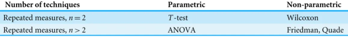
Table 1 The most commonly used parametric and non-parametric statistical tests, according to the num-ber of techniques used in the comparison.
Number of techniques Parametric Non-parametric
Repeated measures,n=2 T-test Wilcoxon Repeated measures,n>2 ANOVA Friedman, Quade
apply aT-test using the performance scores to check if a technique is significantly better than the others. In some cases, this distribution does not met the requirements of this parametric test, consequently a non-parametric test is required. Despite the fact that a parametric test is more powerful a priori, it should not be used when the conditions of independence, normality and homoscedasticity are not fully met. Instead, it is best to employ a non-parametric test, as it was designed specifically for these cases and the result will be more accurate and adjusted to the intrinsic characteristics of the data. Depending on the particular number of techniques that are used in the comparison, a different statistical test should be applied, some of the most common ones being shown inTable 1.
Despite the fact that the Friedman and Quade tests can be used under the same circumstances, in our methodology the use of the Friedman test was proposed with the Iman-Davenport extension as there are ten regression models to be compared and (García et al., 2010) stated that theQuade (1979)test performed better when the number of algorithms was low, at no more than 4 or 5.
Finally, after the null hypothesis test (parametric or non-parametric) was rejected, a
post hoc procedure had to be used in order to address the multiple hypothesis testing and to correct the p-valueswith theadjusted p-values(APV). Among the differentpost hoc
procedures (i.e., Bonferroni-Dunn, Holm, Hochberg, Hommel, Finner, etc.) the Finner procedure was chosen, as it is easy to understand and offers better results than the others, as stated inGarcía et al. (2010).
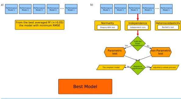
Figure 3Aincludes a comparison between how the previously published methodology selected the best model under a criterion based on the ranking of the best averagedR2and how the best model model was selected with the minimum RMSE from the top ones in the range (±0.05). On the other hand,Fig. 3Bpresents our proposal to select the best model
according to a statistical criterion.
During this last phase, in the event that the results are not statistically significant, the simplest would be chosen from among the models that are winners of the null hypothesis test, either in terms of complexity or runtime. In a more strict sense, one could also perform a new null hypothesis test using only the results of the winning models, but in this case another performance measure should be employed, such as the number of features if a process of feature selection is carried out. Therefore, one could conclude that from among the initially selected winning models, there is a statistically significant difference according to this new second performance criterion (Fernandez-Lozano et al., 2016).
Figure 3 Workflow for the best model selection according to the (A) RRgres methodology and (B) our proposal.
approach proposed inDoksum (1967), which is a contrast estimation based on medians aimed at assessing the real numeric difference between both methodologies.
RESULTS
Preliminary results from UC Irvine Machine Learning repository datasets
Five of the most relevant datasets used for standard regression are used as the starting point to compare the proposed methodology against the previously described inTsiliki et al. (2015a). The selected datasets were: Housing, MachineCPU, WineQuality, Automobile and Parkinson.
Table 2showsR2statistic values for these standard datasets and all the methods available in the package (winning model in bold for RRegrs). All experiments were run with RRegrs version 0.0.5 and following the same conditions as inTsiliki et al. (2015a)with 10 different dataset splits, using 10-fold cross-validation and finally 10 runs with the best model and randomizing the response variable (Y-randomization) in order to ensure that no bias is included in the analysis (Tropsha, 2010).
According to our methodology, the same winning model as in the methodology proposed byTsiliki et al. (2015a)was selected, with the Housing and the Parkinson datasets. Thus, our methodology rejects the best model selected for three out of five datasets: MachineCPU (RF was selected instead of nnet as the best method), WineQuality (rfRFE instead of RF) and Automobile (RF instead of rfRFE). The following paragraphs present the statistical studies that support these differences.
Table 2 RRegs:R2values for UCI Datasets (average for 10 splits).
Housing Machine CPU Wine quality Automobile Parkinson
rfRFE 0.8765 0.8949 0.5008 0.9149 0.9003
RF 0.8744 0.9073 0.5010 0.9159 0.9721
svmRadial 0.8444 0.7655 0.3964 0.8546 0.6370 nnet 0.8349 0.8771 0.3693 0.8036 0.5449 svm-RFE 0.7277 0.6766 0.3796 0.6373 0.4793 glmStepAIC 0.7092 0.8249 0.3528 0.8236 0.1534
lm 0.7075 0.8218 0.3547 0.8237 0.1535
glmnet 0.7061 0.8250 0.3546 0.8279 0.1538 Lasso.RMSE 0.7045 0.8279 0.3538 0.8295 0.1538
PLS 0.6603 0.7932 0.3313 0.7839 0.1214
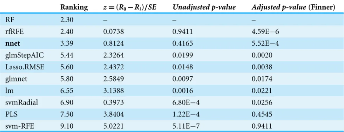
Table 3 Machine CPU dataset results using RF as the control model.
Ranking z=(R0−Ri)/SE Unadjusted p-value Adjusted p-value(Finner)
RF 2.30 – – –
rfRFE 2.40 0.0738 0.9411 4.59E−6
nnet 3.39 0.8124 0.4165 5.52E−4
glmStepAIC 5.44 2.3264 0.0199 0.0020 Lasso.RMSE 5.60 2.4372 0.0148 0.0038
glmnet 5.80 2.5849 0.0097 0.0174
lm 6.55 3.1388 0.0016 0.0221
svmRadial 6.90 0.3973 6.80E−4 0.0256
PLS 7.50 3.8404 1.22E−4 0.4545
svm-RFE 9.10 5.0221 5.11E−7 0.9411
andW of 0.94525. Thus, the null hypothesis was rejected and our results did not follow a normal distribution. A Barlett’s test was performed with the null hypothesis that our results were heteroscedastic. The null hypothesis with ap-valueof 0.01015 and ak-squared
value of 21.623 was rejected. At this point, two conditions are not met; consequently, a non-parametric test should be employed, assuming the null hypothesis that all models have the same performance. The null hypothesis was rejected with the Friedman test and the Iman-Davenport extension (p-value<1.4121E–10). Hence, at this point, the null hypothesis is rejected with a very high level of significance, showing that the winning model is RF.
The average rankings for the Machine CPU dataset, are shown inTable 3. This table also presents for each technique the test statistic of the Friedman test (z), theunadjusted p-valueand theadjusted p-valuewith Finner’s procedure.
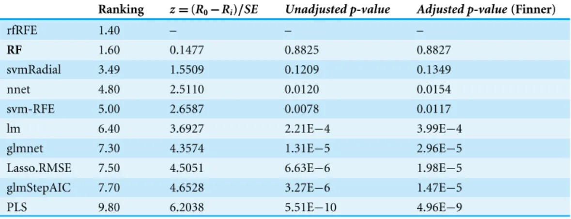
Table 4 Wine Quality dataset results using RF as the control model.
Ranking z=(R0−Ri)/SE Unadjusted p-value Adjusted p-value(Finner)
rfRFE 1.40 – – –
RF 1.60 0.1477 0.8825 0.8827
svmRadial 3.49 1.5509 0.1209 0.1349
nnet 4.80 2.5110 0.0120 0.0154
svm-RFE 5.00 2.6587 0.0078 0.0117 lm 6.40 3.6927 2.21E−4 3.99E−4 glmnet 7.30 4.3574 1.31E−5 2.96E−5 Lasso.RMSE 7.50 4.5051 6.63E−6 1.98E−5 glmStepAIC 7.70 4.6528 3.27E−6 1.47E−5 PLS 9.80 6.2038 5.51E−10 4.96E−9
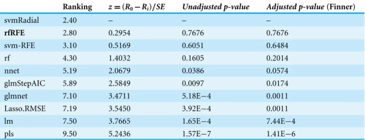
Table 5 Automobile dataset results using RF as the control model.
Ranking z=(R0−Ri)/SE Unadjusted p-value Adjusted p-valueFinner
RF 1.30 – – –
rfRFE 1.70 0.2954 0.7676 0.7676
svmRadial 4.39 2.2895 0.0220 0.0247 Lasso.RMSE 5.10 2.8064 0.0050 0.0064
glmnet 5.20 2.8803 0.0039 0.0059
glmStepAIC 6.10 3.5450 3.92E−4 7.06E−4 lm 6.39 3.7665 1.65E−4 3.72E−4 nnet 7.00 4.2097 2.55E−5 7.67E−5 PLS 8.30 5.1698 2.34E−7 1.05E−6 svmRFE 9.50 6.0561 1.39E−9 1.25E−8
z=(Ri−Rj)
q k(k+1)
6n
. (1)
Secondly, results showed that for 10 different dataset splits, using 10-fold repeated CV for and with the WineQuality dataset, according to a Shapiro–Wilk test with the null hypothesis that the data follow a normal distribution, obtaining ap-valueof 0.0001449 and aW of 0.93794. Thus, the null hypothesis was rejected and our results did not follow a normal distribution. A Barlett’s test was performed with the null hypothesis that our results were heteroscedastic. The null hypothesis with ap-valueof 0.9903 and ak-squared
Table 6 Corona dataset results using RF as the control model.
Ranking z=(R0−Ri)/SE Unadjusted p-value Adjusted p-value(Finner)
RF 3.30 – – –
Lasso.RMSE 3.39 0.0738 0.9411 0.9411
pls 3.99 0.5169 0.6051 0.6973
glmnet 4.00 0.5169 0.6051 0.6973
svm-RFE 5.00 1.2555 0.2092 0.2968
rfRFE 5.30 1.4470 0.1396 0.2871
svmRadial 5.30 1.4770 0.1396 0.2871
nnet 5.89 1.9202 0.0548 0.1556
lm 9.39 4.5051 6.63E−6 5.96E−5 glmStepAIC 9.39 4.5051 6.63E−6 5.96E−5
Table 7 Metal oxides dataset results using glmnet as the control model.
Ranking z=(R0−Ri)/SE Unadjusted p-value Adjusted p-value(Finner)
glmnet 2.80 – – –
nnet 2.99 0.1825 0.8551 0.8551
pls 3.40 0.5477 0.5838 0.7069
Lasso.RMSE 3.40 0.5477 0.5838 0.7069 svmRadial 4.60 1.6431 0.1003 0.1689
rf 5.20 2.1908 0.0284 0.0651
lm 6.80 3.6514 2.60E−4 0.0018
glmStepAIC 6.80 3.6514 2.60E−4 0.0018
Table 8 Toxicity dataset results using svmRadial as the control model.
Ranking z=(R0−Ri)/SE Unadjusted p-value Adjusted p-value(Finner)
svmRadial 2.40 – – –
rfRFE 2.80 0.2954 0.7676 0.7676
svm-RFE 3.10 0.5169 0.6051 0.6484
rf 4.30 1.4032 0.1605 0.2014
nnet 5.19 2.0679 0.0386 0.0574
glmStepAIC 5.89 2.5849 0.0097 0.0174 glmnet 7.10 3.4711 5.18E−4 0.0011 Lasso.RMSE 7.19 3.5450 3.92E−4 0.0011 lm 7.50 3.7665 1.65E−4 7.44E−4 pls 9.50 5.2436 1.57E−7 1.41E−6
As in the previous case,Table 4shows the average rankings of the techniques compared for the Wine Quality dataset. The ranking was presented, as well as each technique in the comparison with the test statistic of the Friedman test (z), theunadjusted p-valueand the
adjusted p-valuewith Finner’s procedure.
data follow a normal distribution obtained ap-valueof 3.375E–10 andWof 0.80435. Thus, the null hypothesis was rejected and our results did not follow a normal distribution. A Barlett’s test was performed with the null hypothesis that our results were heteroscedastic. The null hypothesis with ap-valueof 3.683E–08 and ak-squaredvalue of 52.47 was rejected. At this point, two conditions are not met; consequently, a non-parametric test should be employed assuming the null hypothesis that all models have the same performance. The null hypothesis was rejected with the Friedman test and the Iman-Davenport extension (p-value<5.031E–20). Hence, at this point the null hypothesis is rejected with a very high level of significance, showing that the winning model is RF.
The average rankings of the techniques compared for the Automobile dataset, and the test statistic of the Friedman test (z), theunadjusted p-valueand theadjusted p-valuewith Finner’s procedure are shown inTable 5.
Cheminformatics use case modeling
Once the proposed methodology provided satisfactory results using simple and well-known state-of-the-art datasets, it is tested against more complex problems. InTsiliki et al. (2015a)authors proposed three case studies to test a methodology related to computer-aided model selection for QSAR predictive modelling in cheminformatics: proteomics data for surface-modified gold nanoparticles (Corona dataset), nano-metal oxides descriptor data (Gajewicz dataset), and molecular descriptors for acute aquatic toxicity data (Toxicity dataset).
Protein corona case study
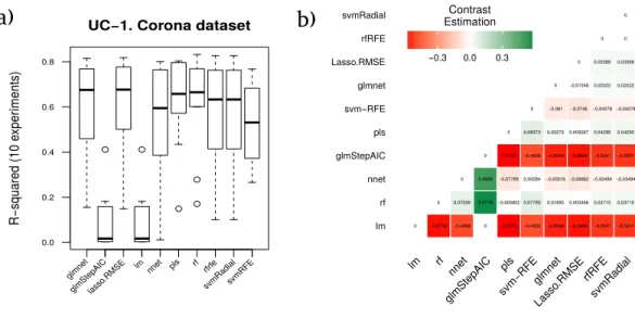
Recent studies have shown that the presence of serum proteinsin vitrocell culture systems form a protein adsorption layer (a.k.a. the ‘protein corona’) on the surface of nanoparticles (NPs). This section presents the results for the recently published proteomics data that characterizes the serum protein corona ‘fingerprint’ formed around a library of 105 distinct surface-modified gold NPs (Walkey et al., 2014). The authors used LC-MS/MS to identify 129 serum proteins which were considered suitable for relative quantification. From this dataset, the methodology proposed on RRegrs establishes that the best regression algorithm is svmRadial (with an average ofR2: 0.5758) for this dataset.
However, the statistical study included as one of the required steps in the proposed methodology stated that the best model (in terms of accuracy and stability of results) should be RF (with an averageR2of 0.6191), giving the seventh position to svmRadial. The
average rankings of the techniques compared for the use case 1 (methodology application on protein corona data), are shown inTable 6. This table also presents for each technique the comparison between the test statistic of the Friedman test (z), theunadjusted p-value
and theadjusted p-valuewith Finner’s procedure. The name of the best model according to the methodology proposed in RRegrs is shown in bold.
Figure 4 Results for the corona dataset.(A) Boxplot for the ten runs of each technique in order to show the behavior and stability of the method. (B) Contrast estimation based on medians where a positive dif-ference value indicates that the method performs better than the other (green color).
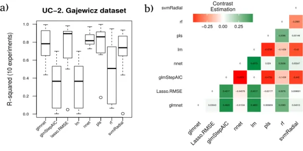
Gajewicz metal oxides case study
The authors ofGajewicz et al. (2015)combined experimental and theoretical measurements to develop a nano-QSAR model that described the toxicity of eighteen nano-metal oxides (MeOx) to the human keratinocyte (HaCaT) cell line, which is a commonin vitromodel for keratinocyte response during toxic dermal exposure. They calculated 32 parameters for each of the 18 samples that quantitatively describe the variability of the nanoparticles’ structure, called nano-descriptors, including particle size and size distribution, agglomeration state, particle shape, crystal structure, chemical composition, surface area, surface chemistry, surface charge, electronic properties (reactivity, conductivity, interaction energies, etc.), and porosity.
In this case, Table 7shows the average rankings of the techniques compared for this dataset and the test statistic of the Friedman test (z), theunadjusted p-valueand theadjusted p-valuewith Finner’s procedure for each technique within the comparison.
The best model according to the RRegrs methodology (pls, in bold inTable 7) achieves an averageR2of 0.7885 whereas a more in depth analytical study of results provides glmnet as the best method with an averageR2of 0.7684. This is due to the higher stability of the results during the ten experiments provided by glmnet against the results achieved by PLS as shown inFig. 5A).
The average performanceR2corresponding to each technique for the ten runs is shown in Fig. 5A, as well as the contrast estimation based on medians between the different approaches inFig. 5B.
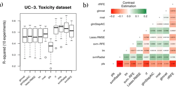
Aquatic toxicity case study
Figure 5 Results for the Gajewicz dataset.(A) Boxplot for the ten runs of each technique in order to show the behavior and stability of the method. (B) Contrast estimation based on medians where a positive difference value indicates that the method performs better than the other (green color).
for short-term aquatic toxicity testing. The data set provided 546 organic molecules and a set of 201 descriptors which were used to perform the classification.
The average rankings of the techniques on aquatic toxicity data are shown inTable 8. This table also presents for each method the statistic value of the Friedman test (z), the
unadjusted p-valueand theadjusted p-valuewith Finner’s procedure. The name of the best model according to the RRegrs methodology is in bold.
In this last dataset, the best model according to RRegrs was rfRFE which achieved an averageR2of 0.5255. The methodology proposed in our manuscript establishes svmRadial
as the most reliable model in terms of stability and accuracy of the results, with an R2
of 0.5365.
The averaged performanceR2 corresponding to each technique for the ten runs is shown inFig. 6A, as well as the contrast estimation based on medians between the different approaches inFig. 6B.
DISCUSSION
Figure 6 Results for the toxicity dataset.(A) Boxplot for the ten runs of each technique in order to show the behavior and stability of the method. (B) Contrast estimation based on medians where a positive dif-ference value indicates that the method performs better than the other (green color).
the quality of the image analysis of proteins separated on a gel (Fernandez-Lozano et al., 2016). These works were based on the experience of the group obtained in the processing of several cheminformatics datasets related to classification tasks (Fernandez-Lozano et al., 2013;Fernandez-Lozano et al., 2014;Aguiar-Pulido et al., 2013).
In the present work, the same methodology for the formalization of experimental designs was proven over a dataset related to regression tasks. These tests include simple datasets from the UCI Machine Learning repository and more complex case studies for QSAR predictive modeling. The achieved results show an excellent performance of the final selected models and demonstrate the importance of taking into account the variability of the models in order to choose the best one. This selection should not be based only on the best result achieved in one execution or in terms of the previously published methodology. The authors evaluated the performance of all models (with the test set) according toR2and established a ranking. In the next step, they took into consideration all the models which are in the range (±0.05) according to this measure, and reordered the ranking, choosing
the one with the lowest RMSE obtained in test.
The results also allowed us to understand that selecting the model only according to the best R2or the highest accuracy and taking into consideration only one run is not stastically valid. An unusual high value in performance can be an outlier or maybe be due to a particular partition of the data during the model learning and should be discarded in favor of more stable methods. Aspects like stability in the results should be taken into account to make this selection.
our knowledge, our findings are of relevance and it can be assumed that other Machine Learning models, in general, should behave similarly to those presented in this work, as well as the same algorithms with other datasets. Generally speaking, if the training process or the algorithms are stochastic in some way, one should repeat several experimental runs in order to find the best results, and it is crucial to use a statistical comparison to evaluate whether the differences in performance score are relevant before assuming a final best model. Otherwise, the final conclusions could be wrong and the final model should be discarded.
Furthermore, in order to ensure the power and validity of our results and methodology, using the data resulting from the different splits over the three cheminformatics use cases datasets, the estimation of the differences between each pair of ML techniques was checked, using the approach proposed inDoksum (1967)as shown inFigs. 4–6B. Thus, the real differences between our methodology and the one proposed in RRgres (Tsiliki et al., 2015a) could be computed. This procedure is especially useful to estimate a method’s performance over another (García et al., 2010).
Finally, it was proven that our methodology is applicable in other fields, as it is enough open to add new phases and we test our proposal with eight different datasets from very different scopes. At the same time, given our results, it can be stated that the same behavior is expected with other ML algorithms and further statistical studies are expected to be relevant in this sense.
The main objective of this kind of methodologies in QSAR predictive modeling is to help with the initial exploration of extensive databases of drugs, proteins, molecules, etc. in order to design comprehensivein silicoscreening methods, reducing the economic costs as much as possible. At the same time, the quality and reliability of the ML methods used in the process should be ensured.
CONCLUSIONS
This paper proposed a new multidisciplinary methodology for performing experiments in Computational Intelligence, which was tested with a well-known methodology in the area using the RRegrs package. Ten computational intelligence algorithms for data mining regression tasks and five state-of-the-art datasets were used in this sense. Different critical modifications were proposed and tested in several phases of the previous published methodology, and our results are of relevance. For a better understanding of our proposal, all the steps were applied to the baseline example of an experimental study on well-known state-of-the-art datasets previously published in different fields.
against poorly experimental designs in order to clearly state that the obtained results are stable, reproducible and relevant.
In the near future, our group is planning to include this methodology in the RRegrs package so that it could be used by the scientific community, as this work is distributed under the terms of the Creative Commons Attribution 4.0 International License.
ACKNOWLEDGEMENTS
The authors would like to thank the Overleaf team for their support with the template during the writing of our manuscript, especially Dr. Lian Tze Lim and Dr. John Hammersley.
ADDITIONAL INFORMATION AND DECLARATIONS
Funding
This study was supported by the Galician Network of Drugs R+D REGID (Xunta de Galicia R2014/025), by the General Directorate of Culture, Education and University Management of Xunta de Galicia (Ref. GRC2014/049) and by ‘‘Collaborative Project on Medical Informatics (CIMED)’’ PI13/00280 funded by the Carlos III Health Institute from the Spanish National plan for Scientific and Technical Research and Innovation 2013–2016 and the European Regional Development Funds (FEDER) and the Juan de la Cierva fellowship programme by the Spanish Ministry of Education (Carlos Fernandez-Lozano, Ref. FJCI-2015-26071). The funders had no role in study design, data collection and analysis, decision to publish, or preparation of the manuscript.
Grant Disclosures
The following grant information was disclosed by the authors: Galician Network of Drugs R+D REGID: R2014/025.
General Directorate of Culture, Education and University Management of Xunta de Galicia: GRC2014/049.
Collaborative Project on Medical Informatics (CIMED): PI13/00280. Carlos III Health Institute from the Spanish National plan for Scientific. Technical Research and Innovation 2013–2016.
European Regional Development Funds (FEDER).
Juan de la Cierva fellowship programme by the Spanish Ministry of Education: FJCI-2015-26071.
Competing Interests
The authors declare there are no competing interests.
Author Contributions
• Carlos Fernandez-Lozano and Marcos Gestal conceived and designed the experiments,
performed the experiments, analyzed the data, contributed reagents/materials/analysis tools, wrote the paper, prepared figures and/or tables, reviewed drafts of the paper.
• Julian Dorado conceived and designed the experiments, analyzed the data, reviewed
drafts of the paper.
• Alejandro Pazos conceived and designed the experiments, contributed
reagents/materi-als/analysis tools, reviewed drafts of the paper.
Data Availability
The following information was supplied regarding data availability: The raw data has been supplied as aData S1.
Supplemental Information
Supplemental information for this article can be found online athttp://dx.doi.org/10.7717/ peerj.2721#supplemental-information.
REFERENCES
Aguiar-Pulido V, Seoane JA, Gestal M, Dorado J. 2013.Exploring patterns of epige-netic information with data mining techniques.Current Pharmaceutical Design
19(4):779–789DOI 10.2174/138161213804581936.
Ambroise C, McLachlan GJ. 2002.Selection bias in gene extraction on the basis of microarray gene-expression data.Proceedings of the National Academy of Sciences of the United States of America99(10):6562–6566DOI 10.1073/pnas.102102699.
Baker M. 2016a.1,500 scientists lift the lid on reproducibility.Nature533:452–454
DOI 10.1038/533452a.
Baker M. 2016b.Reproducibility: seek out stronger science.Nature537:703–704
DOI 10.1038/nj7622-703a.
Bartlett MS. 1937.Properties of sufficiency and statistical tests.Proceedings of the Royal Society of London. Series A, Mathematical and Physical Sciences160(901):268–282
DOI 10.1098/rspa.1937.0109.
Bishop CM. 1995. Neural networks for pattern recognition. Cambridge: Oxford University Press.
Bontempi G, Ben Taieb S. 2011.Statistical foundations of machine learning. Brussells: Université Libre de Bruxelles. Available athttps:// www.otexts.org/ book/ sfml.
Breiman L. 2001.Random forests.Machine Learning 45(1):5–32
DOI 10.1023/A:1010933404324.
Cassotti M, Ballabio D, Consonni V, Mauri A, Tetko I, Todeschini R. 2014.Prediction of acute aquatic toxicity toward Daphnia magna by using the GA-kNN method.
Alternatives to Laboratory Animals: ATLA42(1):31–41.
Chawla NV, Bowyer KW, Hall LO, Kegelmeyer WP. 2002.SMOTE: synthetic minority over-sampling technique.Journal of Artificial Intelligence Research16(1):321–357.
Cuesta D, Taboada A, Calvo L, Salgado J. 2008.Short- and medium-term effects of experimental nitrogen fertilization on arthropods associated with Calluna vulgaris heathlands in north-west Spain.Environmental Pollution152(2):394 – 402
Daniel W. 1990.Applied Nonparametric Statistics. Pacific Grove: Duxbury Thomson Learning.
Dasu T, Johnson T. 2003. Exploratory data mining and data cleaning. Vol. 479. Hobo-ken: John Wiley & Sons.
Dobson AJ, Barnett A. 2008. An introduction to generalized linear models. Boca Raton: CRC press.
Doksum K. 1967.Robust procedures for some linear models with one observation per cell.Annals of Mathematical Statistics38(3):878–883DOI 10.1214/aoms/1177698881.
Donoho DL. 2000.High-dimensional data analysis: the curses and blessings of dimen-sionality. In:Mathematical challenges of the 21st century conference of the American Mathematical Society. Los Angeles: American Mathematical Society,Available at
http:// www-stat.stanford.edu/ ~donoho/ Lectures/ AMS2000/ AMS2000.html.
Fernandez-Lozano C, Gestal M, González-Díaz H, Dorado J, Pazos A, Munteanu CR. 2014.Markov mean properties for cell death-related protein classification.Journal of Theoretical Biology349:12–21DOI 10.1016/j.jtbi.2014.01.033.
Fernandez-Lozano C, Gestal M, Pedreira-Souto N, Postelnicu L, Dorado J, Robert Munteanu C. 2013.Kernel-based feature selection techniques for transport proteins based on star graph topological indices.Current Topics in Medicinal Chemistry
13(14):1681–1691DOI 10.2174/15680266113139990119.
Fernandez-Lozano C, Seoane JA, Gestal M, Gaunt TR, Dorado J, Campbell C. 2015.
Texture classification using feature selection and kernel-based techniques.Soft Computing 19(9):2469–2480DOI 10.1007/s00500-014-1573-5.
Fernandez-Lozano C, Seoane JA, Gestal M, Gaunt TR, Dorado J, Pazos A, Campbell C. 2016.Texture analysis in gel electrophoresis images using an integrative kernel-based approach.Scientific Reports6:19256DOI 10.1038/srep19256.
Fourches D, Muratov E, Tropsha A. 2010.Trust, but verify: on the importance of chem-ical structure curation in cheminformatics and QSAR modeling research.Journal of Chemical Information and Modeling 50(7):1189–1204DOI 10.1021/ci100176x.
Gajewicz A, Schaeublin N, Rasulev B, Hussain S, Leszczynska D, Puzyn T, Leszczynski J. 2015.Towards understanding mechanisms governing cytotoxicity of metal oxides nanoparticles: hints from nano-QSAR studies.Nanotoxicology9(3):313–325
DOI 10.3109/17435390.2014.9301950.
García S, Fernández A, Luengo J, Herrera F. 2010.Advanced nonparametric tests for multiple comparisons in the design of experiments in computational intel-ligence and data mining: experimental analysis of power.Information Sciences
180(10):2044–2064DOI 10.1016/j.ins.2009.12.010.
Gilad Y, Nadassy K, Senderowitz H. 2015.A reliable computational workflow for the selection of optimal screening libraries.Journal of Cheminformatics7(1):1–17
DOI 10.1186/s13321-015-0108-0.
Guyon I, Weston J, Barnhill S, Vapnik V. 2002.Gene selection for cancer classi-fication using support vector machines.Machine Learning46(1–3):389–422
Hocking RR. 1976.A Biometrics invited paper. The analysis and selection of variables in linear regression.Biometrics32(1):1–49DOI 10.2307/2529336.
Kutner MH, Nachtsheim C, Neter J. 2004.Applied linear regression models. New York: McGraw-Hill/Irwin.
Lichman M. 2015.UCI machine learning repository, 2013.Available athttp:// archive. ics. uci. edu/ ml, 114.
McLachlan G, Do K-A, Ambroise C. 2005. Analyzing microarray gene expression data. Vol. 422. Hoboken: John Wiley & Sons.
O’Hara RB, Kotze DJ. 2010.Do not log-transform count data.Methods in Ecology and Evolution1(2):118–122DOI 10.1111/j.2041-210X.2010.00021.x.
Quade D. 1979.Using weighted rankings in the analysis of complete blocks with additive block effects.Journal of the American Statistical Association74(367):680–683
DOI 10.1080/01621459.1979.10481670.
Saeys Y, Inza IN, Larrañaga P. 2007.A review of feature selection techniques in bioinfor-matics.Bioinformatics23(19):2507–2517DOI 10.1093/bioinformatics/btm344.
Seiffert C, Khoshgoftaar TM, Hulse JV, Napolitano A. 2010.RUSBoost: a hybrid approach to alleviating class imbalance.IEEE Transactions on Systems, Man, and Cybernetics - Part A: Systems and Humans40(1):185–197
DOI 10.1109/TSMCA.2009.2029559.
Shapiro SS, Wilk MB. 1965.An analysis of variance test for normality (complete samples).Biometrika52(3–4):591–611DOI 10.1093/biomet/52.3-4.591.
Tibshirani R. 1994.Regression selection and shrinkage via the lasso.Journal of the Royal Statistical Society: Series B (Statistical Methodology)58:267–288.
Tropsha A. 2010.Best practices for QSAR model development, validation, and exploita-tion.Molecular Informatics29:476–488DOI 10.1002/minf.201000061.
Tsiliki G, Munteanu CR, Seoane JA, Fernandez-Lozano C, Sarimveis H, Willighagen EL. 2015a.RRegrs: an R package for computer-aided model selection with multiple regression models.Journal of Cheminformatics7:1–16
DOI 10.1186/s13321-015-0094-2.
Tsiliki G, Munteanu CR, Seoane JA, Fernandez-Lozano C, Sarimveis H, Willighagen EL. 2015b. Using the RRegrs R package for automating predictive modelling. In:
MOL2NET, international conference on multidisciplinary sciences.
Walkey CD, Olsen JB, Song F, Liu R, Guo H, Olsen DWH, Cohen Y, Emili A, Chan WCW. 2014.Protein corona fingerprinting predicts the cellular interaction of gold and silver nanoparticles.ACS Nano8(3):2439–2455DOI 10.1021/nn406018q.
Wold S, Ruhe A, Wold H, Dunn III W. 1984.The collinearity problem in linear regres-sion. The partial least squares (PLS) approach to generalized inverses.SIAM Journal on Scientific and Statistical Computing 5(3):735–743 DOI 10.1137/0905052.
Zou H, Hastie T. 2005.Regularization and variable selection via the elastic net.Journal of the Royal Statistical Society: Series B (Statistical Methodology)67(2):301–320