Todos os direitos reservados.
É proibida a reprodução parcial ou integral do conteúdo
deste documento por qualquer meio de distribuição, digital ou
impresso, sem a expressa autorização do
REAP ou de seu autor.
Incentive theory for the transition from Atlantic
slave plantations to firms and labor markets
Steve De Castro
to firms and labor markets
Steve De Castro
Steve De Castro#
Former professor University of Brasília Dept of Economics e-mail:
stevedecas@gmail.com
Model extracted and clarity-enhanced in December 2015, from the original:
“Wrong incentives for growth in the transition from modern slavery* to firms and labor
markets: Babylon before, Babylon af
ter”,
Social & Economic Studies
53(2) June, 2004.
Full text of the paper is available on line in S&ES, distributed by Proquest Periodicals.
See also De Castro [2005] in Portuguese, but without the model.
And De Castro [2001], an early version of the model:
http://epge.fgv.br/files/1049.pdf
.
AbstractThe reallocation of property rights at the transition from slavery to free labor in Brazil, the US South, Jamaica, among others, were often followed by stagnation and even falls in GDP per capita. One theory for the higher productivity of slaves claims it was the coercion available to slave-owners and not to employers. A second argues that plantations were using various incentives to induce it – more food, time-off etc. Loss of scale at abolition is the implied theory. In this paper, some recent theories of the firm are used to study the incentive mechanisms when effort at multiple tasks must be supervised. A principal-agent model is used to show how wrong incentives after abolition could have induced former slaves to produce more peasant crops relative to the plantation staples which yielded more GDP. If at the transition to free workers there is no technical progress or changes in product prices, plantations may become unviable and the economy can collapse into
lower-productivity family farms or worse. An exception to this argument is the “gold rush” outcome
where the pulverized activity is so lucrative that growth can occur without hierarchical production structures. In the absence of such windfalls, agents may resort to less efficient, incentive-compatible mechanisms akin to sharecropping, tenancy and marginal-product wage labor which do not need the supervision which firms provide.
Key words: Firms, labor markets, property rights, incentives, slave plantations. JEL classes: D21, D23, J41, N30
__________________________________________________
*Ancient slavery is the case where the master offers no cooperating skills in a joint effort at production. The master’s share would be coercive, like a tax. The analysis of this case was done by Evsey Domar [1970], in economies with only labor and land, and constant returns. If land is in surplus relative to labor, no one will choose freely to work for someone else. For a rentier class of agents to emerge here, either access to land must be blocked, serfdom, or labor must be coerced, slavery. Labor productivity must of course be above subsistence.
___________________________________________________
The transition from slave plantations to firms and labor markets
1. The historical background
The passage from slavery to labor markets was followed by falls in the average income per
person of most regions of the Atlantic economy which used this mode, despite exploding demand
for their products. In the reallocation of property rights at abolition, both ex-slaves and ex-masters
lost, as incomes in the US south, Brazil, Jamaica, among others, fell behind regions outside the
slave belt which began to grow rapidly with free migrant workers, in the same decades before 1914
during which the US north made the US the richest country in the world (see GDP per capita table
in Appendix C). Brazil’s GDPpc in 1913, for example, was less than it was in 1850. Jamaica took nearly 100 years to return to its level of 1832, 2 years before abolition, and is the inspiration for the
“Babylon after” in the title of the original S&ES paper. Only one has caught up with the rich regions despite some with high growth rates over many decades of the 20th century.
For us, the distinguishing feature of modern slavery is the perception by masters, mainly in
the Americas and from around the same time as the first industrial revolution, that they could obtain
more income from their slaves by offering both incentives and some complementary input in the
core activities of the plantation. This was the fundamental contribution of Fogel & Engerman’s 1974 book, Time on the cross, which caused a furious debate among US economic historians (see
especially Paul A. David et al [1976, 1979]) some of whom contested, unsuccessfully in our view
and Barzel’s [1977], their finding that the imputed real income of a slave on large plantations (>15 slaves) in the US cotton belt around 1860, was more than that of a free small farmer in the same
region. To explain why these folk did not offer to compete with slaves despite their lower incomes,
Fogel & Engerman attributed the difference to the psychic income derived from being free men.
Barzel’s interpretation of the extra food, time-off etc is that they were the biological complements of the forced labor regime, with no incentive component. We shall contest both these theories.
Unlike Barzel, we claim that it is not necessary to know whether, under slavery, an
incentive component was present or not, or even whether the plantation offered no expertise or
managerial ability but just physical punishment or the threat of it. Once the data on the higher
productivity of slaves are accepted as true, a crucial step in the debate, one can use economic theory
to check whether a free labor regime can reproduce it or not. The extra output is available for
creating incentives to induce free agents to accept the discipline required of supervised employees,
so that the re-distribution of incomes at abolition need not be the inferior Nash equilibrium, the
Eisenberg’s work on the dominant sugar industry in Pernambuco, Northeast Brazil, 1840-1910 [1974 p.213-4] gives the clue to our theoretical argument for the link between the role of
supervision and the fall in incomes:
“after the early 1870s, the wage rate fell steadily. All three types of free labor (squatters, sharecroppers, and wage workers) could be hired and fired at will, without complications
of contract or indemnizations …. one cannot escape the conclusion that in the later 19th century, they enjoyed little material advantage over the slave”.
Slavery was still legal then but the Northeast sugar planters were increasingly selling theirs to the
coffee planters in Sao Paulo. He noted further that the apparently “better” treatment of slaves may well have been the source of Gilberto Freyre’s polemical thesis on the paternalism of the Northeast’s slave masters. Our model can explain this without resort to altruism as in Freyre, or to economies of scale as in Fogel & Engerman, but as the reward for taking orders which, like in a
firm, is justified by the gains to both parties from supervision of one by the other. With the
technology of the time, it was probably the economics of supervision which needed scale rather
than the other way round.
Under slavery, however, coercion can never be dismissed entirely. Or to put it in the
language of the model, since slaves did not have the right to quit, it is likely that plantations paid
them less than if they did, even if, as Fogel & Engerman claimed, they paid them more than free
small farmers earned in the same region. The problem we will try to solve is why after abolition,
free workers did not reproduce the higher productivity.
During slavery, free workers seeking a spot wage would not be hired even though their
intrinsic skills may be identical to that of a slave, because the wage regime would not be able to
offer efficient incentives when effort at multiple tasks must be coordinated in complex ways. Thus
we have a better explanation than Fogel & Engerman’s psychic income theory. We shall see that under slavery, a free worker would need to be offered more than a slave to induce him to accept the
discipline of the plantation, provided the slave´s right to quit had positive value. Thus, supervisory
and incentive schemes cannot be the same for free workers, even if under slavery, legal sanctions
against the use of violence existed and were effective.
At abolition, we will show, the plantation would have to change its incentive scheme. It will
not necessarily be worse off because it will no longer have to pay out the capital rentals of the slave
contract. It does not have to buy its workers. In fact, slavery would be redundant if these rents were
greater than any potential reduction in its gross income at abolition, either due to higher worker
These remarks will become clearer after we formalize the ideas below but a bit of
elementary microeconomics may help now. Figure 1 in Appendix C shows the 4 institutions of
modern capitalism, the 3 markets as circles, for labor, capital and product, and the hierarchical firm
as a triangle. In fact, as it stands the figure is contradictory. All 4 cannot coexist in any given
industry. This follows from the Euler theorem as applied to a production function with constant
returns to scale, a property necessary in the neighborhood of minimum long-run average cost for a
competitive equilibrium to exist. For example, if all 3 markets are functioning, factors will receive
their marginal products and their cost will exhaust the revenue of the firm at the competitive price
for the product. The hierarchical firm will have no economic role. All the incentives will be in the
markets. In business school language, the firm has no slack with which to create its own incentives.
Solow’s growth theory was based on this microeconomics, a fact which made it almost surely out-of-date some 50 years before its publication. Another 30 years were needed for the
paradigm shift to market power as the engine. For in modern capitalism, the product market is
usually sacrificed to yield monopoly profits for the hierarchical firm’s incentives. Under modern slavery, it was the labor market, since plantations faced competition for their products, and
ownership of slaves could be financed in capital markets. In Soviet Russia, all 3 markets were
sacrificed, even labor. The Bolsheviks believed that hierarchical enterprises could have provided all
the incentives. So we see that under slavery, the absence of a labor market would have allowed the
slack for the plantations to create incentives for the supervision which generated the higher
productivity. Like modern oligopolies, plantations may have used some of their super-profits for
incentives to their slaves, throwing up the polemical data Fogel & Engerman encountered.
2. A model for the transition
The model uses some recent theories of the firm based on incentives and power (for a
survey see Holmstrom [1999]) to study this failure of the Coase doctrine that, in the absence of
transaction costs, property rights determine only the distribution but not total income. It shows how
wrong incentives at abolition can induce inefficient choices, in levels, of 2 activities. One can be
carried out by a single agent, working alone. The other activity requires a second complementary,
cooperating type 2 agent for its execution. Neither activity needs physical capital. When done
outside the plantation, the first is a stylized version of a single-family, small farm. It is not
necessarily confined to subsistence crops. For example in Jamaica such farms even today grow
bananas for export. In late 19th century Brazil, many raised cattle and planted food crops for local
markets. The second activity, combined with the skill and effort of the type 2 agent, the master, is
What is important here is that we assume that the incentives for the effort at the two
activities by the type 1 agent is better designed by the type 2 who made the fixed investment up
front. However, even under slavery, he must offer suitable incentives to induce effort levels that are
an effective combination with the complementary inputs of the plantation. Asymmetric information
is not explicit in this simplified model, but it is crucial to the argument. The issue can be understood
if, unlike here in our simplified model, one supposed there were increasing returns to labor in the
plantation staple. With increasing returns, the notion that individual effort is observable by an
outside party (verifiable) becomes tenuous.
2.1 The general framework
There are two products y1, y2both of which are sold on markets at perfectly competitive
prices p1, p2.Later, we shall simplify the model by using
2 1
p
p
p
, the relative price. y1 is thegood the slave or free worker can produce without the inputs of the plantation, his kitchen garden
crop, and y2 is the plantation staple.
There are two types of agents:
Type 1: can exert effort at two different activities, e1 ,e2. At activity 1, an effort level e1
produces
y
1
R
e
1,
R
e
1
0
,
R
e
1
0
, without need of the second type of agent’s input. At activity 2, an effort level e2 produces y2 = e2, provided the complementary skills of a type 2 agentare joined. Activity 1 is the type 1’s garden crop, while activity 2 yields the plantation staple. Under slavery, type 1 agents will be the slaves.
Type 2: have special skills (marketing, production know-how, coordination) or other inputs
(e.g. equipment) which are complementary to type 1 agents’ effort e2 at producing y2. For
simplicity, assume fixed proportions and linearity (crs) in the effort levels of the two types. We will
assume that it is the type 2 agent who makes the irreversible investment (in equipment, acquiring
skills etc). All these can be subsumed under the rubric of his effort level which he will set first, and
then design an incentive scheme to induce the type 1 to choose the correct effort level e2 for activity
2, the plantation staple. The same scheme may induce different reactions by the type 1 agents
depending on whether they are slaves or free workers.
We will focus initially on the type 1 agent’s incentives and decisions to allocate effort levels e1, e2 between the two tasks, which we assume to be equally disagreeable to him, and
non-separable in their disutility. We will show later that the functional form chosen now for disutility of
his effort is such that if at abolition there is no change of incentives, he will exert the same total
Type 1 agent’s utility:
2 2 1 2 2 1 1 } , { 2 1 2 1 e e e e R U Max ee
subject to
e e
1,
2
0
The property rights regime and incentive scheme will determine the values of
1,
2, the share of the revenue from the two goods accruing to this agent.Given
1,
2, and assuming that the non-negativity constraints are not binding, his chosen effort levels will be determined by:
1 1 1 2 1 1
2 2 1
, 0, 0
R e e e R e R e
e e
...(1)
We will now study firstly, how the slavery regime would determine the output mix, and
then how this would change if, at abolition, the plantation did not modify its incentive scheme.
Specifically, we will show that if it didn’t, the freed slave would want to produce more of y1and
less of y2. If the prices of the two products are such that the increased output of the garden crop, y1,
does not compensate in value for the decrease in the plantation staple, then there will be a fall in
GDP at abolition even though the ex-slave’s income may rise, provided the plantation does not modify its incentive scheme or abandon the activity altogether. Finally, we will show how the
plantation can modify its incentives in a way that they both benefit. In the new schemes, it will be
operating like a firm in that it must satisfy the participation constraint of its workers, but will use
supervision instead of an incentive compatible contract to induce an efficient allocation of effort.
Two regimes are studied, slavery and abolition:
1. Slavery: if the type 1 agent is the slave of the type 2,
1,
2 are the latter’s incentives tohim. The type 2 agent will maximize his share of the output by choosing
1,
2 so as to induce the correct effort levels e1, e2 by the type 1. Because of his fixed investment up front, he will want toinduce the slave to allocate more effort to the cooperative activity. Slavery, we assume, allows the
type 2 the power to limit in some way the slave’s activity 1. In practice, this can mean, for example,
an order not to work in his kitchen garden until say Saturday after midday.
We formalize this power of the master by
, the share of the revenue of the 2 activities theslave is allowed to keep. The master will set:
1
p
1;
2p
2; 0
1;
.The slave will then choose:
2 1
1
2 2 1
S
S S
p R e
p
e p e
The rationale for this scheme lies firstly in the fact that his effort levels will depend not only
on
but on the regime. Secondly, increases in
will induce the slave to increase his total effortbut all the extra will go to the plantation staple (see figure 1 below). Thirdly, as we shall see, the
slave will always produce less of his garden crop and allocate more of the same total effort to the
plantation staple than a free worker. If it weren’t for the lack of the right to quit and the threat of violence, this arrangement is similar to those in modern hierarchical firms.
Given the product prices, the level of can be chosen by the master to maximize his profit.
Since in theory he does not have to satisfy the participation constraint of his slave, this is a strong
assumption as it may lead to various forms of resistance and even flight. Under slavery therefore,
some masters may well have respected the constraint. In any case, whatever may be the under
slavery, we shall assume that it is not enough to induce the slave to continue to accept the discipline
of the plantation. Put another way, we want to assume that at abolition, the right to quit had positive
value to the slave and we shall show how to calculate it (see Section 2.4).
2. Free workers at abolition with no change of incentives:
If the type 1 agent is now a free worker,
1
p
1 because he can keep all they
1 revenue,since for this activity he does not need the type 2 agent’s skills. Let
2be a simple sharecropincentive based on some part
of the revenue from activity 2 which needs the type 2 agent’s input.Later we shall study more complex mechanisms which require supervision by hierarchical firms. So
the type 1 agent’s incentives will be:
1
p
1;
2p
2; 0
1
Substituting in equation (1), this agent’s best response, F F
e
e
1,
2 will be given by:
2
1
1
2 2 1
...
...(2)
...( )
F
F F
p
R e
i
p
e
p
e
ii
Since
e
1Fis given by
,
0
1
,
10
1 2
1
R
e
p
p
e
R
we must have:e
1F
e
1S. Andfrom (ii) in (2), e2F e2S. That is, at abolition, free workers will want to exert more effort at activity
1 and less at activity 2 than slaves, if there is no re-organization of incentives within the plantation.
Also
e
1F
becauseR
e
1
0
e
2F
.This means that as his share of revenue from activity 2 increases, the now free type 1 agent
in the incentivescheme will now be weakened sincethe efforte
2F at the plantation staple willalways be less than the slave’s, except at
= 1. For a completely free agent, namely one notsubject voluntarily to a supervisory limit on his garden crop as in a firm, his marginal effort at the
two activities must be compensated by the full marginal product of each activity. This requires that
= 1. Since activity 2 needs effort by both agents, no regime, slavery or free labor, can achievethis solution since the type 2 agent’s share would be zero. In the language of Makowski & Ostroy [1995], full appropriation of his social contribution by each agent in their exchange is impossible
here, so that introducing a market for it, meaning price-taking behavior, will not lead to social
efficiency. The model thus creates a role for supervision by one agent of the other, in the plantation
under slavery, and in the firm with free labor.
If land were a free good and the only other input for the garden crop, then at some product
prices and productivities of effort, both types may earn more by devoting themselves solely to this
activity, assuming that the type 2 can also be farmers. The type 2’s special skills would be worthless. It would be socially efficient to disband the plantations and have both types turn to
activity 1. We can call this the “gold rush” outcome, though historically it seems to have been valid in the late 19th century for some staples (wheat, wool) of the rich primary exporters like Argentina and Canada. Neither will the firm be efficient in this case. Only if the garden crop should have
increasing returns to labor, in the orthodox sense of higher labor productivity when more men work
together, would an incentive exist for a supervisor or coordinator to emerge, and thus a role for the
hierarchical firm. A second way to see this notion of efficiency under slavery is to think of the free
farmer who is denied access to the plantation’s complementary input. He may well be earning less
than the slave. Yet, while slavery is legal, the plantation would not want to offer him the same
unless he accepts its discipline and in effect become a slave, simply because that was designed
for an agent who did not have the right to quit.
2.2 Simplification by using the relative price
We show now that by using the relative price,
2 1
p p
p , both slave and free worker will continue to choose the same total effort, but this total will no longer depend on these prices. This
simplifies the analysis because for given
, incentive compatibility will be defined using onlyincome, without the need to study total effort levels simultaneously.
The type 1 agent’s utility becomes:
When free:
1 2
1 2
1 2
22
1
,
e
pR
e
e
e
e
e
When slave:
1 2
1 2
1 2
22
1
,
e
pR
e
e
e
e
e
U
S
for given
,
e
1
e
2
whether slave or free.Figure1 illustrates the simplified problem for type 1 agents. It is drawn assuming that the
non-negativity constraints on effort are not binding. The figure looks like but is not a maximization
problem in income subject to a linear constraint on total effort. The lower line is the necessary
condition for the unconstrained optimum given above, namely total effort must equal for both
slave and free worker. Total effort is not additive because of the quadratic. The other necessary
condition says that the gradient of the iso-income curves for both must equal -1 at the optimum.
This is also the gradient of the iso-effort lines. As is increased, both slaves and free workers will
increase their total effort, but the garden crop of the slave will stay constant.
2.3 Incentive compatibility and the need for firms
In this simple model the value of
, the type 1 agent’s share of one or both crops, willcharacterize incentive compatibility for both slave and free worker at abolition. While we will show
now that neither the plantation nor the firm will satisfy this restriction, it is needed in order to see
what can happen at abolition. We studied the comparative statics of the two optimization problems,
slave and free, using the envelope theorem to obtain the gradients
S FI
I
,
, assuming that1
,
20
e e
hold:Figure 1
45 45
S S
e e1, 2
Iso-income curve when β=1
2
e
F
e2
* 2 * 1,e
e
Iso - effort lines
S
e1
F
2 1 2...( )
...( )
F F S S SI
e
i
I
pR e
e
ii
2
,
2F S
e
e
are functions of
. Since we know thate
2F
e
2S
for0
1
,these gradients imply that :
F S
I
I
and
,
0
S F
I
I
for
0
1, if
e e
1,
2
0
Since we want to assume that
I
S
I at
F
S, its value at abolition, and since we knowthat S F
1
I
I at
, these gradients imply that S F1
I
I for all
. This result makes themodel very interesting for the economics of abolition. We assume here that the values of the
parameters at abolition are such that IF
S IS
S . We shall call this the case where slaverywas not redundant (for reason, see below). Since we have proved that
determines the same totaleffort for both slaves and free workers, this implies that F
S
,
0,1
U
U
, and so nomatter how much the plantation increases
, the free worker will still have an incentive to producemore of it and less of the staple than the plantation would want, a form of shirking. Even if his
participation constraint is satisfied, incentive compatibility is impossible. If this scheme remains the
efficient one, then in the vision of Holmstrom & Milgrom [1994] and Rajan & Zingales [1998], the
plantation would have to become a firm. The inter-action between the monitoring scheme for
shirking and the worker’s outside option (the dole) was the focus of the efficiency-wage theory of Shapíro & Stiglitz [1984].
Figure 2 below illustrates the no-redundancy case.
F S U U
^ 1
0 S
UF
US
If supervision was not required at abolition with
S, the slave’s income would behigher than the equivalent free worker’s:
1 2
1 2S S S F
I
pR e e pR e
e Ifor the same total effort level, determined by
S. Slavery would be redundant if the slave’sparticipation constraint is also satisfied. The two together yield a sufficient condition for
redundancy but
I
S
I
F is not necessary. We shall see that a firm with free workers can alsooperate at a value of where
I
S
I
F, by using supervision and the right to fire shirkers toovercome the moral hazard problem. However, it must satisfy their workers’ participation
constraints. So slavery can still be redundant even if
I
S
I
F.How then can we refine our definition of redundancy of the slave regime? Since it will not
have to buy its free workers, the plantation would save the capital rentals on the slave contract. So
we can say that slavery would be redundant if these rentals were greater than any reduction in gross
income at abolition, either due to higher worker payments and/or to loss in revenue resulting from
changes induced in the output mix.
Since redundancy is not assumed, we need to claim only that I S (S) I F (S ) at abolition.
Slave prices are not needed for this. Obviously, if the intention to abolish the slave regime were
credible, these prices would fall to zero, even if slavery were not redundant in our sense.
2.4 Possible “indenture” contracts after abolition
Although we use the historical term “indenture” for the incentives which the plantations could have used to induce free workers to accept its restriction on the garden crop, they are not the
long-term contracts found in the history texts. Indentured or bonded labor, servants in British legal
terminology even before their resort to slavery in the Americas, describes the situation of a free
worker who signs a contract to work for an employer for an extended period, usually 5 to 10 years,
in return for wages and other benefits. In our model, indenture simply means accepting voluntarily
the authority of the plantation to restrain production of the garden crop. In theory, no third party is
required for enforcement once the plantation had the right to fire “shirkers”. The common element
which justifies the term “indenture” is the supervision needed in both.
Two schemes were studied which the plantation can use to induce a free worker to accept
its discipline and restrain his effort at his garden crop. They are:
(i)The plantation can maintain the same value S it used during slavery but in addition, pay a
lump sum per period, a sweetener S, equal to the extra income the worker would earn if he
S
, where:
F S S S
S I
I
His total effort would be the same as under slavery.
(ii) It can increase the value of
S to
where F
(
S)
S( )
U
U
, and pay no sweetener.At
, the free worker would have the same utility he should have had at abolition, if he were
to reject the discipline of the plantation then. If he accepts
, he would have to work harder
than as a slave, but he will earn more.
Figure 2 above illustrates the 2 contracts. Since both yield the same utility to him, S is the
upper-limit of an estimate of the value to the slave of the right to quit at abolition. It may not be
consensual since, as we indicated earlier, the plantation may have already paid out part of S to avoid
slave resistance.
Both schemes will require supervision because of the moral hazard they induce, since
( )
( )
F S
U
U
for all . The one the plantation should offer will depend on which is moreprofitable for it. This will be determined in the general case by the relative price of the two products
and their technologies which, under slavery, would also have fixed
S. If to avoid slave resistance,plantations did not choose
Sstrictly to maximize profit, then this
Swould also enter thecalculation (for details, see De Castro [2004]).
2.5 The fall in GDP at abolition if no change in incentives
GDP is the total income of the two agents, equal to the total product, Y S under slavery, and
Y F after abolition:
S S F
F FS
e
e
pR
Y
e
e
pR
Y
1
2;
1
2As
is increased, the slavery regime will increase both the GDP as well as the slave’sshare. The second is about distribution. The first is about growth, our focus here. We want to know
whether at abolition, the prices, production techniques and
S were such that the change of regimewill cause a fall in GDP. In this exercise we do not want to assume that slavery was redundant, and
so at abolition, the slave would have an incentive to increase his garden crop since his income
would be higher for the same total effort.
In De Castro [2004], we obtained bounds for p, the relative price of the products of the two
activities, such that the two outcomes are compatible, namely, assuming slavery was not redundant
( ) ( )
B p p A p where:
11 1 1
1 1
1
1
1( )
;
( )
1
F S S F S
F S F S S S
e
e
e
e
A p
B p
R e
R e
R e
R e
R e
Example:
R e
1
e
1, with no change of incentives at abolition.Case: p =1 B(p) = 0.4486 ; A(p) = 2.0406
S
= 0.375; YS = 0.6250; YF = 0.6124 = IF becausee
2F= 0.Case: p = 0.6325 B(p) = 0.3315 ; A(p) = 1.4460
S
= 0.45; Y S = 0.5500; Y F = 0.4243 = I F becausee
2F = 0.In both cases GDP falls at abolition if the plantation does not modify its incentives. When
its staple is more lucrative (p smaller), the fall is much greater. In both cases however, there would
be a drastic redistribution of the reduced total income to the ex-slaves since with
e
2F = 0, they wouldwant to abandon the plantation staple completely. In that case the plantation may want to switch to a
crop which is equally lucrative without supervision but this may leave the ex-slaves with the lower
incomes of free farmers, the outside option for freed slaves. In the switch, GDP will fall. This
perhaps may be a universal dilemma at every change of regime – growth versus distribution. 3. Insights for a growth theory
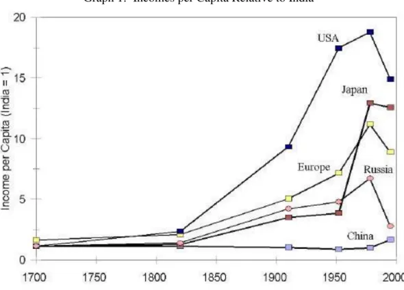
Although these former Atlantic slave economies eventually began to grow again, only the
US south has closed the gap with the richer regions. Even so it took nearly 100 years to do so. Most
of the world’s economies also have not closed the gap, as these regions are clearly among the richest (See Graph 1 in Appendix C). How then can we generalize the argument to the point where
it can become a growth theory valid for all economies?
The argument of the theory is that if world market prices and technology did not change at
abolition, those former slave economies which were unable to maintain the hierarchical managerial
structure with free workers would not reproduce the higher productivity of the plantations. The
formal microeconomic argument is now well understood. If the cost of supervision is lower than the
(welfare) loss to both of two complementary agents in a more lucrative, joint activity that is made
unviable due to one party (the principal) having to pay out more to the other (the agent) than the
value of the latter’s outside option in order to get him to perform in the joint activity at the correct level without supervision, then both can gain by a supervisory coordinating and monitoring scheme.
A rough measure of the static welfare loss after abolition is the fall in GDP.
The underlying economic rationale for these managerial structures, we suggest, is that for
hazard problems in the employer-employee transactions were less productive than the managerial
hierarchies. The historiography of the so-called, second industrial revolution abounds with studies
of the large-throughput, continuous process industries which needed them – steel, chemicals from coal, petroleum refining, electricity generation, the processing of vegetable oils etc. If it were not
for its labor and land intensive agricultural operations, cane sugar production and refining would fit
easily into this category. The relevant generalization then is that if an economy was unable to
implement with free workers, the management schemes of these large production units, whether in
agriculture or industry, it will not accompany the growth in incomes of the emerging leaders.
There were, of course, some economies which achieved high incomes by 1900 without
many such structures or even significant industrial activity. For example we can mention the
success of the family wheat farms of the US mid-west. These economized on managerial
supervision despite the introduction of machines which in turn required larger areas for each farm.
In more populous Western Europe, this transition would be less viable, at least for low value crops
like grains. The other rich, primary exporters of the period such as Australia and Argentina
demonstrate characteristics that seem to allow a similar explanation. And to take the opposite type
of exception, there were those economies which set up the more productive, hierarchical structures
in only one or two sectors while leaving the workers in the rest at near subsistence, the phenomenon
of dualism.
The common element in the success at growth, when it occurs, of either type of governance,
namely managerial structures or pulverized units, is technical progress. So the correct underlying
hypothesis is whether an economy can provide the incentives for the generation and implementation
of technological innovations, and not so much the type of production unit. However, if the activity
requires managers for economic viability and growth, then it is likely that a former slave economy
would be less able to sustain it for lack of consensus over the incentives. Various mechanisms for
third party interventions (labor legislation, trade unions and labor courts) may be required,
especially at start-up when the firm still has no reputation for fair treatment of its workers. If these
were missing or ineffective, it is likely that the economy will not introduce such innovations and
will stagnate even when it obtains workers from elsewhere whose opportunity costs are lower than
its former slaves.
As a tentative hypothesis we suggest that one legacy of slavery and abolition, which may
well be shared by other environments, is the inability to sustain large firms which use supervision as
a mechanism in their incentive schemes. Although there are many activities in a rich economy
which are done by small, family businesses which operate mainly in spot markets with marginal
bought, from the true engines. The other main type of production unit to generate innovations is the
public and quasi public enterprises like state companies and research universities. These can
replicate most of the mechanisms for supervised labor mobilized by the monopolies and oligopolies
of modern capitalism. The supervisors however would not be subject to the discipline of the capital
market, which implies that the incentives they offer to their supervised may well be different in
spite of the labor markets both institutions face.
This insight for growth theory comes from a comparison between the US north and south in
the late 19th century. By 1890, when the first federal law against cartels was passed (the Sherman
anti-trust act), large enterprises were being put together in several sectors in the US north – petroleum and sugar refining are two famous examples. Such institutions were absent from early
British capitalism which had served as the model for the neoclassical theory. We surmise that these
“big businesses”, the visible hand of monopoly power, were the crucial ingredient in the US overtaking the British level of income before 1914.
So a general growth theory for all economies may be the ability or otherwise to sustain
large enterprises which use supervision and other complex incentive schemes to allocate labor.
Curiously, this is not a world of Solow’s marginal-product incentives and perfectly competitive markets which leave no economic role for the firm. In those sectors where in the 20th century some have become one of the two major sources of the innovations which drive growth, failure to do so
can be fatal. The secret may not have been just markets. It may have been how to decide on which
markets to suppress, to make room for the incentives of firms.
REFERENCES (not all given in De Castro (2004) are cited in this extract)
Bairoch, Paul (1993), “Was there a large income differential before modern development”, in
Bairoch, Economics and world history: myths and paradoxes, Univ. of Chicago Press, Chapter 9.
Barzel, Yoram, (1977), “An economic analysis of slavery”, Journal of Law & Economics 20: 87-110.
Coatsworth, John H. (1993), “Notes on the comparative economic history of Latin
America and the United States” in Walter L. Bernecker and Hans Werne
r Tobler (eds),
Development and Underdevelopment in America: Contrasts of Economic Growth in North
and Latin America in Historical Perspective,
Berlin, 10-30.
Contador, C.R.
e
C.L. Haddad (1975), “Produto real, moeda e preços: A experiência
brasileira no período de 1861-
1970”,
Revista Brasileira de Estatística
36(143): 407-440.
David, Paul and other authors (1979), in American Economic Review, March.De Castro, Steve (2001) “Modern slave plantations to firms and labor markets: incentive
theory for a growth disaster”,
Seminar, Fundação Getúlio Vargas, Rio de Janeiro.
http://epge.fgv.br/files/1049.pdf
.
--- (2004), “Wrong incentives for growth in the transition from modern slavery to firms and
labor markets: Babylon before, Babylon after”, Social & Economic Studies 53(2):75-116 (journal distributed on-line by Proquest periodicals).
--- (2005), “A transição da escravidão moderna para mercados de trabalho e firmas: teoria
microeconômica para um desastre de crescimento na América”, Revista do Instituto Arqueológico, Histórico e Geográfico Pernambucano No. 61, July.
Domar, E. D. [1970], “The causes of slavery and serfdom: a hypothesis”, Journal of Economic history 30: 18-32.
Eisenberg, Peter L. (1974), The sugar industry in Pernambuco, 1840-1910: Modernization
without change, University of California Press.
Engerman, S.L. and K.L.Sokoloff [1997], “Factor endowments, institutions and differential paths of growth among New World economies: a view from economic historians of the United
States” in Stephen Haber (ed), How Latin America fell behind: Essays on the economic histories of Brazil and Mexico, 1800-1914, Stanford UP: 260-304.
Feenstra R. & G. Clark [2001], “Technology in the great divergence”, NBER WP#8596.
Fogel, R. W. and S. L. Engerman (1974), Time on the cross, Little, Brown.
Furtado, Celso (1963), The economic growth of Brazil, Univ. of California Press (original
1959).
Haddad, C.L. (1974),
The growth of real output in Brazil, 1900-1947
, PhD thesis,
University of Chicago.
Hall, Douglas (1978),
“The flight from the estates reconsidered: the British West Indies,1838-42”, J. of Caribbean History 10 – 11: 7-24.Hart, O. and J. Moore (1990), “Property rights and the nature of the firm”, J. of Political
Economy 98: 119-58.
Holmstrom, B.(1999), “The firm as a sub-economy”, J. of Law, Econ. & Org. 15(1): 74-102.
Holmstrom, B. and P.Milgrom (1994),“The firm as an incentive system”, Amer. Econ. Review
84: 972-991.
Irwin, James R. [1994], “Explaining the decline in southern per capita output after
Leff, N.
(1972), “A technique for estimating income trends
from currency data and an
application to nineteenth-
century Brazil”,
Review of Income and Wealth
18(4)
Dec.:335-368.
--- (1982), Underdevelopment and development in Brazil, Vol.1: Economic structure
and change, 1822-1947, George Allen & Unwin.
Lucas Jr, Robert E. (2002), Lectures on economic growth, Harvard UP.
Maddison, Angus(1995), Monitoring the world economy, 1820-1992, OECD.
Makowski, L. and J. M. Ostroy (1995), “Appropriation and efficiency: A revision of the first
theorem of welfare economics”, Amer. Econ. Review 85(4): 808-27
.
Martins, Roberto B. and Martins Filho, Amílcar, “Slavery in a non-export economy: a
reply”,Hispanic American Historical Review 64(1): 135-146.
Moohr, Michael(1972), “The economic impact of slave emancipation in British Guiana, 1832 –
52”, Econ. History Review (second series) 25: 588-607.
Pomeranz, Kenneth (2000), The great divergence: China, Europe and the making of the modern world economy, Princeton UP.
Ransom, Roger and Sutch, Richard (1975),
“The ‘lock
-
in’ mechanism and
overproduction of cotton in the post-bellum south
”
,
Agricultural History
49 (April):
405-425.
Rajan, R. and L. Zingales (1998), “Power in a theory of the firm”, Quarterly J. of Econ. 113(2): 387-432.
Reid Jr., Joseph D. (1973), “Sharecropping as an understandable market response: The post
-bellum south”, J. of Econ. History 33(1): 106-30.
Shapiro, C. and J. E. Stiglitz (1984),“Equilibrium unemployment as a worker disciplinary
device”, Amer. Econ. Review 74(3): 433-44.
Versiani, Flávio (1994), “Brazilian slavery: toward an economic analysis”, Revista Bras. de Economia 48 (4): 463-77:
Appendix A
( i) Proof of the envelope result (ii) in section 4.3. This analysis assumes that e e1, 2 0.
1. MAX I
pR e
1 e2
f e e
1, ;2
s.t.
e
1
e
2
0
or
g
e
1,
e
2;
0
Let the optimal solution be IS, 1S
,
2S
S S
S
e
e
pR
I
1
22. By the envelope theorem:
S S
S e e pR g f I 2 1
3. Find
, the Lagrange multiplier for this problem:
pRe1 e2 e1 e2 L
1 01 e R p e L 0 2 e L 0 2
1
e e
L
S S
S e e pR I 2
1 QED
(ii) Proof of result (i) in section 4.3 is similar.
(iii) Proof of
B p
p
A p
in section 4.6(a) We need to prove: if
Y
S
Y
F and
e
1S
e
2S
e
1F
e
2F
, then p < A(p)1.
Y
S
Y
F
pR
e
1S
e
2S
pR
e
1F
e
2F2. Add
e
2S
e
2F
e
1F
e
1S
to both sides and rearrange:
S F
S Fe
e
e
R
e
R
p
1
1
1
13. Multiply by –1 and rearrange gives the result (a) QED
(b) We need to prove: if IF > IS and
e
1S
e
2S
e
1F
e
2F
, then p > B(p)The proof is similar to result (a).
Appendix B
Proof that firms are never redundant in the Cobb-Douglas case:
R
e
1
e
1(see section4.4).
(i) Substitute
R
e
1
e
1in the envelope result from appendix A:
1 1 1 1 1 1 2 2 S F I p I p If
1 andp
1
then , 0 F S I
I at
1
To get IS IF
for 0
1, we must also have < 1.(ii) To get IF > IS, for 0<
1 we must have:1 1
1 1 1 1 1 1
p p
p p p p
After manipulation, this becomes:
1 1 1 p p p
which reduces to
1,
p
0, 0
1
. QEDAppendix C
GDP/head: Selected Countries, Americas, 19th century*
Moohr Eisner Moohr Eisner Atack & Passell Coatsworth Maddison
British
Guiana Jamaica
British
Guiana Jamaica US
South US
Midwest USA
Total USA Cuba Brazil Brazil USA UK
£const. 1912 1910
$
current
. $ const. 1985 $ const. 19901775 60
1800 807 904 738
1820 74 670 1287 1756
1830 92
1832 23.9 15.6 100 65
1840 74 65 109
1850 19.4 12.2 77 45 1394 1087 901
1860 103 89 128
1870 20.7 11.9 95 55 740 2457 3263
1880 791 205
1890 22.4 12.4 121 67
1900 1284 704 4096 4593
1910 24.0 13.7 117 67
1913 2004 3992 4854 1893 700 839 5307 5032
1920
1930 15.7 93 4664 8473