Emissions of terpenoids, benzenoids, and other biogenic gas-phase organic compounds from agricultural crops and their potential implications for air quality

www.atmos-chem-phys.net/14/5393/2014/ doi:10.5194/acp-14-5393-2014

© Author(s) 2014. CC Attribution 3.0 License.

Emissions of terpenoids, benzenoids, and other biogenic gas-phase

organic compounds from agricultural crops and their potential

implications for air quality

D. R. Gentner1,*, E. Ormeño2,3, S. Fares2,4, T. B. Ford5, R. Weber2, J.-H. Park2, J. Brioude6,7, W. M. Angevine6,7, J. F. Karlik8, and A. H. Goldstein1,2

1_{Department of Civil and Environmental Engineering, University of California, Berkeley, CA 94720, USA}

2_{Department of Environmental Science, Policy and Management, University of California, Berkeley, CA 94720, USA} 3_{Aix-Marseille Université – Institut méditerranéen de biodiversité et écologie IMBE CNRS UMR 7263, France}

4_{Consiglio per la Ricerca e la sperimentazione in Agricoltura (CRA)- Research Centre for the Soil-Plant System, Rome, Italy} 5_{Department of Chemistry University of California, Berkeley, CA 94720, USA}

6_{Cooperative Institute for Research in Environmental Sciences, University of Colorado, Boulder, CO 80309, USA} 7_{Chemical Sciences Division, Earth System Research Laboratory, National Oceanic and Atmospheric Administration,}

Boulder, CO 80305, USA

8_{University of California Cooperative Extension, Kern County, CA, USA}

*_{now at: Department of Chemical & Environmental Engineering, Yale University, New Haven, CT 06511, USA}

Correspondence to:D. R. Gentner (drew.gentner@yale.edu)

Received: 9 September 2013 – Published in Atmos. Chem. Phys. Discuss.: 1 November 2013 Revised: 28 March 2014 – Accepted: 11 April 2014 – Published: 3 June 2014

Abstract. Agriculture comprises a substantial, and increas-ing, fraction of land use in many regions of the world. Emis-sions from agricultural vegetation and other biogenic and anthropogenic sources react in the atmosphere to produce ozone and secondary organic aerosol, which comprises a sub-stantial fraction of particulate matter (PM2.5). Using data

from three measurement campaigns, we examine the mag-nitude and composition of reactive gas-phase organic car-bon emissions from agricultural crops and their potential to impact regional air quality relative to anthropogenic emis-sions from motor vehicles in California’s San Joaquin Valley, which is out of compliance with state and federal standards for tropospheric ozone PM2.5. Emission rates for a suite of

terpenoid compounds were measured in a greenhouse for 25 representative crops from California in 2008. Ambient mea-surements of terpenoids and other biogenic compounds in the volatile and intermediate-volatility organic compound ranges were made in the urban area of Bakersfield and over an or-ange orchard in a rural area of the San Joaquin Valley during two 2010 seasons: summer and spring flowering. We com-bined measurements from the orchard site with ozone

1 Introduction

Biogenic compounds are emitted from vegetation via sev-eral mechanisms and pathways. Emissions are typically a function of environmental parameters (e.g., light, tempera-ture) or specialized responses to communicate with, attract, or repel animals, insects, or other plants (Bouvier-Brown et al., 2009; Goldstein and Galbally, 2007). Biogenic emissions from plants are mostly in the gas phase and span from 1 to over 20 carbon atoms in size (Goldstein and Galbally, 2007). Examples include small compounds such as methanol and acetone, and a broad suite of isomers that are multiples of isoprene (C5H8). Prominent examples of these olefinic

com-pound classes include monoterpenes (C10H16) and

sesquiter-penes (C15H24). Their oxygenated counterparts contain 1–2

oxygen atoms and are included in the definition of monoter-penoids and sesquitermonoter-penoids. Plant species can emit a vari-ety of these isomers with one or more double bonds and can include cyclic or bicyclic rings, but a certain suite of com-pounds has been observed more frequently (Bouvier-Brown et al., 2009; Goldstein and Galbally, 2007). Commonly re-ported monoterpenes include 1-limonene, α-pinene, and

13-carene; common sesquiterpenes, which are more diffi-cult to measure, include β-caryophyllene and α-humulene (Bouvier-Brown et al., 2009; Helmig et al., 2006; Ormeno et al., 2007, 2010). Many terpenoids have specific functions and are responsible for the fragrances and flavors associated with various plants (Bouvier-Brown et al., 2009; Lewis et al., 2007; Afsharypuor and Jamali, 2006; Bendimerad et al., 2007; Bernhardt et al., 2003; Azuma et al., 2001; Omura et al., 1999; Kotze et al., 2010). Some studies have also shown plant leaves or flowers to contain other compounds with aro-matic rings (i.e., benzenoids) and nitrogen- or sulfur-based functional groups (Lewis et al., 2007; Afsharypuor and Ja-mali, 2006; Bendimerad et al., 2007; Bernhardt et al., 2003; Azuma et al., 2001; Omura et al., 1999; Kotze et al., 2010; Ormeno et al., 2010).

Much work has been done to understand emissions of bio-genic gas-phase organic carbon since most of the compounds are highly reactive and can produce ozone (O3) and

sec-ondary organic aerosol (SOA) as a product of their chemistry with atmospheric oxidants (Carter, 2007; Ng et al., 2006). Studies on gas-phase organics in the past decade have ob-served evidence for unknown biogenic emissions that could not be chemically resolved (Di Carlo et al., 2004; Holtzinger et al., 2005). Subsequent research has expanded the range of measurements (Bouvier-Brown et al., 2009; Helmig et al., 2006; Ormeno et al., 2007, 2010), and further characteri-zation remains necessary. Additionally, understanding emis-sions from vegetation is important because of the complex interplay of anthropogenic emissions and biogenic emissions from both natural vegetation and agricultural crops, in Cal-ifornia and globally (Spracklen et al., 2011; Shilling et al., 2013). Agricultural plantings make up a major fraction of land cover in some regions such as California’s San Joaquin

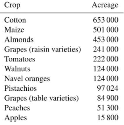
Table 1.Planted areas for permanent crops with largest land cover in the San Joaquin Valley.

Crop Acreage

Cotton 653 000

Maize 501 000

Almonds 453 000

Grapes (raisin varieties) 241 000

Tomatoes 222 000

Walnuts 124 000

Navel oranges 124 000

Pistachios 97 024

Grapes (table varieties) 84 900

Peaches 51 300

Apples 15 800

Data from 2002 crop reports, respective county agriculture commissioners’ offices.

Valley (Fig. S1), which is an extreme non-attainment area for ozone and a non-attainment area for PM2.5(US EPA). A

summary of prominent agricultural crops in the San Joaquin Valley is shown in Table 1. Historically, there has been some research on emissions from agricultural crops in California (Arey et al., 1991a, b, c, d; Winer et al., 1989; Winer et al., 1992; Karlik et al., 2002). However, biogenic emissions from many of these crops and other agricultural plants require fur-ther characterization with new advances in instrumentation and contemporary scientific knowledge and concerns. Also, total emissions have previously been thought to be minor rel-ative to natural vegetation (Lamb et al, 1987), and further measurements of terpenoid emissions are necessary to build upon previous work. Models on regional scales, and larger, need this information on emission factors from individual plant species to improve parameterizations; these include the MEGAN (Model of Emissions of Gases and Aerosols from Nature) model (Sakulyanontvittaya et al., 2008; Guenther et al., 2012) and the BEIGIS (Biogenic Emission Inventory Ge-ographic Information System) model developed by the Cali-fornia Air Resources Board (2003).

2 Materials and methods

This paper uses measurements from three campaigns: a sur-vey using plant and branch enclosures in a greenhouse, a multi-season campaign in an orange orchard, and an urban site in Bakersfield, CA. The principle gas-phase organic car-bon measurements in this work were made using a custom gas chromatograph with a mass spectrometer and a flame ionization detector (GC/MS-FID). A broad suite of several hundred compounds was quantified with hourly time reso-lution. Extensive detail on the design and operation of the instrument can be found in Gentner et al. (2012).

To examine emissions from agricultural vegetation, 25 dif-ferent crops were studied in the partially controlled environ-ment of the Oxford Tract greenhouse at UC Berkeley during the summer of 2008 (all experiment design details available in Fares et al., 2011). The crops included a mixture of woody trees and shrubs, as well as herbaceous plants that are promi-nent in California (Table S1), with emissions from 2 to 8 in-dividual plants measured for each species. Plants were all potted, fertilized weekly, and watered daily to provide good growing conditions and avoid water stress. Plants were ex-posed to natural sunlight and the greenhouse humidity was maintained at 40–60 %. Depending on plant size, branches or whole plants were enclosed in custom Teflon chambers outfitted with temperature and light monitors, and supplied with purified “zero” air (Aadco model 737) enriched with carbon dioxide. Measurements were performed for several days at a time, with additional replicates of each species. To avoid any biases caused by plant damage during enclosure, plants were given time to equilibrate before measurements were used to assess emission rates and chemical speciation. In addition to chemically speciated measurements of VOCs and IVOCs via gas chromatography–mass spectrometry, sev-eral other instruments were used to measure ozone, carbon dioxide, and water vapor. Measurements of isoprene and monoterpenes reported from greenhouse enclosure measure-ments were made in conjunction with a high-time-resolution proton transfer reaction mass spectrometer (PTR-MS) (Fares et al., 2011).

Following the greenhouse study wherein orange trees were among the largest emitters, a yearlong measurement site was set up in a Valencia orange orchard in the San Joaquin Valley (36.3566◦N, 119.0923◦W). The site was located in Lind-cove, which is east of the city of Visalia near the foothills of the Sierra Nevada. The local area around the site had a large planted area of various citrus trees and some other crops. In addition to biogenic emissions from nearby agriculture, the site was influenced by natural vegetation in the surrounding mountains and anthropogenic sources in the San Joaquin Val-ley. A detailed description of the site can be found in Fares et al. (2012b). We took two sets of chemically speciated or-ganic carbon measurements at this site during two different seasons: in April–May 2010 during citrus flowering and sum-mer 2010 (each 10 or more days). Measurements were made

at the top of the canopy (4 m), and the site had a similar suite of supporting measurements as the greenhouse study. Year-long measurements of ozone fluxes over the orange orchard are used in this work; these methods have been described elsewhere (Fares et al., 2012b).

Ambient in situ measurements were made in Bakersfield, CA, at the CalNex (California Research at the Nexus of Air Quality and Climate Change) supersite (35.3463◦N, 118.9654◦W) located in southeastern Bakersfield in the southern San Joaquin Valley. Measurement of gas-phase or-ganics took place during the period of 18 May–30 June 2010, sampled from the top of an 18 m tower. To reduce losses of highly reactive compounds in the sampling system, ozone was removed at the inlet using sodium thiosulfate-treated fil-ters at both ambient measurement sites (discussed in Gentner et al., 2012).

We recently developed a method in Gentner et al. (2014) that calculates the spatial distribution of emissions in a region based on fixed-location measurements and coinci-dent footprints for each hourly sample determined using the FLEXPART-WRF Lagrangian model for meteorological modeling (Brioude et al., 2012). Extensive details on the methodology can be found in Gentner et al. (2014). In this work, we use it to examine the transport of biogenic VOCs to the urban site in the southern San Joaquin Valley.

Basal emission factors (BEFs) are the standardized emis-sion factors for biogenic compounds from vegetation, and are adjusted based on the environmental parameters consid-ered. BEFs were calculated for each compound class for each plant species studied in the greenhouse by taking the aver-age of the data points with temperature = 30±2◦_{C, and}

pho-tosynthetically active radiation (PAR)>800 µmol m−2_s−1_.

These emission rates, or fluxes, are reported in carbon mass per mass dry leaf matter per time (e.g., ngC gDM−1h−1). If insufficient data existed at these basal conditions, data were logarithmically extrapolated from lower temperature data to determine BEFs (see Fares et al. (2011) for details).

of determination (r2) are reported to describe how accurately each method models the emissions from each plant and com-pound class in this study.

At the Lindcove and Bakersfield sites, comparisons of bio-genic to anthropobio-genic burdens of gas-phase organic car-bon were done using chemical mass balance source receptor modeling methods (Gentner et al., 2012) to model anthro-pogenic emissions from motor vehicles. Total emissions of anthropogenic hydrocarbons in the San Joaquin Valley from motor vehicles are determined using the emission factors de-rived in Gentner et al. (2012) and fuel use data for the seven counties in the air basin (California Dept. Transportation, 2008). Our estimates of biogenic emissions for the region were compared to the California Air Resources Board emis-sion inventory (2010). The ozone formation potential of these emissions are compared as maximum incremental reactivity (MIR) values for each compound (or compound class) cal-culated by Carter (2007) using the SAPRC (Statewide Air Pollution Research Center) chemical mechanism. Existing information on yields of secondary organic aerosol from at-mospheric oxidation are compiled from the literature (Gen-tner et al., 2012; Saathoff et al., 2009; Kim et al., 2012; Ng et al., 2006). Where available, literature values are presented for reaction constants of atmospheric oxidants with the bio-genic compounds measured in this study (Atkinson and Arey, 2003a, b). Otherwise, for newly measured compounds, the-oretical values are estimated using the US EPA’s EPI Suite program (2000).

3 Results and discussion

3.1 Greenhouse measurements of individual plant species

There were numerous terpenoid compounds quantified in emissions from crops with considerable diversity of emis-sions between plant species. Emission parameters and de-tailed chemical speciation for monoterpenes, oxygenated monoterpenes, and sesquiterpenes measured from the differ-ent crops in the greenhouse study are shown in Tables 2 and S2–S5. With the exception of two orange trees, all plants were in a non-flowering state. Monoterpene concentrations were measured as individual species via gas chromatogra-phy and as total monoterpenes with the PTR-MS, and agreed to within 20 % (Fares et al., 2011). In addition to the well-known monoterpenes1-limonene andα-pinene, there were similar magnitude emission factors forβ-myrcene, sabinene, and both isomers of β-ocimene. Oxygenated monoterpene emissions were dominated by linalool and perillene, a little-studied furanoid. We observed only two sesquiterpenes, α -humulene andβ-caryophyllene, from the crops studied. Con-sistent with previous work,β-caryophyllene dominated the two, but it is likely that there were other sesquiterpenes out-side of the observable range, at concentrations below the

limit of detection, or lost in the sampling system prior to detection. A broader suite of sesquiterpenes was measured using a cartridge method and emission factors are reported by Ormeno et al. (2010).

Calculated BEFs and beta values for total monoterpenes, oxygenated monoterpenes, and sesquiterpenes are summa-rized in Table 2 with relevant statistical metrics. Data on the chemical speciation of emissions and the performance of the temperature-only and light+temperature modeling methods are shown in Tables S2–S5. Compared to other natural veg-etation (e.g., oak trees, poplar) agricultural crops have low isoprene emission factors. This work focuses on the larger emissions of terpenoids, but a summary of observed isoprene fluxes can be found in Tables S6–S7 along with emission fac-tors for methanol, acetaldehyde, and acetone. While it is con-ventionally helpful to group plants together for the purposes of modeling based on either emissions strength or crop type, we have refrained from doing so in this work. There is a con-siderable amount of uncertainty in the individual emission factors and the relative strength of emissions varies for each plant species depending on chemical class. Such a grouping would be subject to the limitations of this study and, in some cases, regional assumptions.

3.1.1 Monoterpenes

Total emissions of monoterpenes were lowest (<100 ngC gDM−1h−1) from almond, grape, olive, pistachio, plum, and pomegranate (Table 2). For almond and cherry, the monoterpene BEF agreed with previous research (Winer et al., 1992). Emissions from grapes were very low (11 and 91 ngC gDM−1_h−1_{), and Winer et al. (1992) did}

not detect any emissions. The monoterpene BEF for peach, 1211 ngC gDM−1h−1, was significantly higher than other plants in thePrunusgenus (i.e., almond, plum) measured in this study.

Correlations between measured and modeled monoter-pene emissions for both the temperature-only and the light + temperature modeling methods were significant for almond and olive (Table S2). Some plant species, such as the above-mentioned, are known to have storage structures on their leaves where terpenes are typically stored (Vieira et al., 2001). The existence of these “pools” of biogenic com-pounds is relevant since harvesting or pruning may cause emissions if leaves are damaged during agricultural opera-tions.

Table 2.Basal emission factors (ngC gDM−1h−1) and beta values for monoterpenes, oxygenated monoterpenes, and sesquiterpenes from enclosure studies (Nis the sample size andrthe correlation coefficient).

Monoterpenes Oxygenated monoterpenes Sesquiterpenes

Crop BEF±SD (N) Beta (r)(N) BEF±SD (N) Beta (r)(N) BEF±SD (N) Beta (r)(N)

Alfalfa 270±160 (2) 0.10 (0.84)(11) N.D. N.D.

Almond 68±51 (23)[24] _{0.065 (0.23)(157)}∗ _{150±28 (6)}[24] _{0.16 (0.90)(32) 10 000±3300 (6)}[24] _{0.45 (0.92)(31)} Carrot (RL) 78±45 (15)[25] N.B. 22±12 (3)[25] 0.099 (0.51)(11) N.D.

Carrot (BN) 48±36 (43)[27] 0.063 (0.29)(166)∗ 56±36 (3)[27] N.B.

Cherry 84±59 (26)[26] _{0.067 (0.34)(121)}∗ _{670±250 (16)}[26] _{0.30 (0.94)(40) N.D.}

Corn N.D. N.D. N.D.

Cotton Pima 47±21 (10)[27] _{0.027 (0.25)(31)}∗ _{2700±3100 (5) 0.13 (0.35)(26) N.D.}

Cotton upland 41±16 (4) 0.12 (0.74)(16) 81±83 (4) 0.18 (0.26)(7) N.D.

Table grape 11±4.9 (2)[28] N.B. 26±13 (5) 0.029 (0.27)(23) 45±15 (5) 0.095 (0.69)(13)

Wine grape 91±50 (13)[27] _{0.17 (0.67)(20) 44±10 (3)}[25] _{N.B. 52±22 (8)}[27] _N.B.

Liquidambar 350±260 (31)[26] 0.098 (0.35)(174)∗ 47±4.8 (2)[26] 0.19 (0.94)(4) N.D.

Miscanthus 140±89 (17)[27] 0.044 (0.20)(63)∗ 48±19 (6)[28] 0.16 (0.80)(11) 180±31 (6)[28] 0.076 (0.76)(11) Olive 60±32 (8)[26] _{0.15 (0.68)(28) 7.5±0.91 (2)}[26] _{0.066 (0.51)(4) N.D.}

Onion 350±110 (3)[28] N.B. N.D. N.D.

Peach 1200±270 (2)[24] _{0.23 (0.97)(10) 240±55 (2)}[24] _{0.23 (0.97)(10) N.D.} Pistachio 40±22 (47)[28] 0.098 (0.47)(207)∗ 39±55 (15)[26] 0.15 (0.36)(22)∗ N.D. Plum 37±20 (5)[26] 0.010 (0.04)(26)∗ 30±11 (4)[28] 0.14 (0.68)(6) N.D.

Pomegranate 32±26 (4)[25] _{N.B. 26±9.8 (4)}[27] _{0.14 (0.78)(5) 61±8.6 (5)}[27] _{0.024 (0.23)(9)*}

Potato 150±9.8 (3)[24] 0.064 (0.47)(16)∗ 22±9.3 (3)[27] N.B. 40±13 (3) N.B.

Tomato 740±260 (7)[27] 0.11 (0.31)(68)∗ N.D. 59±15 (3)[27] N.B.

Orange P.N. (no flowers) 2500±3400 (116)[26] _{0.14 (0.35)(522)}∗ _{1300±1900 (33)}[26] _{N.B. 1500±970 (20)}[25] _{0.25 (0.74)(58)} Orange P.N. (flowers) 7800±4300 (36)[26] 0.15 (0.71)(151) 4600±1300 (11)[24] 0.072 (0.38)(36)∗ 3200±780 (11)[24] 0.28 (0.92)(36) Mandarin W. Murcott 63±25 (20)[28] 0.080 (0.47)(99)∗ 150±190 (8)[29] 0.23 (0.79)(20) N.D.

Mandarin clementine 26±18 (22)[26] _{0.064 (0.27)(141)}∗ _{N.D. N.D.}

Lemon Eureka 22±22 (24)[25] 0.036 (0.15)(166)∗ N.M. N.M.

Notes: N.M. stands for no measurements; N.D., below detection limit; N.A., no basal condition met; and N.B., beta value analysis inaccurate.

When the basal emission factor (BEF) was determined at a lower temperature and adjusted, the temperature it was determined at is indicated after the BEF as[C]_{, the value was adjusted using the calculated beta} unless the correlation coefficient for beta was below 0.5, then a default beta of 0.1 was used and the beta column is marked with∗_.

The BEF sample size is the number of measurement samples used to determine the BEF, while the sample size in the beta column refers to the number of measurement samples where the compound classes were observed and used to calculate the beta value.

Data on citrus species measured in the same greenhouse campaign are reproduced from Fares et al. (2011) for comparison to the other crops and assessment of implications on air quality. Chemical speciation of emissions can be found in Tables S2–S5.

suggesting that higher emissions should be expected during harvesting.

Parent navel orange (P. N. orange) had a high monoterpene emission factor with a beta coefficient of 0.14 without flow-ers (temperature only algorithm), which is consistent with previous published work on oranges (Ciccioli et al., 1999). Emissions of total monoterpenes from other citrus species in this study were very low: 22, 26, and 63 ngC gDM−1h−1for Eureka lemon, clementine mandarin, and W. Murcott man-darin, respectively. Monoterpene emissions from P. N. or-ange were predominantlyβ-myrcene andβ-trans-ocimene, and mandarins emitted mainlyβ-cis- and β-trans-ocimene. Previous work has shown much higher emission for Lisbon lemons (Winer et al., 1992), which suggests potential vari-ability in emissions owing to phenological factors.

Our emission measurements of pistachio are considerably lower than previous work classifying pistachio as a large monoterpene emitter; our BEF is more than 2 orders of mag-nitude lower than in Winer et al. (1992). Since pistachio acreage is very large in California, further studies on this crop are warranted as fundamental questions remain about pistachio’s BEF. It is possible that although the same variety was used in both studies, specific phenotypic traits of the in-dividuals selected could cause such differences. It is the case

here with pistachio, as with many other crops surveyed in our study, that several replicates of a few individuals for a crop variety were likely inadequate to capture the variability in biogenic emissions within individuals of the same species, between different crops, and during different periods of an individual’s life or annual cycle. The results of this portion of the study are also subject to the limitations of the green-house environment, compared to the field; plants were potted and were exposed to lower than typical light and temperature conditions. Thus, it is important to note that the results pre-sented from the greenhouse study comprise a survey of emis-sions from a broad suite of crops, and more extensive mea-surements are critical to effectively characterize emissions from a particular crop species. Future users of these individ-ual crop data should be cautious of the variability between individuals of the same species and their seasonal cycles.

3.1.2 Oxygenated monoterpenes

(BEF = 4600 ngC gDM−1_h−1_{), followed by Pima cotton}

and non-flowering orange (2700 and 1300 ngC gDM−1_h−1_,

respectively). Lower emissions were observed from cherry, peach, almond, and W. Murcott mandarin, with very low emissions from the other crops (Table 2). Modeled and measured emissions of oxygenated monoterpenes from non-flowering orange trees were not well correlated. The occurrence of perillene may suggest that neither of the modeling methods represents emissions of this furanoid. For flowering oranges, the temperature only method best describes the emission of oxygenated monoterpenes, mainly linalool, confirming the temperature dependency of linalool emissions reported previously (Ciccioli et al., 1999).

3.1.3 Sesquiterpenes

Almond was the highest sesquiterpene emitter of the crops studied according to the calculated BEF (10000 ngC gDM−1h−1), while the magnitude of the monoterpene and oxygenated monoterpene emissions was very low. This sesquiterpene BEF was anomalous, so we report it with low confidence. The calculated beta of 0.45 is very high, and all the measurements for almond were below 25◦C. Using a beta of 0.1, the BEF would be 1200 (a factor of 10 lower, but still a significant emission). Sesquiterpene emissions were very low or not detected for other non-citrus woody crops. Sesquiterpene emissions from tomato were 59 ngC gDM−1h−1, slightly lower than the range reported in previous work for different varietals (Winer et al., 1992). After almond trees, P. N. orange trees had the highest sesquiterpene emission rates, with the flowering specimen being twice that of the non-flowering trees.

3.2 Emissions from flowering citrus trees

Many trees and herbaceous plants produce flowers once or more every year. In the greenhouse enclosure studies, flow-ering increased monoterpene emissions from orange trees by a factor of 3 with only a few flowers (a lower density than observations at the field site). The presence of flowers has been shown previously to dramatically influence the magni-tude and composition of emissions from orange trees (Cicci-oli et al., 1999; Hansen et al., 2003; Arey et al., 1991a). In the greenhouse studyβ-myrcene andβ-trans-ocimene were the dominant monoterpenes emitted from orange trees (Ta-ble S3).β-cis-ocimene was also observed from the flowering plants. Emissions of the oxygenated monoterpene linalool increased by a factor of∼3.5 from the flowering plant.β -caryophyllene emissions also increased by a factor of 2 for the flowering orange tree. Increased emissions from the flow-ering orange tree were observed for all compounds measured (Fares et al., 2011), but the otherCitrusspecies had no flow-ering individuals for comparison.

During the spring field measurement campaign at the or-ange orchard, a broad array of biogenic gas-phase organic

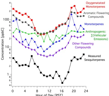
Figure 1.Average diurnal patterns of different compound classes shown on a logarithmic scale during flowering at the Lindcove site. Anthropogenic emissions from motor vehicles are shown for com-parison. Floral emissions of oxygenated monoterpenes and aromat-ics dominate total biogenic emissions. Measured sesquiterpenes are lower than total sesquiterpenes as not all sesquiterpenes could be observed/quantified.

compounds was measured in ambient air (Table 3). Flower-ing occurrFlower-ing at the field site, and in the local area, had a major impact on the distribution of biogenic compounds in ambient air. There was a dramatic increase in both the mag-nitude and diversity of chemical species emitted during the flowering process. Due to strong nocturnal inversions, many were measured at ppb-level concentrations at night owing to their buildup in the shallow boundary layer where ozone had been scavenged to concentrations below 10 ppb. Perhaps of more interest is that daytime concentrations averaged above 10 ppt for most compounds, when their emissions are most relevant to photochemistry. Additionally, several of the most prominent compounds had daytime concentrations that regu-larly exceeded 1 ppb (Table 3).

Table 3.Interquartile ranges [pptv] for measured biogenic compounds in spring and summer.

Spring (flowering) Summer

Day Night Day Night

Compound (10:00–17:00) (20:00–06:00) (10:00–17:00) (20:00–06:00)

isoprene 24.8–67.4 55.5–375.8 61.3–197.8 107.4–852.8

α-thujene 3.8–13.7 16.4–122.0 2.5–3.7 4.6–19.1

α-pinene 6.9–13.0 12.6–90.8 3.2–6.8 5.4–20.7

camphene 4.4–6.8 6.2–40.2 3.7–7.7 7.0–26.5

sabinene 23.6–67.6 62.7–977.5 11.5–23.2 15.7–33.7

β-myrcene 324.1–1143.2 407.9–2285.4 4.4–9.3 8.4–49.8

β-pinene BDL–17.7 12.8–52.3

α-phellandrene 1.3–3.1 2.1–5.1 2.3–6.7 7.0–35.1

cis-3-hexenyl acetate 165.3–353.7 213.3–790.2

13-carene 23.0–51.1 37.0–162.0 3.2–5.2 5.2–38.5

Benzaldehyde 69.5–276.0 78.6–434.3

α-terpinene 5.3–12.0 12.0–102.1

cis-β-ocimene 23.9–65.9 39.5–162.5 trans-β-ocimene 134.8–380.3 197.6–1267.1

1-limonene 183.6–365.0 275.2–2250.5 158.9–271.9 204.1–1606.0

p-cymene 17.8–41.1 26.0–238.6 7.8–16.6 16.4–176.5

γ-valeroactone 6.2–11.3 11.2–103.3

γ-terpinene 16.4–32.4 30.6–247.6 1.6–7.5 4.1–15.5

terpinolene 6.7–15.6 14.2–85.8 1.7–2.7 6.8–22.2

trans-linalool oxide 1.7–5.1 3.3–18.0 cis-linalool oxide 9.2–14.9 11.6–50.6 benzeneacetaldehyde 57.1–242.4 86.8–455.7

linalool 1657.3–6037.5 2436.4–18 342.1

lavender lactone 122.5–278.6 216.3–1033.1

sabina ketone 16.8–111.9 58.8–255.1

2-amino-benzaldehyde 174.0–443.1 189.2–806.2

indole 984.6–2707.4 1408.4–3696.6

methyl anthranilate 906.6-2742.4 1151.8-6856.5 benzeneethanol 188.2–420.4 215.8–966.7 benzyl nitrile 836.6–1780.8 971.7–3212.2 methyl benzoate 14.9–32.8 19.8–57.6 β-caryophyllene 9.7–19.6 7.0–18.4

aromadendrene 7.2–25.0 10.2–31.9

trans-β-farnesene 3.1–21.5 6.9–41.7

valencene BDL–17.1 13.3–59.2

trans-Nerolidol 22.7–150.9 64.0–301.1

n-pentadecane 12.6–29.5 14.6–35.8

n-hexadecane 8.1–37.3 5.4–34.9

n-heptadecane 36.6–83.7 38.7–101.4

8-heptadecene 1.2–7.1 2.0–52.0

1-heptadecene 79.0–204.3 105.5–285.5

hexanal 35.8–162.7 81.0–337.8

octanal 11.6–25.3 17.3–73.9

nonanal 55.0–120.4 68.6–184.2

decanal 6.9–21.1 11.3–40.1

Notes: entries left blank indicate that compound was not observed during the summer campaign (sesquiterpenes could not be measured during the summer due to chromatographic and detector difficulties).

Table 4.Novel compounds from measurements of ambient air during flowering.

Name(s) Structure kOH [cm

3

s-1 molecules-1 *1011]

Lifetime to OH oxidation [min]

Indole 15.4 20

Methyl Anthranilate (benzoic

acid, 2-amino-, methyl ester) 3.48 89

Benzeneacetaldehyde

(phenyl acetaldehyde) 2.63 117

Benzeneethanol

(phenylethyl alcohol) 0.957 323

Benzyl Nitrile

(benzneacetonitrile) 0.962 321

Lavender Lactone (γ-lactone, dihydro-5-methyl-5-vinyl-2(3H)-furanone)

2.76 112

Methyl Benzoate

(Methyl Benzenecarboxylate, Niobe Oil)

0.0844 3660

Sabina Ketone (5-isopropylbicyclo [3.1.0]hexan-2-one)

0.626 493

2-amino-benzaldehyde 5.23 59

Notes:

Chemical Structures from NIST Chemistry WebBook http://webbook.nist.gov/chemistry/ [OH] = 0.25 pptv

not been previously reported in other studies of ambient air. These compounds were initially identified through high-quality matches to mass spectra libraries and Kovat’s in-dices for appropriate retention times, and then later con-firmed with authentic standards after the campaign. Table 4 summarizes their chemical structures and reactivity. Many of the compounds we observed during flowering have been attributed to floral scents or essential oils from flowers in various botany and ecology studies, which include a vari-ety of compounds with aromatic rings, as well as nitrogen, sulfur, and/or oxygen-containing functional groups (Lewis et al., 2007; Afsharypuor and Jamali, 2006; Bendimerad et al.,

2007; Bernhardt et al., 2003; Azuma et al., 2001; Omura et al., 1999; Kotze et al., 2010).

Given the novelty of the measurements for these com-pounds, no previous work validates the efficacy of mea-surement methods or interactions with ozone removal traps at the inlet. While additional measurement uncertainty is warranted, we are confident in the methods used for these compounds as we were able to accurately measure other compounds in their volatility range (C11−15) and greater

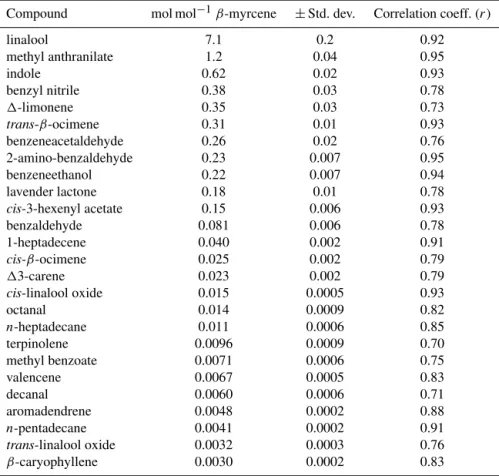
Table 5.Compounds well-correlated with flowering emissions (represented byβ-myrcene).

Compound mol mol−1β-myrcene ±Std. dev. Correlation coeff. (r)

linalool 7.1 0.2 0.92

methyl anthranilate 1.2 0.04 0.95

indole 0.62 0.02 0.93

benzyl nitrile 0.38 0.03 0.78

1-limonene 0.35 0.03 0.73

trans-β-ocimene 0.31 0.01 0.93

benzeneacetaldehyde 0.26 0.02 0.76

2-amino-benzaldehyde 0.23 0.007 0.95

benzeneethanol 0.22 0.007 0.94

lavender lactone 0.18 0.01 0.78

cis-3-hexenyl acetate 0.15 0.006 0.93

benzaldehyde 0.081 0.006 0.78

1-heptadecene 0.040 0.002 0.91

cis-β-ocimene 0.025 0.002 0.79

13-carene 0.023 0.002 0.79

cis-linalool oxide 0.015 0.0005 0.93

octanal 0.014 0.0009 0.82

n-heptadecane 0.011 0.0006 0.85

terpinolene 0.0096 0.0009 0.70

methyl benzoate 0.0071 0.0006 0.75

valencene 0.0067 0.0005 0.83

decanal 0.0060 0.0006 0.71

aromadendrene 0.0048 0.0002 0.88

n-pentadecane 0.0041 0.0002 0.91

trans-linalool oxide 0.0032 0.0003 0.76

β-caryophyllene 0.0030 0.0002 0.83

functionalized than the chemical species reported here. Nev-ertheless, the measurements we report are potentially lower limits in the event of chemical or physical losses in our sam-pling/measurement system.

There were several previously unidentified peaks ob-served during measurements of the flowering P. N. orange in the greenhouse studies that have very good retention time matches to these flowering compounds measured at this site, including indole, methyl anthranilate, benzeneethanol, ben-zyl nitrile, 2-aminobenzaldehyde, and possibly sabina ketone (Fig. S2). In the greenhouse measurements, these compounds were observed only from the flowering specimen, support-ing the conclusion that flowersupport-ing is the source. At the field site, daytime concentrations of methyl anthranilate, indole, and benzyl nitrile were over 1 ppb, similar or greater than the dominant monoterpeneβ-myrcene. Lavender lactone, benze-neethanol, 2-amino-benzaldehyde, and benzeneacetaldehyde had significant median daytime concentrations at, or above, 100 ppt. Sabina ketone and methyl benzoate had lower con-centrations similar to the linalool oxide isomers, but still ap-peared to be emitted in significant amounts. cis-3-Hexenyl acetate, a well-known plant-wounding compound (Fall et al., 1999), had considerable nighttime concentrations ranging 200–800 ppt despite no harvest or pruning activity, and corre-lated well with other flowering compounds, suggesting that it

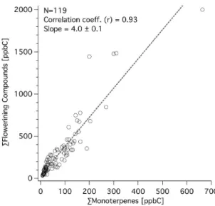
is also released as part of the flowering process. In addition to these compounds, we also observed several high-molecular-weight straight alkanes and alkenes associated with flower-ing (e.g.,n-heptadecane, 1-heptadecene), which have been reported in other floral and essential oil analyses (Lewis et al., 2007; Afsharypuor and Jamali, 2006; Bendimerad et al., 2007; Bernhardt et al., 2003; Kotze et al., 2010; Winer et al., 1992). Additionally, emissions of benzyl alcohol and ben-zaldehyde were recently observed in a flowering tree enclo-sure study (Baghi et al., 2012). At our field site, the diur-nal patterns of the flowering-related compounds were similar to that of monoterpenes, but were more prevalent (Figs. 1– 2). A regression of the flowering-related compounds to the sum of monoterpenes yielded a ratio of 4.0 (on a carbon mass basis), with the sum of monoterpenes also including compounds that were related to flowering (i.e.,β-myrcene, sabinene, and bothβ-ocimenes).

Figure 2. Comparison of total observed flowering compounds to the sum of monoterpenes during the spring at the Lindcove site. Concentrations were well correlated with a slope of 4.0, but can be expected to vary somewhat with the density of blossoms over the whole period of flowering. In addition to the flowering countdowns, large increases in monoterpenes concentrations were observed.

not necessarily imply lower emissions, but could also be a re-sult of sesquiterpene compounds reacting at more rapid rates in the atmosphere than other terpenoid compounds. Sam-pling methodology can sometimes be responsible for under-estimates of ambient concentrations, but the sampling and measurement techniques used in this study are suitable for sesquiterpene measurements (Bouvier-Brown et al., 2009; Pollmann et al., 2005). It is very likely that only a fraction of the emitted sesquiterpenes were measured due to their short atmospheric lifetimes, reacting with both OH and ozone.

We were only able to detect and identify a few sesquiter-penes. However, previous work (Ormeno et al., 2010) has shown that a wide array of sesquiterpenes are emitted from agricultural crops (flowering and non-flowering) and that emissions of sesquiterpenes should be roughly equivalent to those of monoterpenes. In the spring, measured sesquiter-penes were on average 5 % of monotersesquiter-penes by carbon mass, but flowering is an episodic event and is not representative of an annual average. Previous work with the MEGAN model estimates sesquiterpene emission to be 9–16 % of monoter-penes, but sesquiterpene data for input into the MEGAN model is limited (Sakulyanontvittaya et al., 2008). Figure 3 shows the relative amounts of sesquiterpenes to monoter-penes. It is evident that there is a dynamic range of observed ratios that varies over the course of the day and it is quite possible that additional, unaccounted for sesquiterpenes will increase the ratio.

The concentrations of sesquiterpenes during flowering were higher than previous work done in a ponderosa pine for-est, where concentrations of individual sesquiterpenes were on the order of 10 ppt (Bouvier-Brown et al., 2009), but

Table 6.Source profile (±Std. Dev.) for flowering emissions (non-monoterpene) from citrus trees.

Compound % mass

linalool 70.4±2.8 %

methyl anthranilate 12.1±0.5 %

indole 4.65±0.19 %

benzyl nitrile 2.86±0.21 % benzeneacetaldehyde 2.02±0.16 % 2-amino-benzaldehyde 1.79±0.07 % benzeneethanol 1.75±0.07 % lavender lactone 1.48±0.12 % cis-3-hexenyl acetate 1.38±0.06 % 1-heptadecene 0.61±0.03 % benzaldehyde 0.55±0.04 % n-heptadecane 0.16±0.01 % cis-linalool oxide 0.16±0.01 % methyl benzoate 0.06±0.01 % trans-linalool oxide 0.03±0.003 %

Note: the monoterpenesβ-myrcene andtrans-β-ocimene are also observed in large concentrations during flowering and can be expected as part of the source profile (relative ratios can be calculated from Table 5).

there are very few published ambient air measurements of sesquiterpenes with which to compare our observations. Our summertime measurements did not have the capacity to mea-sure sesquiterpenes due to chromatographic and detector dif-ficulties.

3.3 Seasonal differences in biogenic emissions

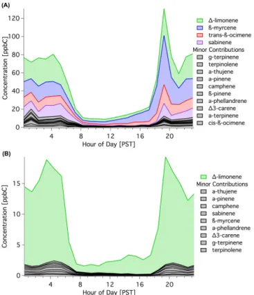
While there were considerable year-round concentrations of monoterpenes at the site, there was a strong increase in bio-genic emissions during the flowering period. A compari-son indicates that the daytime sum of monoterpenes dur-ing sprdur-ing flowerdur-ing was 6±1 times those in summer non-flowering conditions (Figs. 4–5)(10–16 PST prior to large changes in friction velocity in the late afternoon (Fares et al., 2012b)). The diurnal pattern of monoterpenes between the two seasons was similar, despite higher concentrations in the spring during flowering (Fig. 4). Given the similarities be-tween1-limonene during the two seasons, the difference can be attributed to the other monoterpenes associated with flow-ering. Over the summer,1-limonene was the predominant monoterpene, but during flowering, β-myrcene, sabinene,

and trans-β-ocimene were equally prevalent (Fig. 4,

Ta-ble 7). A variety of other monoterpenes were present during both seasons, but made up relatively minor fractions.

Figure 3. (A)The comparison of quantified sesquiterpenes to monoterpenes during the spring at Lindcove shows considerable variance in their ratio to each other. The 1:1 ratio expected by Ormeno et al. (2010) is shown, but is not reached due to measurements of a partial suite of sesquiterpenes and their greater atmospheric reactivity.(B)The diurnal pattern of sesquiterpenes to monoterpenes shows a higher ratio during the day than at night. Ratios are the highest early in the morning possibly due to lower levels of atmospheric oxidants (OH and O3) in the morning and the presence of fresh emissions accumulating after sunrise in a shallow boundary layer.

Figure 4.Diurnal pattern and composition of monoterpenes in(A) spring during flowering and in(B)summer.

layer effects and reaction with atmospheric oxidants. At night in both seasons, ozone concentrations were below 10 ppb due to stomatal deposition and reaction with biogenic VOCs and NO (Fares et al., 2012b). The concentration minima of limonene and p-cymene occurred during the day with

sta-Table 7.Summary of monoterpene composition for both seasonal campaigns at Lindcove.

Compound Spring (flowering) Summer

β-myrcene 34.2 % 2.4 %

sabinene 12.8 % 2.2 %

1-limonene 24.2 % 87.6 %

γ-terpinene 2.0 % 1.0 %

cis-β-ocimene 2.9 % –

trans-β-ocimene 13.6 % –

α-thujene 1.7 % 1.1 %

13-carene 3.7 % 1.3 %

α-pinene 0.7 % 0.80 %

α-terpinene 0.77 % –

α-phellandrene 0.93 % 1.3 %

terpinolene 0.84 % 0.7 %

β-pinene 0.91 % 2.60 %

camphene 0.70 % 1.6 %

tistically equivalent concentrations between the two seasons. This similarity is likely a combination of slight changes in emissions, photochemical processing via OH, and meteoro-logical dilution.

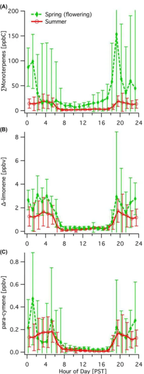
Figure 5.Seasonal comparison of diurnal concentration patterns for (A)total monoterpenes,(B)1-limonene, and(C)p-cymene, shown with standard deviations. The seasonal comparison of1-limonene andp-cymene concentrations demonstrates similar seasonal abun-dances that are slightly higher during flowering.

forest (Bouvier-Brown et al., 2009). 1-limonene was the most prevalent monoterpene observed in the summer and its diurnal patterns and interquartile concentrations were sim-ilar but slightly higher in the spring (Fig. 5b, Table 3). p -Cymene is a known aromatic emitted from (non-flowering) plants with a wide variety of sources and a few minor an-thropogenic sources (e.g., gasoline). Similar to1-limonene, Fig. 5c shows that it was similar between the two seasons both in prevalence and diurnal pattern. The potential anthro-pogenic contribution top-cymene is negligible given the rel-atively low concentrations of dominant gasoline tracers. The relatively comparable concentrations of several

monoter-penes during the two measurement periods in the orange or-chard imply similar emission rates during those two periods.

3.4 Transport of biogenic emissions in the San Joaquin Valley

The relative magnitude of biogenic versus anthropogenic emissions and compound concentrations vary depending on location in the San Joaquin Valley as shown by the compar-ison of the Bakersfield and Lindcove sites (Fig. 6). Given the geographic distribution of agriculture and urban areas in the San Joaquin Valley, the transport of biogenic emis-sions from more vegetated areas is important, and can af-fect atmospheric reactivity and secondary pollutant forma-tion throughout the valley (Rollins et al., 2012; Shilling et al., 2013).

We devised a technique to demonstrate the transport and photochemical processing of primary biogenic emissions in the San Joaquin Valley using the dynamic behavior of several pairs of monoterpenes measured in Bakersfield at the south-ern end of the valley. We compared their ratios over∼700 samples to examine the importance of aging by the three pri-mary atmospheric oxidants (OH, O3, NO3). Each

monoter-pene measured at Bakersfield reacts at different rates with each oxidant, and so by picking monoterpene pairs appropri-ately, we determined the most important oxidants for aging and their timescales (e.g., lifetime = 1/(kOH[OH])).

A comparison of1-limonene toα-pinene shows a distri-bution of ratios (Fig. 7). While some of this variability is possibly due to differences in emissions, it is evident that aging is playing an important role in the variability of ob-served ratios. 1-limonene reacts faster thanα-pinene with all three atmospheric oxidants, but given the average concen-trations of the oxidants, OH oxidation is the fastest and will have the strongest influence on the observed ratios. We used 24 h oxidant average concentrations of 0.25 pptv, 41 ppbv, and 0.29 pptv for OH, O3, and NO3, respectively, at the

Bak-ersfield site based on observations (with steady-state calcu-lations for NO3) and literature values (Bouvier-Brown et al.,

2009; Brown et al., 2009; Rollins et al., 2012). A comparison of1-limonene top-cymene (Fig. S3) similarly demonstrates the importance of aging by OH as the differences in reaction rates are more pronounced than between1-limonene andα -pinene.

A similar comparison of camphene toα-pinene suggests a constant initial emission ratio from regional sources and infers less pronounced aging by ozone and nitrate radicals (Fig. 7b). The observed variability is less dramatic than the other monoterpene pairs and likely due to O3and NO3, given

Figure 6. Diurnal patterns of the sum of biogenic compounds predominantly from agriculture (larger than isoprene) vs. anthropogenic compounds from motor vehicles (including emissions from service stations) at the(A)Lindcove orange orchard site in the spring and(B) the urban Bakersfield site (biogenic compounds are largely monoterpenes).(C)A comparison of motor vehicle compound concentrations between the Bakersfield and Lindcove site shows similar daytime levels, but nighttime and morning values vary due to the buildup of local emissions in the nocturnal boundary layer.

reporting the presence of nitrate chemistry and also a study showing the dominance of OH oxidation of biogenic com-pounds (Rollins et al., 2012; Donahue et al., 2012).

It is evident from this analysis that the observed biogenic compounds are emitted within several hours of transport to the site, which can inform our exploration of the spatial dis-tribution of emissions. Using the FLEXPART footprint mod-eling method (Gentner et al., 2014), we report the spatial dis-tribution of biogenic sources that emit monoterpenes, which advect to the Bakersfield ground site. Figure 8 shows the dis-tribution for the sum of monoterpenes over 6 h of transport, and Fig. S4 shows the distribution of individual chemical species. While many of the compounds appear to have sim-ilar sources in the San Joaquin Valley, some areas are larger emitters of different monoterpenes. The spatial distribution of monoterpene emissions observed in Bakersfield appears to be consistent with the location of croplands (Fig. S1), with

agriculture to the northwest and east/southwest having the greatest area of influence. Yet influence from natural veg-etation is expected, especially in the case of areas near or in the mountains with pine trees and other significant natu-ral emitters of monoterpenes. While the emission distribu-tion presented in Fig. 8 is mostly bounded to the valley floor, emissions from natural vegetation are potentially represented by areas in the foothills/mountains along the southern to east-ern borders of the valley. Furthermore, natural vegetation sur-rounding the valley is a large source of reactive organic car-bon emissions (Karl et al., 2013) and likely plays an impor-tant role in secondary polluimpor-tant formation, especially when mixed with anthropogenic NOx emissions (Shilling et al.,

Observations of monoterpene pairs at the Bakersfield site. (A)Δ-limonene Figure 7.Observations of monoterpene pairs at the Bakersfield site. (A)1-limonene vs.α-pinene. Ratios of lifetimes to all three atmo-spheric oxidants show faster processing of1-limonene. Given the concentrations of radicals, OH oxidation has the fastest timescales and the importance of OH oxidation is also indicated by the most aged parcels coinciding with PAR (representative of OH produc-tion).(B)A comparison ofα-pinene vs. camphene at Bakersfield shows evidence of aging by O3 and NO3 asα-pinene and cam-phene’s lifetimes to OH are identical.

3.5 Impacts on air quality

The principal motivation for studying biogenic emissions from agriculture was to improve our understanding of the im-pact of biogenic emissions on air quality in the San Joaquin Valley. Terpenoid compounds are known to be very reactive and have the potential to form both tropospheric ozone and SOA. Our work has highlighted orange trees as large emit-ters, but many other crops have been shown in this and other studies to have non-negligible emissions (Winer et al., 1992). Previous work has concluded that emissions from agricul-tural croplands are minor (Lamb et al., 1987). This may be

Figure 8.Spatial distribution of monoterpene sources in the south-ern San Joaquin Valley shown using the statistical source footprint of the sum of monoterpenes over 6 h of transport prior to arrival at the CalNex ground site in Bakersfield, CA.

true for some crop types, particularly with respect to the iso-prene emissions. However, the extent of land coverage and leaf mass, together with the range of observed emission fac-tors for all compound classes, is likely to result in croplands representing a significant fraction of biogenic emissions in agricultural regions.

3.5.1 Relative magnitude of biogenic vs. anthropogenic emissions

(e.g.,m/p-xylene, isooctane) between the two seasons shows that nighttime concentrations are similar, but daytime con-centrations of motor vehicle emissions are ∼30 % lower. This is likely due to a combination of enhanced photochem-ical processing and increased dilution during the summer months, when the top of the mixed boundary layer is gen-erally higher. A comparison of diurnal average concentration ranges between sources shows that the summertime sum of monoterpenes (1–19 ppbC, Fig. 5a) was slightly lower than the springtime anthropogenic vehicular contribution (14– 46 ppbC, Fig. 6b). Together the results in this paper suggest that in rural parts of the San Joaquin Valley, anthropogenic emissions from motor vehicles will be slightly higher or the same order as summertime biogenic emissions of terpenoids. During citrus tree flowering, the mass of observed bio-genic compounds was on average 14 times that of in-ferred anthropogenic compounds from vehicular emissions at the Lindcove site. In contrast, the mass of anthropogenic contributions from motor vehicles was 48 times the ob-served monoterpenoids from biogenic sources in Bakersfield (Fig. 6). Contributions from isoprene or oxygenated VOCs from biogenic sources will slightly reduce this difference at Bakersfield, but are not included as these emissions cannot be attributed to agriculture.

Daytime monoterpene concentrations (i.e., sum of speci-ated monoterpenes measured via GC/MS) measured at Lind-cove during spring were on average 6±1 times concentra-tions in the summer. When considering potential differences in meteorological dynamics, this is largely consistent with observations from yearlong PTR-MS measurements at the Lindcove site that reported a 10-fold increase in the monoter-pene BEF between the flowering and non-flowering periods (Fares et al. 2012a). Given that the concentration of quanti-fied flowering compounds in this work was 4 times the sum of monoterpenes (Fig. 2), in total flowering increases carbon emissions∼30-fold, with the non-monoterpene source pro-file for flowering shown in Table 6. This difference in emis-sions between flowering and non-flowering plants needs to be considered in emissions and air quality modeling, since the chemistry of the atmosphere may be significantly differ-ent during flowering periods. Such seasonal evdiffer-ents should be taken into account to accurately model the large changes in biogenic emissions from agriculture and air quality in the San Joaquin Valley. Important emission events include spring flowering, pruning, harvesting, and fertilizer applica-tion (Fares et al., 2012a). During these events large increases in emissions of terpenoids were measured (monoterpenes, sesquiterpenes, and oxygenated terpenes). It is important to note that many agricultural regions, like the San Joaquin Val-ley, are comprised of a diverse mixture of crop types. These plants have different phonological and management cycles, meaning that emission events, such as flowering, will occur at different times and there is less likely to be a singular burst in emissions. The timing and intensity of these events will

have to be determined for each major crop type in a region of interest.

3.5.2 Ozone formation potential

To assess the ability of agricultural terpenoid emissions and flowering events to impact air quality via the contributions of reactive precursors to ozone and SOA, we developed metrics to compare them to motor vehicle emissions. The ability of a compound to produce ozone is quantified through the use of literature MIR values [gO3g−1 compound] (Carter, 2007).

We use MIR to compare sources on a similar basis despite differences in NOx availability as the San Joaquin Valley

has a complex spatial distribution of emissions and meteorol-ogy. Gasoline exhaust, diesel exhaust, and non-tailpipe emis-sions have MIR ozone formation potentials (OFPs) of 4.5, 2.5, and 2.0 gO3g−1, respectively (Gentner et al., 2013). For

the monoterpene profile observed during the spring (includ-ingp-cymene), the OFP was calculated to be 4.1 gO3g−1.

The flowering source profile in Table 6 has an OFP of 4.3– 5.5 gO3g−1with the range of potential values for unknown

values determined from compounds with similar structures and general values provided with the framework. Linalool, which comprises 70 % of the flowering profile, has a known OFP of 5.4 gO3g−1. These calculated values infer that per

mass of emissions, the biogenic emissions have a greater ability to produce ozone than gasoline emissions. This effect may be slightly reduced as terpenoids are generally more re-active with ozone and will also act as a loss mechanism for tropospheric ozone. Overall, we observed that crops are rela-tively minor emitters of isoprene, a highly effective ozone precursor. Emissions of isoprene from natural vegetation, such as oak trees in the foothills surrounding the San Joaquin Valley, play an important role in ozone formation and must also be considered in modeling efforts.

3.5.3 Secondary organic aerosol formation potential Predicting the exact SOA yields and formation from flowering-related compounds is not feasible given the high level of uncertainty associated with predicting SOA yields for these compounds, as many of them have barely been studied. However their potential to form SOA can be ap-proximated using average oxidant concentrations and liter-ature on well-characterized1-limonene andα-pinene yields from OH oxidation and ozonolysis experiments (Saathoff et al., 2009; Kim et al., 2012), and work by Ng et al. (2006) that compares a suite of terpenoid compounds including1 -limonene andα-pinene. SOA yields from1-limonene and

α-pinene range from 0.25 to 0.35 and 0.1 to 0.2 gOA g−1, respectively, for ozonolysis at an organic particle loading of 10 µg m−3 (Saathoff et al., 2009). SOA yields from OH oxidation under high-NOxconditions at similar particle

(Kim et al., 2012). Given the lifetimes to OH and O3

pre-sented in this work, we calculate overall SOA yields of 0.1 and 0.05 gOA g−1 _{at OA = 10 µg m}−3_{. Atmospheric}

oxida-tion in low-NOxconditions will result in higher SOA yields,

but here we restrict the comparison against other sources to the high-NOx conditions observed in the San Joaquin

Val-ley. During the summer, monoterpene emissions were domi-nated by1-limonene with a yield of 0.01 gOA g−1. Assess-ing the behavior of other monoterpenoids associated with flowering and their reaction rates with OH and O3suggests a

slightly lower SOA yield forβ-myrcene (0.04) thanα-pinene and an SOA yield for linalool under 0.01. Overall, under similar loadings, the monoterpene emissions have a greater SOA yield than gasoline exhaust (0.023±0.007 gOA g−1), but lower than diesel exhaust (0.15±0.07 gOA g−1_{) (based}

on the yields for gasoline and diesel derived in Gentner et al., 2012). Estimating SOA yields for the benzenoids as-sociated with flowering is much more difficult given the uncertainties, but SOA yields for C7−8 aromatics in

Gen-tner et al. (2012) were approximately 0.05 gOA g−1for OH oxidation at an organic particle loading of 10 µg m−3 and high-NOx. So for this comparison, we conservatively

as-sume a value of 0.05 gOA g−1or greater for benzenoid com-pounds given their decreased initial volatility due to initially present functional groups. However, recent exploratory work on SOA produced from aqueous processing of phenolic com-pounds reported high SOA yields (Sun et al., 2010). In gen-eral, this work identifies the critical research needed to im-prove estimates of SOA yields from the biogenic compounds discussed in this study through theoretical or experimental studies.

3.5.4 Overall comparison in San Joaquin Valley Detailed modeling using spatially resolved chemical models coupled with emissions will be necessary to fully understand the relative impact of biogenic emissions on air quality using the new information derived in this study. Here we use this information and the case study of the San Joaquin Valley in a back-of-the-envelope calculation to demonstrate the need for further modeling based on the magnitude of emissions from agricultural crops and their potential ozone and SOA. Spatial distribution of emissions and chemistry are essen-tial to account for transport and NOx emissions/chemistry,

but the objective here is to inform the necessity of that fu-ture research. The work presented here focuses on emissions of monoterpenoids and larger compounds, and does not in-clude isoprene or small oxygenated VOCs and alcohols that are also emitted from vegetation. As the focus is on the rel-ative impacts of agriculture, we do not consider the poten-tial transport of emissions from natural vegetation (e.g., pine trees, oak trees) in the foothills or mountains. We use avail-able metrics from the literature to assess potential ozone and SOA formation with the caveat that they may not fully cap-ture the differences in NOxavailability and thus the

chemi-Figure 9.The components of the net ozone flux for the Lindcove or-ange orchard.(A)Modeled fluxes of monoterpenes and floral com-pounds are greatest in the spring during flowering, but are signifi-cant throughout the summer. Sesquiterpene emissions are assumed to be equivalent to monoterpene emissions.(B)Ozone formation and deposition fluxes per acre throughout the year show variable ozone formation with more constant deposition (stomatal and chem-ical). Formation is calculated as potential O3(i.e., assuming a VOC-limited regime).(C)The combined effect of these fluxes produces a net flux into the canopy except when biogenic emissions are high.

cal regimes between urban and rural areas in the valley. It is with these caveats that we estimate the magnitude of emis-sions from agricultural vegetation relative to motor vehicles and their potential to impact air quality.

Based on fuel sales for the valley and the results of Gentner et al. (2012, 2013), gas-phase gasoline ex-haust emissions are 1.8×108 g day−1, non-tailpipe gaso-line emissions are 4.6×107g day−1, and diesel emis-sions are 4.6×107g day−1. Together this amounts to 2.7×108g day−1 _{and an ozone formation potential of}

1.0×109gO3day−1, with the reactivity dominated by

gaso-line sources. Using the SOA yields from Gentner et al. (2012), potential SOA from motor vehicles is 8.0×106 gOA day−1(Table 8).

Table 8.Metrics of secondary pollutant formation, emissions, and potential impacts of biogenic emissions from agricultural crops compared to motor vehicles in California’s San Joaquin Valley.

Ozone formation SOA yield Emission estimates Potential production

Potential [gOA g−1] for SJV Ozone SOA

[gO₃g−1] [10−7×g d−1] [10−8×gO₃d−1] [10−6×gOA d−1]

Agriculture: monoterpenes 4.1 ∼0.1 1–30a 0.6–12 1–30

Agriculture: flowering compounds 4.3–5.5 ∼0.03b 24–720c 10–400 7.2–220

Gasoline exhaustd 4.5 0.023±0.007 18 8.0 2.7

Non-tailpipe gasoline emissions 2.0 0.0024±0.0001 4.6 0.93 0.1

Diesel exhaustd 2.5 0.15±0.07 4.6 1.2 5.1

References: vehicular ozone formation potential values are MIR values from Gentner et al. (2013a). a_{Range is set as BEF = 80–3000 ngC gDM}−1_h−1_.

b_{SOA yield for flowering is lower estimate assuming a conservative yield of 0.05 for unstudied aromatics. Linalool (44 % of flowering source profile) has a very low SOA yield as well} (0.007).

c_{Estimated as 24 times baseline monoterpene emissions, and would also be accompanied by a factor of 5 increase in monoterpene emissions.}

d_{Both gasoline and diesel exhaust include products of incomplete combustion (excluded in SOA calculations per Gentner et al. (2012)) and gasoline exhaust also includes cold start} emissions (estimated as equivalent to 60 % of gasoline running exhaust (Gentner et al., 2013a)).

Figure 10. (A)Ambient ozone data since 1987 (CARB) show ex-ceedances above 75 ppbv at both the center of the valley and down-wind in the Sierra Nevada with the primary period of concern from day 70 to 320. No trends were apparent in the data from 1987 until present.(B)The weekly net effect of the orange orchard on ozone over this period is shown to be a net source of ozone in the spring-time during flowering, and relatively neutral for most of the summer until the fall, when it becomes a sink.

of 85 cm2g−1 and a canopy leaf area index of 3.0 m2 leaf area m−2 land area (Fares et al., 2012b). These leaf mass density and leaf area factors are derived from the orange orchard, and are applied here with caution to the diversity of crops found in the valley. This range of estimates in-cludes the summertime BEF measured in the orange orchard (0.13 nmol m−2_s−1_{) (Fares et al., 2012a). We assume a}

to-tal land cover by agriculture of 3 million acres in the San Joaquin Valley (Table 1).

In terms of total mass from agricultural sources, base-line monoterpene emissions are estimated to be on the same order as anthropogenic sources, with a range of 0.1–3×108g day−1. The CARB emission inventory of 1.8×107g monoterpenes day−1from agriculture in the San Joaquin Valley is at the low end of our estimated range. Our estimated emission factor is a lower limit since it does not in-clude sesquiterpenes or emissions during flowering or other emission events, which may increase emissions by a factor of 30 or at least 2, respectively, with the timing depending on the diversity of crop types and management practices.

With regards to the production of ozone from organic pre-cursors, monoterpene emissions from agriculture have the ability to produce 0.6–12× 108gO3day−1, making them

equally important as organic emissions from motor vehicles, but further analysis with NOxsensitivity is essential to

eluci-date the relative importance for the region. As this is a base-line value, it is evident that emissions occurring during flow-ering will have a major impact on ozone production given the substantial increase in emissions, and additional consid-erations for sesquiterpene emissions will increase ozone pro-duction as well.

Estimating SOA has a significant amount of uncertainty associated with it, but for comparison with motor vehicles we estimate that monoterpene emissions from agriculture can contribute 1–30×106gOA day−1, across the range of emis-sions and SOA yields (at 10 µg m−3_{). This means that}

vehicles (8.0×106gOA day−1_{) to produce SOA, which does}

not include sesquiterpene emissions or other emission events such as flowering. The valley-wide magnitude of flower-ing emissions is highly uncertain and warrants further work. Rough estimates with a range of flowering emissions are given with potential ozone and SOA formation in Table 8.

3.5.5 Citrus: a case study on the net effect of agricultural crops on ozone uptake and formation

Many woody plants, including orange trees, remove some ozone from the ambient atmosphere via uptake through their stomata. This process, stomatal deposition, along with soil/plant surface deposition and the reaction of ozone with reactive biogenic compounds in the air produces a flux of ozone into the plant canopy, which was measured for a full year at the Lindcove field site. Chemical deposition via reac-tion with biogenic volatile organic compounds (BVOCs) was estimated to be 10–26 %, while stomatal deposition and soil deposition were each responsible for approximately∼30 % of ozone losses (Fares et al., 2012b). A full discussion of these fluxes and their partitioning into different mechanisms has been published in Fares et al. (2012b).

To determine the net effect of the orange orchard on re-gional ozone, we compared the measured ozone flux into the canopy with the amount of ozone likely to be produced downwind based on emissions and OFP values. Monoter-pene BEFs from the field site for spring and summer were used from Fares et al. (2012a), with the summer flux mul-tiplied by 2 during non-flowering emission events (harvest, pruning, fertilizer application) when emissions measured by PTR-MS exceeded modeled emissions. Based on the work of Ormeno et al. (2010), sesquiterpene emissions were assumed to be equivalent to monoterpene emissions and were assumed to have an OFP of 4 gO3g−1 based on the range of

poten-tial OFPs. Emissions of floral compounds during the spring flowering period were estimated by multiplying monoterpene emissions by 4.0 per the results of Fig. 2. Additionally, down-wind chemical removal of ozone beyond the measured flux reported previously (Fares et al., 2012b) was accounted for using the monoterpene emissions and the probability of re-action with ozone. Figure 9 summarizes the results of this analysis with total emissions, ozone fluxes into the canopy, ozone production, and the net effect. The net effect on a weekly timescale of these processes is shown in Fig. 10 over the period of ozone exceedances in the region. The orchard is a net source of ozone in the springtime during flower-ing, and is neither a major source nor sink for most of the summer. The orchard is a sink in the fall and in the early spring before flowering begins. Given that flowering occurs at different times for different crops throughout the valley, net ozone production during flowering may not translate to a valley-wide effect. The effect of ozone deposition was not in-cluded in the basin-wide comparison of agriculture to motor

vehicles (Sect. 3.5.4) as exhaust emissions contain significant amounts of alkenes that can also remove ozone initially.

3.5.6 Implications

This work has demonstrated the importance of biogenic or-ganic carbon emissions from agricultural crops relative to ve-hicular emissions in terms of total emissions and the forma-tion of ozone and SOA in the San Joaquin Valley. Further highly resolved modeling of emissions and chemistry is war-ranted based on this new information. Recent work examined flowering emissions in the urban area of Boulder, CO, and temporarily incorporated flowering into the MEGAN model (Baghi et al., 2012). The study concluded the impacts of flowering in Boulder, CO, were minor (equivalent to 11 % of the monoterpene flux). Our results suggest a larger annual temporary impact of flowering in agricultural regions with high densities of flowering foliage, but it is dependent on the composition of crops and flowering timing. When the mag-nitude of the flowering event is considered across a region, it may have a substantial effect on the biogenic emission in-ventory and likely on atmospheric composition and air qual-ity, especially in regions prone to air quality problems. Or-ange tree flowering lasted for approximately one month, but the duration of flowering varies between plant species. It is important to note that most of the flowering occurs in the spring, conveniently before the greatest frequency of ozone exceedances in the San Joaquin Valley during summer, when contributions to ozone precursors would be more important.

The newly characterized compounds in this study should be included in the MEGAN and BEIGIS models since their emissions during flowering were on the same order as or greater than all the terpenoids observed. Further work is nec-essary to better characterize the basal emission factors, de-pendent parameters, and, in the case of the novel compounds, their ozone and SOA formation potential. Emissions due to flowering and other seasonal events need to be assessed for other major crops, and possibly natural vegetation. The mod-eling of biogenic emissions from agriculture has a major ad-vantage over natural vegetation: the ability to gain more de-tailed information on the composition of vegetation species. These data, along with emission factors, provide the neces-sary components to more regional emissions and potentially identify potential regional changes in emissions with shifts or rotations in crop plantings.