CLASSIFICAÇÃO MULTIMODAL EM IMAGENS
EDEMIR FERREIRA DE ANDRADE JUNIOR
CLASSIFICAÇÃO MULTIMODAL EM IMAGENS
DE SENSORIAMENTO REMOTO
Dissertação apresentada ao Programa de Pós-Graduação em Ciência da Computação do Instituto de Ciências Exatas da Univer-sidade Federal de Minas Gerais como re-quisito parcial para a obtenção do grau de Mestre em Ciência da Computação.
Orientador: Jefersson Alex dos Santos
Coorientador: Arnaldo de Albuquerque Araújo
Belo Horizonte
EDEMIR FERREIRA DE ANDRADE JUNIOR
MULTIMODAL CLASSIFICATION OF REMOTE
SENSING IMAGES
Dissertation presented to the Graduate Program in Computer Science of the Fede-ral University of Minas Gerais in partial ful-fillment of the requirements for the degree of Master in Computer Science.
Advisor: Jefersson Alex dos Santos
Co-Advisor: Arnaldo de Albuquerque Araújo
Belo Horizonte
c
2016, Edemir Ferreira de Andrade Junior. Todos os direitos reservados.
Ferreira de Andrade Junior, Edemir
D1234p Multimodal Classification of Remote Sensing Images / Edemir Ferreira de Andrade Junior. — Belo Horizonte, 2016
xx, 66 f. : il. ; 29cm
Dissertação (mestrado) — Federal University of Minas Gerais
Orientador: Jefersson Alex dos Santos
1. Data Fusion. 2. Remote Sensing. 3. Multimodal Classification. I. Jefersson Alex dos Santos. II. Título.
“Your spirit is the true shield.” (Morihei Ueshiba, The Art of Peace - 1992)
Resumo
Sistemas de Informação Geográfica (SIGs) são ferramentas de computador que ana-lisam, armazenam, manipulam e visualizam informações geográficas em mapas. Per-mitindo às pessoas mais facilmente verem, interpretarem e entenderem os padrões e relacionamentos, os SIGs são importantes ferramentas que ajudam a tomar decisões em diversas questões relacionadas às políticas públicas de monitoramento ambiental e urbano. Além disso, são instrumentos essenciais para o planejamento do desen-volvimento econômico e da análise das atividades de agricultura e extração mineral. Nesse contexto, Imagens de Sensoriamento Remoto (ISRs) têm sido usadas como uma das mais importantes fonte de dados, principalmente com relação à criação de mapas temáticos. Esse processo é geralmente modelado como um problema de classificação supervisionada em que o sistema precisa aprender os padrões de interesse fornecidos pelo usuário e atribuir uma classe ao restante das regiões da imagem. Associados à natureza das ISRs, existem vários desafios que podem ser ressaltados: (1) são imagens georreferenciadas, ou seja, existe uma coordenada geográfica associada à cada pixel da imagem; (2) os dados comumente captam frequências específicas em todo o espectro eletromagnético em vez de apenas o espectro visível, o que exige o desenvolvimento de algoritmos específicos para descrever os padrões; (3) o nível de detalhe de cada imagem pode variar, resultando em imagens com diferentes resoluções espacial e de pixel, porém cobrindo a mesma área de interesse; (4) devido às imagens de alta res-olução de pixel, algoritmos de processamento eficientes são desejáveis. Assim, é muito frequente ter imagens obtidas a partir de diferentes sensores, o que poderia melhorar a qualidade dos mapas temáticos gerados. No entanto, isso exige a criação de téc-nicas capazes de codificar e combinar adequadamente as diferentes propriedades das imagens. Desse modo, esta dissertação propõe duas novas técnicas de classificação de regiões em ISR, com a habilidade de codificar características extraídas de diferentes sensores, dos domínios espacial e espectral. O principal objetivo é o desenvolvimento de um arcabouço capaz de explorar a diversidade entre esses diferentes tipos de dados para alcançar alta acurácia na criação de mapas temáticos. A primeira abordagem
posta, chamada de Voto Majoritário Dinâmico, combina dados de diferentes domínios usando uma estratégia de fusão de dados no nível de decisão que explora a especiali-dade de diferentes classificadores e realiza a combinação deles para a decisão final de cada pixel na construção do mapa temático. Essa abordagem foi criada para lidar apenas com problemas multi-classe e foi avaliada em uma base de dados de cobertura de um cenário urbano. A segunda abordagem proposta realiza a combinação de dados nos três níveis fusão: pixel, características e decisão, assim explorando diferentes tipos de características, extraídas de diferentes sensores usando uma estratégia baseada em boostingde classificadores. Diferentemente do Voto Majoritário Dinâmico, esse método foi projetado para lidar com problemas binários e multi classe, e avaliado na mesma base de dados multi classe em cenário urbano, mas também no problema binário para reconhecimento de plantações de café.
Palavras-chave: Classificação Multimodal; Sensoriamento Remoto; Fusão de Dados.
Abstract
Geographic Information Systems (GIS) are computer-based tools that analyze, store, manipulate, and visualize geographic information on maps. Enabling more easily people to see, interpret, and understand patterns and relationships, they are important tools, which help to make decisions on diverse issues related to public policies of urban and environmental monitoring. Furthermore, they are essential tools for economic development planning and analysis in activities of agriculture and mineral extraction. In this context, Remote Sensing Images (RSIs) have been used as a major source of data, particularly with respect to the creation of thematic maps. This process is usually modeled as a supervised classification problem where the system needs to learn the patterns of interest provided by the user and assign a class to the rest of the image regions. Associated with the nature of RSIs, there are several challenges that can be highlighted: (1) they are georeferenced images, i.e., a geographic coordinate is associated for each pixel; (2) the data commonly captures specific frequencies across the electromagnetic spectrum instead of the visible spectrum, which requires the development of specific algorithms to describe patterns; (3) the detail level of each data may vary, resulting in images with different spatial and pixel resolution, but covering the same area; (4) due to the high pixel resolution images, efficient processing algorithms are desirables. Thus, it is very common to have images obtained from different sensors, which could improve the quality of thematic maps generated. However, this requires the creation of techniques to properly encode and combine the different properties of the images. Thus, this dissertation proposes two new techniques for classification of regions in remote sensing images that manage to encode features extracted from different sources of data, spectral and spatial domains. The major objective is the development of a framework able to exploit the diversity of these different types of features to achieve high degrees of accuracy in the creation of thematic maps. The first approach proposed, named Dynamic Majority Vote, combines the data from different domains using a strategy of fusion at the decision level, which exploits the specialty of different classifiers and combines them for a final
decision for each pixel in the thematic map. This approach was created to handle only with multiclass problems and was evaluated in an urban land cover scenario dataset. The second approach proposed is a combination of the pixel, feature and decision level fusion, which exploits different types of features, extracted from various sensors using a boosting-based approach. Differently of the Dynamic Majority Vote, this method can handle with binary and multiclass problems, and was evaluated in a multiclass urban scenario dataset, and also in a binary coffee crop recognition problem.
Keywords: Multimodal Classification; Remote Sensing; Data Fusion.
List of Figures
1.1 An illustration of multimodal data acquisition . . . 2
2.1 An illustration of the active and passive sensors . . . 8
2.2 An example of thematic map resulted by a classification algorithm . . . 9
2.3 Bad segmentation in concern of supervised evaluation . . . 10
2.4 IFT-Watergray on different segmentation level . . . 11
2.5 An illustration of region-based feature extraction in the visible domain im-age. The input image is segmented in several regions, and for each region is computed a feature vector using different region descriptors. . . 13
2.6 An illustration of feature extraction at multi/hyper spectral image . . . 14
2.7 An example of space projection using the Principal Component Analysis and Linear Discriminant Analysis . . . 16
2.8 An illustration of resampling of images using the nearest neighbor assignment 17 2.9 An illustration of resampling of regions using the nearest neighbor assignment 17 2.10 An illustration of Adaboost iterations. . . 21
2.11 Complementarity between optical and SAR sensors . . . 23
2.12 Mixture of pixels in a optical image . . . 24
2.13 An illustration of a Pansharpening process . . . 27
3.1 Base framework used in both strategies proposed . . . 32
3.2 The Proposed Dynamic Weight Matrix (DWM)-based framework . . . 34
3.3 An example of the construction of Dynamic Weight Matrix (DWM), regard-ing to the class 1 . . . 37
3.4 How to use the Dynamic Weight Matrix . . . 38
3.5 The Proposed Boosting-based approach framework . . . 40
3.6 How to use the Boosting-based approach . . . 43
4.1 Urban Dataset - IEEE GRSS Data Fusion Contest 2014 . . . 46
4.2 Intravariance class challenge in Dataset - Coffee Crop Recognition . . . 48
4.3 Dataset - Coffee Crop Recognition . . . 49 4.4 Dynamic majority vote results . . . 52 4.5 Comparison thematic maps: Dynamic Majority Vote and Majority Vote . . 54
List of Tables
3.1 Notations . . . 33
4.1 General Information - Train Set. . . 47
4.2 General Information - Test Set. . . 47
4.3 Distribution of Pixels per Class. . . 47
4.4 General Information - Train Set. . . 48
4.5 Distribution of Pixel per Class - Coffee Crop Recognition. . . 49
4.6 An Example of a Confusion Matrix with 3 class . . . 49
4.7 Kappa Index in Urban Dataset - Boosting-based Approach. . . 55
4.8 Accuracy in Urban Dataset - Boosting-based Approach. . . 55
4.9 Accuracy and Kappa Index in Crop Coffee - Boosting-based Approach . . 56
Contents
Resumo xi
Abstract xiii
List of Figures xv
List of Tables xvii
1 Introduction 1
1.1 Motivation . . . 1
1.2 Objective and Contributions . . . 3
1.3 Organization of the Text . . . 4
2 Related Work and Background 7 2.1 Remote Sensing . . . 7
2.2 Segmentation . . . 8
2.3 Feature Extraction . . . 12
2.3.1 Spatial Domain Representation . . . 12
2.3.2 Spectral Domain Representation . . . 14
2.3.3 Mapping Between Domains . . . 15
2.4 Supervised Learning . . . 18
2.5 Data Fusion . . . 22
3 Methodology 31 3.1 Dynamic Majority Vote . . . 31
3.1.1 Object Representation . . . 35
3.1.2 Feature Extraction . . . 35
3.1.3 Training . . . 35
3.1.4 Dynamic Weight Matrix Construction . . . 35
3.1.5 Predicting . . . 37
3.2 Boosting-Based Approach . . . 38
3.2.1 Object Representation . . . 39
3.2.2 Feature Extraction . . . 39
3.2.3 Training . . . 40
3.2.4 Predicting . . . 42
4 Experimental Analysis 45 4.1 Datasets . . . 45
4.1.1 Urban Land-Cover . . . 45
4.1.2 Coffee Crop Recognition . . . 47
4.2 Evaluation metrics . . . 49
4.3 Dynamic Majority Vote Approach . . . 50
4.3.1 Setup . . . 50
4.3.2 Results and Discussion . . . 51
4.4 Adapted Boosting Approach . . . 53
4.4.1 Setup . . . 53
4.4.2 Results and Discussion . . . 55
5 Conclusions and future work 57
Bibliography 59
Chapter 1
Introduction
1.1
Motivation
Over the years, there has been a growing demand for remotely-sensed data. Specific objects of interest are being monitored with earth observation data, for the most varied applications. Some examples include ecological science [Ghiyamat and Shafri, 2010], hydrological science [Schmid et al., 2005], agriculture [Lanthier et al., 2008], military [Briottet et al., 2006], and many other applications.
Remote sensing images (RSIs) have been used as a major source of data, par-ticularly with respect to the creation of thematic maps. A thematic map is a type of map that displays the spatial distribution of an attribute that relates to a particular theme connected with a specific geographic area. This process is usually modeled as a supervised classification problem where the system needs to learn the patterns of interest provided by the user and assign a class to the rest of the image regions.
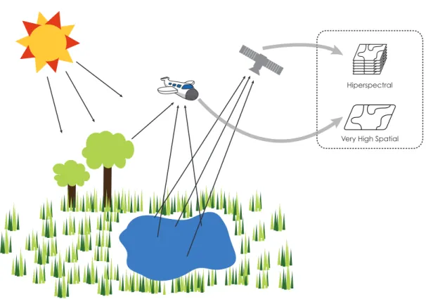
In the last few decades, the technological evolution of sensors has provided re-mote sensing analysis with multiple and heterogeneous image sources (Figure 1.1), which can be available for the same geographical region: high spatial, multispectral, hyperspectral, radar, multi-temporal, and multiangular images can today be acquired over a given scene.
Typically, these sensors are designed to be specialists in obtaining one or few properties from the earth surface. This occurs because each sensor, due to technical and cost limitations, has a specific observation purpose and operate at different wave-length ranges to achieve it. Since the sensors are specialists, they carry different and complementary information, which can be combined to improve classification of the materials on the surface and consequently increase the quality of the thematic map. In this scenario, it is essential to use a more suitable technique to combine the different
2 Chapter 1. Introduction
Hiperspectral
Very High Spatial
Figure 1.1: An illustration of multimodal data acquisition. The figure shows two different platforms: a plane and a satellite; carrying sensors which extract different information (spectral and spatial) over the same region, creating a multimodal per-spective.
features in an effective way.
The remote sensing community has been very active in the last decade in propos-ing methods that combine different modalities [Gomez-Chova et al., 2015]. In addition to support the research on this important topic, every year since 2006, the IEEE Geoscience Remote Sensing Society (GRSS) has been developing a Data Fusion Con-test (DFC), organized by the Image Analysis and Data Fusion Technical Committee (IADFTC), which aims at promoting progress on fusion and analysis methodologies for multisource remote sensing data. Also, other data fusion challenges have been proposed more recently by the International Society for Photogrammetry and Remote Sensing (ISPRS), devoted to the development of international cooperation for the advancement of photogrammetry and remote sensing and their applications. All the effort to reach advance in this research area shows the high interest and timely relevance of the posed problems.
1.2. Objective and Contributions 3
no access, e.g., the atmospheric constituents cause wavelength dependent absorption and scattering of radiation, which degrade the quality of images. Second, combining heterogeneous datasets such that the respective advantages of each dataset are maxi-mally exploited, and drawbacks suppressed, is not an evident task. Third, as pointed by [Mura et al., 2014], it is very difficult to conclude what is the best approach for multimodal data fusion, since it depends on the foundation of the problem, the nature of the data used and the source of information utilized.
There are also several research challenges in computational scope when working with remote sensing image classification such as: (1) remote sensing data is inherently big, even at 250 m coarse spatial resolution, MODIS NDVI product can contains more than 20 millions of pixels, jointly with a time series of 5 thousands observations. The most of machine learning models described as state of art (e.g., Deep Neural Networks, non linear Support Vector Machines), cant handle with the magnitude of this data; (2) segmentation scale, accompanied by the large amount of information at the level of object in very high spatial resolution images, the segmentation algorithms have difficulty in defining the optimum scale to be used; (3) pixel mixture and dimensionality reduction, images with high spectral resolution must be pre-processed due to problems such as high dimensionality, treatment of noise and corrupted bands, mixture of pixels due to the low spatial resolution; (4) efficiency, even collecting information from various sensors efficiency and capability to process that amount of data is desired or even crucial depending on the application. In applications such as tsunami or earthquakes, the data must be analyzed in near real time, and the difference of a few seconds can save hundreds or even thousands of lives in a seaquake.
1.2
Objective and Contributions
4 Chapter 1. Introduction
the HS image is analyzed by the spectral signature of each pixel; (3) feature extrac-tion, feature vectors are extracted from the segmented regions of VHS using various descriptors and the spectral signatures are obtained by different dimensionality reduc-tion methods; (4) training, using different learning methods and the feature vectors extracted from both domains a set of base classifiers is created; (5) dynamic weight matrix construction, using the trained base classifiers and a validation set is create a matrix of weights which represents the importance of each classifier at decision in every class; (6) prediction, given unseen samples and built the dynamic weight matrix, a pre-dict for every new sample is made using the weights of the decisions of every classifier at that sample. Our approach has the ability to exploit these classifiers which have a specialty in some specifics classes, but would be suppressed by the other classifiers in an equal weight scheme. The second approach is a boosting-based approach based on the SAMME Adaboost [Zhu et al., 2009]. Such as the Dynamic Majority Vote, the boosting-based approach uses a supervised learning framework, but may be divided in five steps: (1-3) data acquisition, object representation and feature extraction as described in the previous description; (4) training, using the features extracted from both domains and diverse learning methods a set of weak learners is created, which at every boosting iteration once is selected to compose the final strong classifier; (5) prediction, given the unseen samples and the set of selected weak learners, a predict for every new sample is made regarding to the linear combination of the weak learner predictions. In this approach, we exploit the inherent feature selection of the Adaboost for the combination of different modalities, as a natural process.
To summarize, this work has the following two main contributions:
• A late fusion technique, called Dynamic Majority Vote, which exploits the spe-cialty of different classifiers and combines them for a final decision for each pixel in the thematic map;
• A boosting-based approach, capable to combine different modalities using the inherent feature selection of the Adaboost.
1.3
Organization of the Text
1.3. Organization of the Text 5
Chapter 2
Related Work and Background
The creation of a thematic map is usually modeled as a supervised classification prob-lem where the system needs to learn the patterns of interest from samples provided by the user and assign a class to the rest of the image regions. Typically, this process are composed by the following steps: data acquisition, segmentation, feature extraction, and classification.
This chapter starts with some fundamental concepts about remote sensing and data acquisition in Section 2.1. Section 2.2 presents the concepts and a brief review about segmentation at remote sensing classification. Section 2.3 describes the feature extraction in spatial and spectral domains. Section 2.4 presents the concepts of super-vised learning and a literature review of fusion of classifiers in remote sensing. At the end, in Section 2.5, review concepts concerning multisource data are presented.
2.1
Remote Sensing
Among the huge number of definitions for “remote sensing”, Crosta et al. Crosta [1999] presents a scientific and simple definition: “Remote sensing is the science which aims to obtain images from the earth surface through the detection and quantitative mea-surement of the answers of the interaction of electromagnetic radiation with terrestrial materials”.
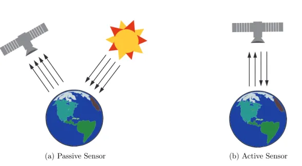
Sensors are define as a device used to detect the electromagnetic radiation re-flected or emitted from an object, which usually is divided in two different types: passive sensors and active sensors (Figure 2.1).
Passive sensors respond to external stimuli, they record natural energy that is reflected or emitted from the Earth’s surface. The most common source of radiation detected by passive sensors is reflected sunlight. In contrast, active sensors use internal
8 Chapter 2. Related Work and Background
(a) Passive Sensor (b) Active Sensor
Figure 2.1: An illustration of the active and passive sensors. (a) A passive sensor receiving electromagnetic radiation emitted by the sun and reflected onto the surface of Earth (b) An active sensor emitting internal stimuli onto the surface of the Earth and receiving it back.
stimuli to collect data about earth. For example, a laser-beam remote sensing system projects a laser onto the surface of Earth and measures the time that it takes for the laser to reflect back to its sensor. The output of a sensor is usually a digital image representing the scene being observed. As a digital image, we refer to the following definition:
Definition 1. A digital imageID
M×N is a discrete representation of a real scene, formed
by M ×N pixels, where each pixel “p” is expressed as a vector xp ∈ ℜD, that explains
some quantitative measurement of a region.
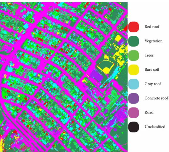
In order to extract useful information from the images, image processing tech-niques can be employed to enhance visual interpretation, and to correct or restore the image of geometric distortion, blurring or degradation among other factors. In many cases, image segmentation and classification algorithms are used to delineate different areas or objects in an image into thematic classes. The resulting product is a thematic map of the study area. An example of a thematic map, covering an urban area, is showed in Figure 2.2.
2.2
Segmentation
2.2. Segmentation 9
Figure 2.2: An illustration of a thematic map resulted by a classification algorithm covering an urban area.
is homogeneous with respect to some property, such as gray value or texture [Pal and Pal, 1993].
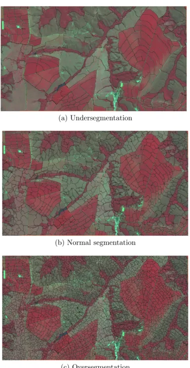
The image segmentation is an important processing step in remote sensing image analysis, since we are interested in specific objects in the image and split up an image into too few (undersegmentation) or too many regions (oversegmentation) can disturb the representation. Therefore, a good performance in segmentation phase is essential for an accurate posterior analysis of the object.
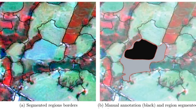
Evaluating the quality of a segmentation method is a subjective task, where a human visually compares the image segmentation results for different segmentation algorithms, and that is a tedious process and inherently limits the depth of evaluation [Zhang et al., 2008]. In some cases, an alternative evaluation is made, so called super-vised evaluation, where a segmented image is compared against a manually-segmented or pre-processed reference image (also limited by manual human work).
10 Chapter 2. Related Work and Background
on remote sensing image is showed in Figure 2.3.
(a) Segmented regions borders (b) Manual annotation (black) and region segmented (gray)
Figure 2.3: An example of a bad segmentation in concern of supervised evaluation. (a) The borders of a remote sensing image, segmented in regions. (b) A comparison of a human manual annotated region (black) and the region segmented by an algorithm (gray).
Over the years, there has been a growing demand for remotely-sensed data, and with the evolution of sensors technology, a considerable quantity of works appeared concerning segmentation in remote sensing images [Zhang et al. [2015], Gaetano et al. [2015], Baumgartner et al. [2015]].
Due to the enormous data and composite details of applications of high-resolution remote sensing image, the methods of segmentation were adapted to handle all this information [Priyadharsini et al., 2014].
In [Dey et al., 2010], the authors performed an extensive review of different image segmentation techniques applied on optical remote sensing images from more than 3000 sources including, journals, thesis, papers, etc. The state of art research on each category was provided with emphasis on developed technologies and image properties used by them.
2.2. Segmentation 11
minima. The method is based on the Image Foresting Transform (IFT) [Falcão et al., 2004], an unified and efficient approach to reduce image processing problems to a minimum-cost path forest problem in a graph. Since we are dealing with large images, the IFT-Watergray is effective, efficient and capable of segmenting multiple objects in almost linear time. Examples of different segmentation levels using the IFT-Watergray are showed in Figure 2.4.
(a) Undersegmentation
(b) Normal segmentation
(c) Oversegmentation
12 Chapter 2. Related Work and Background
2.3
Feature Extraction
The feature extraction at the pixel-level is very common in the field of remote sensing, which relies in assigning each pixel to a semantically or physically meaningful class, taking in account the value of the pixel (or a stack of values in the case of spectral images). In this case, each pixel property is inferred from these values.
Nonetheless, dealing with high spatial resolution images, more than a single pixel value can be explored, opening the possibility to extract different, and complementary information from the interest objects. For instance, pixels belonging from roofs with different sizes but equal pixel values cannot be distinguished from each other without the geometrical information.
Conjointly with the segmentation methods, the region-based approaches grow at the remote sensing classification. Exploring such efficient and faster information extraction methods, high-resolution remote sensing image processing has turned into a significant research theme in remote sensing applications [Priyadharsini et al. [2014], dos Santos et al. [2010]].
In this work, a jointly of the pixel and region-based features was used, regarding with the image domain. We used the region descriptor and feature vector definition proposed in [da Silva Torres and Falcao, 2006]:
Definition 3. A feature vector vr of a region r can be thought of as a point in a ℜn
space vr= (v1, v2, ..., vn), where n is the dimension of the vector.
Definition 4. A simple region image content descriptor (also know, region descriptor)
D is defined as a function fD : r −→ ℜn, which extracts a feature vector vr from a
region r.
2.3.1
Spatial Domain Representation
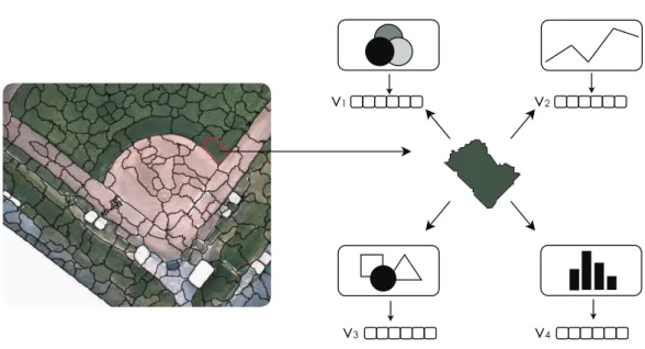
Concerning high spatial resolution images, we have used image descriptors based on visible color and texture information to encode complementary feature. An illustration of region-based features extraction is showed in Figure 2.5.
A brief explanation of each descriptor is showed below:
2.3. Feature Extraction 13
v1 v2
v4
v3
Figure 2.5: An illustration of region-based feature extraction in the visible domain image. The input image is segmented in several regions, and for each region is computed a feature vector using different region descriptors.
• Color Coherence Vector (CCV): This extraction algorithm classifies the im-age pixels in coherent or incoherent pixels. This classification considers if the pixel belongs or not to a region with similar colors, called coherent region. After the classification, two color histograms are computed: one for coherent pixels and another for incoherent pixels. Both histograms are concatenated to compose the feature vector.For more details, see [Pass et al., 1997].
• Color Autocorrelogram (ACC): it maps the spatial information of colors by pixel correlations in different distances. The autocorrelogram computes the probability of finding in the image two pixels with color C in a distance d from each other. After the autocorrelogram computation, there are m probability values for each distance d considered, where m stands for the number of colors in the quantized space. The implemented version quantized the RGB color space into 64 bins and considered 4 distance values (1, 3, 5, and 7). For more details, see Huang et al. [1997].
14 Chapter 2. Related Work and Background
pixels. The two histograms are concatenated and stored into the feature vector. For more details, see [Stehling et al., 2002].
• Unser: This descriptor aims to reduce the complexity of co-occurrence matrices while keeping good effectiveness. Its extraction algorithm computes a histogram of sums Hsum and a histogram of differences Hdif. The image is scanned and,
for each angle a and distance d defined, the histogram of sums is incremented considering the sum and the histogram of differences is incremented considering the difference between the values of two neighboring pixels. As with gray level co-occurrence matrices, measures like energy, contrast, and entropy can be extracted from the histograms. For this work, 256 gray levels and 4 angles were used (0o
, 45o
, 90o
e 135o
), as well as distance d equal to 1.5 and eight different measures were extracted from the histograms. The feature vector was composed by 32 values. For more details, see [Unser, 1986]
2.3.2
Spectral Domain Representation
For the multi/hyper spectral images, due to the low spatial resolution, we exploit di-mensionality reduction/projection methods statistics based on different assumptions, in order to obtain diversity of spectral signatures using a pixel-wise method. An illus-tration of the multi/hyper spectral features extraction is showed in Figure 2.6.
Mixed pixel (vegetation + soil)
Pure pixel (water) Mixed pixel (soil + rocks)
Wavelenght(nm) R eflec tanc e 4000 3000 2000 1000 0
300 600 900 1200 1500 1800 2100 2400
Wavelenght(nm) R eflec tanc e 4000 3000 2000 1000 0
300 600 900 1200 1500 1800 2100 2400
R eflec tanc e 4000 3000 2000 1000 0
300 600 900 1200 1500 1800 2100 2400
Wavelenght(nm)
2.3. Feature Extraction 15
We have used the following algorithms:
• Principal Component Analysis (PCA) [Pearson, 1901]: it is a statistical method that uses a linear transformation (orthogonal) to transform a set of pos-sibly correlated variables into a set of linearly uncorrelated variables called prin-cipal components.
The transformation is defined to create the set of successive orthogonal compo-nents that explains a maximum amount of the variance of the data, in which the first principal component has the largest possible variance and each consec-utive component in turn has the highest variance possible under the constraint that it is orthogonal to the preceding components. The resulting vectors are an uncorrelated orthogonal basis.
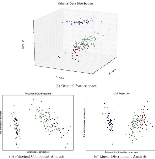
An example of projection realized to a lower dimensional space by PCA is showed in Figure 2.7(b).
• The Fisher Linear Discriminant (FLD)[Fisher, 1936]: Also know as canoni-cal discriminant, is a statisticanoni-cal method used in intent to find a linear combination of features which better separates the data, but considering mainly the classes. The method attempts to find a set of transformed axes that maximizes the ratio of the average distance between classes to the average distance between sam-ples within each class. Since the FLD attempts to model the difference between samples taking in account the classes of the data, it might be more useful for image classification than other methods like PCA, which do not include label information of the data.
An example of a projection space using the Linear Discriminant Analysis (LDA), a special case of FLD, is showed in Figure 2.7(a). The LDA is a particular case which assumes that the conditional probability density functions are normally distributed, share the same covariance matrix, and present covariances with full rank.
2.3.3
Mapping Between Domains
16 Chapter 2. Related Work and Background
X - Axis
Y - Axis
Z - Axis
Original Data Distribution
(a) Original feature space
(b) Principal Component Analysis (c) Linear Discriminant Analysis
Figure 2.7: An example of space projection using the Principal Component Analy-sis. (a) Original data space (b) Projection on the two first principal components (c) Projection of the two most discriminant components.
A simple and fast way to resample the datasets is using the nearest neighbor assignment. This is because it is applicable to both discrete and continuous value types, while the other resampling types such as bilinear interpolation and cubic interpolation are only applicable to continuous data.
2.3. Feature Extraction 17
loss of pixels information in this process. In upsample process, the original image is transformed in a new image with higher size and have to create some pixel information in this process.
Downsample Image
VHS Image Upsample Image
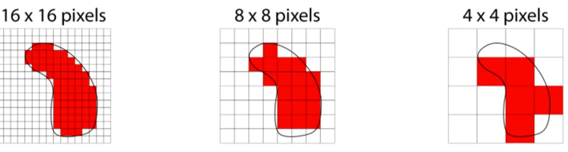
Figure 2.8: An illustration of resampling of images using the nearest neighbor assign-ment. Given the input image from a VHS image (left), the pixels are downsampled to a lower scale regarding to the nearest neighbor until it achieve the same size of multi/hyper spectral image (middle). Afterwards, the is applied an upsampled process to return to the original size image.
In this work, we use the nearest neighbor assignment to map the regions extracted from a VHS image to a set of pixels signatures in HS image, an example of mapping regions is showed in Fig 2.9. We also use the upsample nearest neighbor assignment method to analyze thematic maps created only using the spectral features, in the same size of the spatial domain.
18 Chapter 2. Related Work and Background
2.4
Supervised Learning
Supervised learning in computer vision, particularly in machine learning, is the problem of predict to which of a set of categories (or labels) a new observation belongs, on the basis of a training set of data, which contains observations (or instances) whose category is known. When the categories of the instances in the problem are discrete, the problem is named as classification.
In other words, a supervised learning algorithm analyzes the labeled training set of data, and creates a function, which is used to predict label of unseen observations. In an optimal scenario, the created function predicts correctly all the labels of the unseen instances.
There is an extensive range of supervised learning algorithms for the task of classification, each one with its own advantages and limitations, for that reason there is no best algorithm for all supervised learning problems.
A short explanation of well known supervised learning algorithms used in this work is showed below:
• Gaussian Naive Bayes: Naive Bayes methods are a set of supervised learning algorithms based on Bayes’ theorem and the naive assumption of independence between every pair of features. So, let the feature vector X = {x1, ..., xn} with
label y, the Bayes’ theorem assert:
P(y|x1, ..., xn) =
P(y)P(x1, ..., xn|y)
P(x1, ..., xn)
(2.1)
The independence assumption between the features lets us state:
∀xi :P(xi|y, x1, ..., xi−1, xi+1, ..., xn) =P(xi|y) (2.2)
So Equation 2.1 can be simplified to:
P(y|x1, ..., xn) =
P(y)Qn
i=1P(xi|y)
P(x1, ..., xn)
(2.3)
Since the factor P(x1, ..., xn) is constant for a given input, the following decision
function can be used as classification rule:
P(y|x1, ..., xn)∝P(y)
n
Y
i=1
2.4. Supervised Learning 19
y′ =argmax
y P(y) n
Y
i=1
P(xi|y) (2.5)
The different naive Bayes classifiers differ mainly by the assumptions they make regarding the distribution of P(xi|y). A Gaussian Naive Bayes algorithm uses
the estimation of P(xi|y) in concern with the Gaussian distribution:
P(xi|y) =
1
p
2πσ2
y
exp
−(xi−µy)
2
2σ2
y
(2.6)
• Support Vector Machines: The support vector machine is a supervised algo-rithm in machine learning, and it is often applied to the task of classification in the field of remote sensing.
The algorithm consists in the construction of a plane or a set of hyper-planes which is the farthest away from the closest training samples. The distance between the hyperplane and the closest training points is called the margin, which is the quantity maximized by the SVM. The SVM has as premise that a good separation of the observation samples at the feature space is achieved by using the hyper-plane that has the maximum margin value.
Consider a case which is linearly separable, and let a set ofnlabeled samplesX =
{x1, ..., xn} with labels Y = {y1, ..., yn} ∈ {−1,+1}. The SVM searches for the
hyper-plane given by the function F(x) =< w, x >+b maximizing the margin. It is proved in Boser et al. [1992], that maximizing the margin is equivalent to minimize the norm in the expression 1
2||w||2 under the restriction of yi(< w, x >
+b)≥1. So the SVM dual problem can be expressed as:
max
αi
( n X
i=1
αi −
1 2
n
X
i,j=1
αiαjyiyjhxi, xji
)
(2.7)
And the solution of the maximization above is expressed as:
hw, xi=
n
X
j=1
yjαjhxi, xji (2.8)
Where the points lying on the margin (also called support vectors) are the samples with Karush-Kuhn-Tucker multipliers αi equal to zero.
20 Chapter 2. Related Work and Background
is called the kernel trick, implicitly mapping their inputs into high-dimensional feature space.
• K-nearest neighbors: The K-nearest neighbors algorithm is one of most simple learning methods for classification task. The prediction of a new observation is given by the majority vote of the labels from the K-nearest neighbor samples at the training set. The performance of the algorithm depends of the two main factors: the parameter K of neighbors and the metric of distance between the samples. Since the algorithm is simple, it suffers in some cases: from data noise lets the algorithm insert outliers in the voting, high dimensional features let the computation of the distances meaningless ,unbalanced data let the most frequent class dominate a new prediction, etc.
• Decision Tree: The Decision Tree is a non-parametric method which aims to create a model that predicts the value of a target variable by learning simple de-cision rules inferred from the data features. To make this, the algorithm breaks down a dataset into smaller and smaller subsets while at the same time an associ-ated decision tree, which contains instances with similar values, is incrementally developed. The final result is a tree with decision nodes and leaf nodes, where the decision nodes are composed by two or more branches that separate sam-ples based on some measure (e.g., entropy, information gain), and the leaf nodes which assigned the final predict in concern to the path of decision nodes. Like the other algorithms, decision tree also has advantages and disadvantages. Some advantages of decision trees are: it is simple to understand and to interpret; it can handle numerical and categorical data; its prediction cost is logarithmic in the number of training data; etc. The disadvantages include: optimal decision tree is known to be NP-complete; it does not fit well with unbalanced data; it can be unstable in some small variations, etc.
• Adaboost: To explain the Adaboost method, we need to define the concepts of weak and strong learner:
Definition 5. A weak learner is defined as a classifier which is only slightly correlated with the true classification (it can label examples better than random guessing). In contrast, a strong learner is a classifier that is arbitrarily well-correlated with the true classification.
2.4. Supervised Learning 21
them and create a final strong learner. An example of the Adaboost learning is showed in Figure 3.2
Initial uniform weight on training data
weak classifier 1
Incorrect classifications re-weight more heavily
Final classifier is weighted combination of weak classifiers
weak classifier 2
weak classifier 3
H(x) = sign (α1h1(X) + α2h2(x) + α3h3(x))
Figure 2.10: An illustration of Adaboost iterations.
The data modifications at each so-called boosting iteration consist of applying weights w1, w2, ..., wN to each of the training samples. Initially, those weights
are all set to wi = 1/N-, so that the first step simply trains a weak learner on
the original data. For each successive iteration, the sample weights are individ-ually modified and the learning algorithm is reapplied to the reweighted data. At a given step, those training examples that were incorrectly predicted by the boosted model induced at the previous step have their weights increased, whereas the weights are decreased for those that were predicted correctly. As iterations proceed, examples that are difficult to predict receive ever-increasing influence. Each subsequent weak learner is thereby forced to concentrate on the examples that are missed by the previous ones in the sequence Hastie et al. [2001].
22 Chapter 2. Related Work and Background
Such as in computer vision, the concept of combining classifiers to improve the performance of individual classifiers is also explored in remote sensing. In [Du et al., 2012], the authors presented a review of the multiple classifier system (MCS) for RSI classification, and showed that a MSC can effectively improve the accuracy and sta-bility of classification, and diversity measures are important at decision in ensemble of multiple classifiers.
The most common techniques which involve the ensemble of classifiers are: Bag-ging [Breiman, 1996] and Boosting [Freund et al., 1996]. BagBag-ging uses bootstrap sam-pling to generate accurate ensemble Bagging [Breiman, 1996]. Boosting is a general method of producing a very accurate prediction rule by combining rough and mod-erately inaccurate learner [Freund et al., 1996]. Both techniques are extensively used in literature: [Du et al., 2015] proposed an improved random forest approach, which creates a voting-distribution ranked rule for handling with imbalanced samples for semantic classification of urban buildings combining VHR image and GIS data; [Woo and Do, 2015] presents a post-classification approach for change detection by using Ad-aBoost classifier; in [Boukir et al., 2015], the authors proposed a texture-based forest cover classification using random forests and ensemble margin in a very high resolution context.
Other methods for ensemble of classifiers are also exploited in remote sensing, such as neural networks in [Han and Liu, 2015], where the authors explored a combina-tion of a descriptor Non-negative Matrix Factorizacombina-tion (NMF) with Extreme Learning Machine (ELM) network as a base classifier of ensemble, comparing with bagging and adaboost algorithms for high resolution RSI classification.
2.5
Data Fusion
In data fusion, each data source describing the same scene and objects of interest can be defined as amodality.
In remote sensing image analysis, the different modalities often represent a par-ticular data property carrying complementary information about the surface observed [Farah et al., 2008].
2.5. Data Fusion 23
and almost insensitive to cloud cover, with difficult visual interpretation), showed in Figure 2.11.
Synthetic Aperture Radar (SAR) Optical Remote Sensing
Figure 2.11: On the left, the active SAR sensor almost insensitive to cloud cover; On the right, the passive optical sensor occlusion by cloud cover.
The joint complementarity exploitation of different remote sensing sources has proven to be very useful in many applications of land-cover classification, and the capability of improve the discrimination between the classes is a key aspect towards a detailed characterization of the earth [Dalla Mura et al., 2014], [Alonzo et al., 2014].
Concerning multisource data, a diversity of fusion techniques has been proposed in the remote sensing literature, which can be divided in levels according to the modalities used in the fusion, as follows:
1. Fusion at subpixel level: Given k modalities datasets, which usually involve different spatial scales, the modalities are fused at subpixel level using appropriate transforms [Delalieux et al., 2014]. These fusions are commonly used in the cases where the main objective is to preserve the valuable spectral information from multispectral or hyperspectral sensors, with low spatial resolution, as alternative of pansharpening methods which can produce a spectral distortion [Huang et al., 2014].
24 Chapter 2. Related Work and Background
measures; secondly, when distinct materials are combined into a homogeneous mixture (e.g., rocks on the soil).
The first reason arise in remote sensing platforms flying at a high altitude or per-forming wide-area surveillance, where low spatial resolution is common, however the second reason can occur independent of the spatial resolution of the sensor [Keshava and Mustard, 2002]. An illustration is showed in Figure 2.12.
Figure 2.12: Even for optical sensors, the mixture of pixels happens, and various materials can occupy a single pixel mutually.
The spectral unmixing is a procedure to identify, given a mixed pixel, the col-lection of constituent spectra, or endmembers, which corresponds to well known objects in the scene, and a set of corresponding fractions, or abundances, that indicate the proportion of each endmember present in the pixel. This allows the decomposition of each observed spectral signature into its constituent pure com-ponents, and provides subpixel resolution [[Keshava and Mustard, 2002], [Heylen et al., 2014]].
2.5. Data Fusion 25
An overview of the majority of nonlinear unmixing methods used in hyperspectral image processing, and many recent developments in remote sensing are presented with details in [[Heylen et al., 2014], [Lanaras et al., 2015]].
2. Fusion at pixel level: Given k modalities datasets, in the fusion at pixel level exists a direct pixel correlation between the modalities, which is used to produce data fusion.
In general, that fusion level attempts to combine data from different sources in intent to produce a new modality, which, afterwards, could be used for different applications. Some examples that rely on that case is pansharpening, super resolution and 3D reconstruction from 2D views [Dalla Mura et al., 2014]. An evaluation of spatial and spectral effectiveness of more common pixel-level fusion methods was realized in [Marcello et al., 2013]. Regarding [Marcello et al., 2013] several pan sharpening methods have been proposed in the literature [Zhang [2010], Amro et al. [2011], Stathaki [2011], Hong and Zhang [2008]], primarily based on algebraic operations, component substitution, high-pass filtering and multi resolution analysis.
A brief description of the most common and effective methods follows:
The Brovey Transform (Brovey) is one of the most simple fusion methods, which injects the overall brightness of the panchromatic image into each pixel of the normalized multi or hyper spectral bands regarding to an algebraic expression. The Synthetic Variable Ratio (SVR) and Ratio Enhancement (RE) are similar methods which use more interesting methods to normalize the spectral data.
The Intensity-Hue-Saturation (IHS) transformation extracts from the spec-tral RGB image the spatial (I) and specspec-tral (H,S) information, to afterwards replace the I component by the PAN image and doing the reverse IHS transform to inject the spatial information.
The PCA fusion method projects the original spectral bands in the principal components, and as assumption that the first principal component (high variance) has the major spatial information. Hence the first principal component is replaced by the PAN image and applied the inverse transformation to produce a combined information data.
26 Chapter 2. Related Work and Background
made using a pyramidal scheme established on convolutions followed by a decima-tion operadecima-tion. At the end, the invert transform is made using the multi spectral approximation image and the PAN wavelet coefficients [Cao et al., 2006].
The À trous (Atrous) fusion method is based on the undecimated dyadic wavelet transform (a shift invariant of discrete wavelet transform). The original image is decomposed into approximation images and a sequence of new image called wavelet planes. The wavelet planes keep the detail information and are computed as the differences between two consecutive approximations. The fused images are obtained, adding the wavelet planes to the MS approximation [Chen et al., 2008].
The standard fusion algorithms mentioned above (IHS, BT and PCA) have been widely used for relatively simple and time efficient fusion schemes, but they have inherent problems such as: these pixel-level fusion methods are sensitive to regis-tration accuracy, so that co-regisregis-tration of modalities images at sub-pixel level is required for a good result; Brovey and IHS transforms have a limitation of three or less spectral bands; and even improving the spatial resolution they tend to distort the original spectral signatures.
More recently, [Gharbia et al., 2014] made an analysis of the fusion techniques in image (IHS, BT and PCA) also applied to remote sensing at pixel level, showing that all techniques have their own limitation when used individually and they also encouraged the utilization of hybrid systems.
3. Fusion at feature level: Given k modalities datasets, various features are extracted individually from each modality, e.g., edges, corners, lines, texture parameters, followed by a fusion, which involves extraction and selection of more discriminant attributes.
2.5. Data Fusion 27
(a) High-resolution panchromatic image (b) Lower resolution multispectral image
(c) Single high-resolution color image
Figure 2.13: An illustration of a Pansharpening process. Given a panchromatic high spatial resolution image (a) and a multispectral low spatial resolution image (b), an out-put is created by using a Pansharpening technique resulting in a single high-resolution color image.
For example, in the context of classification with Lidar and optical image, to handle both sources as input to a classifier, the registration problems should be solved (e.g., by rasterizing the Lidar data to the same spatial resolution of the optical image).
Regarding [Gomez-Chova et al., 2015], one of the new research directions on feature level multimodal fusion are the Kernel methods. At the domain of remote sensing, there is a considerable number of studies about kernel methods [Camps-Valls and Bruzzone, 2009], once they provide a instinctive way to encode data from different modalities into classification and prediction models.
The advantages to use the kernel function are the mathematical properties, such as: the sum of two valid kernels and a product of a kernel by a positive scalar stills a valid kernel function. Therefore, kernels of different data modalities can be easily combined, thus providing a multimodal data representation.
28 Chapter 2. Related Work and Background
combination of kernel functions, was realized by Camps-Valls et al. [2006], who created a compound kernel by using the weighted summation of spatial and spec-tral features from the co-registered region.
Extending the proposition for more than two sources, a multiple kernel learning [Rakotomamonjy et al., 2008] was applied to Tuia et al. [2010b] for combining spatial and spectral information, to combine optical and radar data [Camps-Valls et al., 2008], [Tuia et al., 2010a], using the same sensor but in different places [Gómez-Chova et al., 2010], also using different optical sensors to change detection [Volpi et al., 2015]. In all these examples, a kernel matrix was created for every data source and then use a linear combination to create a more reliable multimodal similarity matrix.
4. Fusion at decision level: Given k modalities datasets, an individual process path is made for each modality, followed by a fusion of the outputs, assuming that the k outputs combined can improve the final accuracy [Li et al., 2014].
In this way, the combination of complementary information from different modal-ities is done through the fusion of the results obtained considering each modality independently.
The method relies on the fact of the individual predictions that are in agreement are confirmed due to their consensus, whereas the decisions that are in discor-dance are combined (e.g., via majority voting) in the attempt of decreasing the errors, expecting to increase the robustness of the decision.
There are several ways to combine the decisions, such as including voting meth-ods, statistical methmeth-ods, fuzzy logic-based methmeth-ods, etc. When the results are explained as confidences instead than decision, the methods are called soft fusion; otherwise they are called hard fusion.
An example of this type of fusion was presented in the 2008 [Licciardi et al., 2009] and 2009-10 [Longbotham et al., 2012] data fusion contests. Wang et al. [2015] used a scheme of weighted decision fusion, which uses the SVM and the Random Forest for the probability estimation in the Landsat 8 and MODIS sensors; Liao et al. [2014] made a combination of fusion by feature level using a graph-based feature fusion method together with a weight majority voting of outputs from differents SVM’s to the classification of hyperspectral and LiDAR data.
2.5. Data Fusion 29
Chapter 3
Methodology
We propose two different approaches to deal with classification task exploiting data from multiple sensors:
1. Dynamic Majority Vote: A late fusion technique that exploits the specialty of different classifiers and combines them for a final decision for each pixel in the thematic map. This approach was designed to handle only multi class problems.
2. Boosting Approach: A combination of three levels of fusion: pixel, feature and decision level; which exploits different types of features, extracted from various sensors using a boosting based approach. Differently of the Dynamic Majority Vote, this method can handle binary and multi class problems.
In this chapter, we describe the proposed approaches, Dynamic Majority Vote in Section 3.1, and Boosting Approach in Section 3.2. Figure 3.1 illustrates a base framework used in both strategies proposed.
Before describing our proposed approaches, let us first define some of the notations that will be used throughout this dissertation in Table 3.1.
3.1
Dynamic Majority Vote
The proposed method aims at exploiting multi-sensor data in a more general way, instead of project to deal with a specific scenario or a particular region. We create a framework based on a supervised learning scheme, dealing with different scenarios, regions and objects, on the creation of thematic maps for the classification task. For that, we propose a new approach, at decision level, to handle an amount of decisions from different classifiers, and combine them to obtain a final decision for each pixel in
32 Chapter 3. Methodology
Object Representation
Feature Extraction
Hyper Spatial Image Hyperspectral Image
Classification
Segmentation Pixel Spectral Signature
Data Input
Region Based Features Dimensionality Reduction
v1 v2
v4 v3
Classifiers
F(x)
(1)
(2)
(3)
(4)
Figure 3.1: An illustration of the base framework used in both strategies proposed. (1) The proposed method is projected to receive two images from the same place with different domains as input: an image with very high spatial resolution and another one with hyperspectral resolution; (2) the VHS image is segmented in regions using a segmentation algorithm while the HS image is analyzed by the spectral signature of each pixel; (3) feature vectors are extracted from the segmented regions of VHS using various descriptors and the spectral signatures are projected by using different dimensionality reduction methods; (4) using different learning methods and the feature vectors extracted from both domains is created a collection of base classifiers, which together are combined to create a strong classifier F(X).
3.1. Dynamic Majority Vote 33
Table 3.1: Notations
IV HS Image at the VHS resolution domain
IHS Image at the HS resolution domain
Yt
R Image labels of the training data
Yt′
R Image labels of the test data
YR=YRt∪Yt
′
R Image labels of the entire data
Wdyn Dynamic Weight Matrix
C ={ci ∈C,1< i≤ |C|, i∈N∗}
A set of trained classifiers ci over
different features from spatial and spectral domains.
MC ={Mj ∈MC,1< j ≤ |C|, j ∈N∗}
A set of confusion matrices Mj
computed fromcj at the validation
setYv R.
L={lk ∈L,2< k ≤ |L|, k∈N∗} A set of all classes |L| in the problem.
the thematic map. Contrary to approaches from the literature, our method uses the kappa index [Congalton and Green, 2008] to compare two classifiers. This fact brings some advantages since kappa index is more robust in dealing with unbalanced training sets, as showed in Section 4.2.
The proposed method is projected to receive two images from the same place with different domains as input: an image with very high spatial (V HS) resolution and another one with hyperspectral (HS) resolution. Our method is developed for a multiclass mapping scenario. It exploits the expertise of each learning approach over each class in order to find the most specialized classifiers. The result of this process is a dynamic weight matrix.
Most voting methods use an unique weight assigned to each classifier, regardless of the class to be predicted. This approach does not exploit the specialty of each classifier in a particular class, and thus can weaken the final model with no reliable predictions. Another weakness of the traditional majority voting is the difficulty of dealing with classifiers that produce similar mistakes in their predictions, thus resulting in the prediction of incorrect class.
The proposed approach uses a method for assigning weights where each classifier has a degree of reliability for each class to be predicted, resulting in dynamic weights. In addition, the method was created to handle classifiers that produce similar mistakes in their predictions. For this, an update of weights is accomplished favoring models whose distribution errors is uniform, thus hindering the allocation of high weight for classifiers not experts in difficult samples.
ex-34 Chapter 3. Methodology
traction, training, dynamic weight matrix construction, and predicting. Figure 3.2 illustrates the proposed framework. We detail each step next.
Object Representation
Feature Extraction
Hyper Spatial Image Hyperspectral Image
Classification
Segmentation Pixel Spectral Signature
Data Input
Region Based Features Dimensionality Reduction
v1 v2
v4 v3
TP FN
FP TN
Confusion Matrices
w1,1 w1,2 w1,l-1 w1,l w2,1 w2,2 w2,l-1 w2,l
wc,1 wc,2 wc,l-1 wc,l Classifiers
Classes
Dynamic Weight Matrix
Matrices Analysis Dynamic Weight Matrix
Construction Validation Data Base Classifiers Prediction (3) (2) (1)
3.1. Dynamic Majority Vote 35
3.1.1
Object Representation
The first step is to delineate the objects to be described by the feature extraction algorithms. For the IV HS image, we perform a segmentation process over the regions
of Yt
R in order to split the entire image into more spatially homogeneous objects. It
allows the codification of suitable texture features for each part of the image.
Due to the low spatial resolution of the IHS image, we consider the pixel as the
unique spatial unit. Anyway, we are more interested in exploiting the spectral signature of each pixel.
For more details about the object representation phase forIVHSandIHS, please
refer to Chapter 2.
3.1.2
Feature Extraction
Concerning IV HS image, we have used image descriptors based on visible color and
texture information to encode complementary features. For the IHS image, we exploit
dimensionality reduction/projection properties from the spectral signature in order to obtain diversity.
3.1.3
Training
Let Yv
R ⊂ YRt be a validation set separated from the training set. We use the features
extracted by each descriptor over the remaining training samples and a set of learn-ing methods to create an amount of classifiers (tuples of descriptor/learnlearn-ing method). We use the obtained classifiers to learn the probability distribution of the training set. Notice, that training process requires a region mapping between spatial and spec-tral resolutions, using an interpolation method, since IV HS and IHS images are from
different domains.
3.1.4
Dynamic Weight Matrix Construction
Algorithm 1 outlines the proposed steps for the construction of the dynamic weight matrix (Wdyn).
In initializing phase, we create the Wdyn ∈ R|L|x|C| with all values set to zero.
Afterwards we compute for every Mi the Cohen’s kappa value (κci) along with the
mean kappa value (κmean), which will help the model to reject the base classifiers with
high disagreement in comparison to the average (Lines 1-2). The Wdyn is built in a top
36 Chapter 3. Methodology
Algorithm 1 Construction of the Dynamic Weight Matrix.
1 Input: Stack of Confusion Matrices (MC) 2 Initializing: Set Wdyn ← 0, individual κc
i and mean ¯κ kappa index.
3 for each class lk inL do
4 Creating of a sorted list of pairs (hl
k|ci)
5 for every pair(hl
k/ci) at position j do
6 Initial weight in Wdyn ←(j)/|C| 7 Compute the sparsity SM
i ← maxmiss/(hits+misses)
8 Compute mexp ← pmiss/(|L| −1)
9 if κc
i >κ¯ then
10 if SM
i <2∗mexp then
11 Gain atWdyn ← (κc
i/¯κ)*Wdyn
12 else
13 Penalty atWdyn ← (¯κ/κc
i)*Wdyn
14 end for 15 end for
row) until the last classl|L|(last row). Therefore, for each classlk, the hits at the class
lk (hlk) are extracted from MC, and a list of pairs (hlk|ci) sorted by the hlk is created
(Lines 3-4). For every pair(hlk|ci), an initial weight is assigned inWdyn, regarding with
the positionj of the pair (hlk|ci)in the sorted list, thus the lowest element (j = 1) will
receive 1
|C| and the higher element (j = |C|) receive
j
|C| = 1 (Line 5-6). In Lines 7-8,
the columnk in respect of lk from each Mi ∈MC is used to compute two coefficients,
named as:
1. The sparsity SMi, which indicates the degree of importance of ci at lk, given
by the ratio of the highest miss value at column k (maxmiss) and the sum of all
predicts (hits and misses); A higher value of SMi means a higher confusion of the
predictions from Mi to the classlk.
2. The uniform misses expected for each class (mexp), given by the miss rate
(pmiss) uniformly distributed to the other classes. As named, this coefficient
measure the explained percentage of misses expected for each class if ci error
were equally distribute for all classes.
Finally, at Lines 9-13 the weights of Wdyn are updated when the kappa index of
ci (κci) is greater than the mean of all classifiers kappa’s index (κ¯). When SMi is less
than twice times the mexp, the weight in Wdyn for ci in lk is increased and decreased
otherwise, regarding with the ratio between κci and κ¯. The reweight in the Wdyn aims
3.1. Dynamic Majority Vote 37
those classifiers which show a sparsity (or density) in the predicts by class, at the confusion matrix, regarding to the validation set.
An illustration of the Wdyn construction is showed in the Figure 3.3.
M1 M1 M2 M2 M3 M3 Sort
κM1 κM2 κM3 κmean = (κM1+κM2+κM3)/3
DWM Initial weight
7
7 2 1
3 5 3 7 3 3 5 5 1 1 12 12 2 2 1 1 2 2 0 0 1 1 3 3 3 3 2 7 4 3 4 2 1 2 1 3 0 6 2 2 0 9 3 8 4 1 0 3 0 3 5 1 1 8 3 0 1 1 1 1 1 2 Predicted True Label
M1 M2 M3
Predicted Predicted
True Label True Label
1 3
SM1 = 3/10 mexp = (5/10 * 1/3)
SM2 = 1/10 mexp = (3/10 * 1/3)
SM3 = 12/20 mexp = (17/20 * 1/3)
30% < 33% SM1 < 2*mexp
DWM(M1,class 1) =
10% < 20% SM2 < 2*mexp
DWM(M2,class 1) =
60% > 56% SM3 < 2*mexp
DWM(M3,class 1) = 2 3
κM1 κmean *
1 κM2
κmean * 1 3 κmean κM3 * Gain Weight Penalty Weight Gain Weight
Sparsity Miss expected
(1)
(2)
(3)
(4)
(5)
Figure 3.3: An example of the construction of Dynamic Weight Matrix (DWM), re-garding to the class 1. The process starts in (1) by receiving the confusion matrices of the base classifiers and selecting the number of correct samples in the class 1 from each matrix. Then, in (2) an array of correct predictions is sorted and an initial weight is assigned to the DWM first line, regarding to the previous sorted array. Afterwards, the measures of Sparsity and Miss Expected are computed in (3), analyzing the dispersion of the uncorrected samples labeled to class 1. Thereafter, the kappa metric value of each matrix is computed in (4), followed by the mean kappa value. After that, the initial weights of DWM are updated in (5) when the kappa index of a matrix is greater than the mean kappa value previously computed.
3.1.5
Predicting
Once the Wdyn is built, the same method of segmentation is used in Yt
′
R, and the
seg-mented objects are labeled by the classifiers as regions (spatial tuple) or pixel by pixel (spectral tuple) creating a thematic map for each classifier. Once more, since the the-matic maps from theIHS image have a different resolution, we apply the same upsample
38 Chapter 3. Methodology
and taking the final decision according to the highest final weight class for that pixel in specific. An example of how to use theWdyn is showed in Figure 3.4.
Figure 3.4: Given the output of the classifiers in a pixel, the relevance of each prediction is given by the dynamic weight matrix, afterwards these relevances are added regarding to the output of each classifier and the class with the highest final weight is chosen.
3.2
Boosting-Based Approach
The proposed method aims at exploiting multi-sensor data in a more general way, using the idea of boosting of classifiers, based on the SAMME Adaboost [Zhu et al., 2009].
3.2. Boosting-Based Approach 39
We create a framework based on a supervised learning scheme, dealing with different scenarios, regions and objects, on the creation of thematic maps for the clas-sification task. We propose a scheme, with a combination of pixel, feature and decision levels, to handle an amount of information from different modalities, and combine them for a final decision for each pixel in the thematic map. Contrary to approaches from the literature, our method uses the inherent feature selection of the Adaboost for the combination of different modalities, as a natural process.
The proposed method is projected to receive two images from the same place with different domains as input: an image with very high spatial resolution and another one with hyperspectral resolution.
The boosting approach is divided into four main steps: object representation, feature extraction, training, predicting. Figure 3.5 illustrates the proposed framework. We detail each step next.
3.2.1
Object Representation
The first step is to define the objects to be described by the feature extraction algo-rithms. For theIV HS image, we perform a segmentation process over the regions ofYRt
in order to split the entire image into more spatially homogeneous objects. It allows the codification of suitable texture features for each part of the image.
Due to the low spatial resolution of the IHS image, we consider the pixel as the
unique spatial unit. Anyway, we are more interested in exploiting the spectral signature of each pixel.
For more details about the object representation phase forIVHSandIHS, please
refer to Chapter 2.
3.2.2
Feature Extraction
Concerning IV HS image, we have used image descriptors based on visible color and
texture information to encode complementary features. For the IHS image, we exploit
dimensionality reduction/projection properties from the spectral signature in order to obtain diversity. Notice that feature extraction process requires a region mapping between spatial and spectral resolutions, since IV HS and IHS images are from different