Adv. Sci. Res., 12, 207–218, 2015 www.adv-sci-res.net/12/207/2015/ doi:10.5194/asr-12-207-2015
© Author(s) 2015. CC Attribution 3.0 License.
EMS
Ann
ual
Meeting
&
10th
European
Conf
erence
on
Applied
Climatology
(ECA
C)
Methodologies to characterize uncertainties in regional
reanalyses
M. Borsche1, A. K. Kaiser-Weiss1, P. Undén2, and F. Kaspar1
1Deutscher Wetterdienst, National Climate Monitoring, Frankfurter Str. 135, 63067 Offenbach, Germany 2Swedish Meteorological and Hydrological Institute, Folkborgsvägen 17, 601 76 Norrköping, Sweden
Correspondence to:M. Borsche ([email protected])
Received: 25 January 2015 – Revised: 2 October 2015 – Accepted: 16 October 2015 – Published: 27 October 2015
Abstract. When using climate data for various applications, users are confronted with the difficulty to assess the uncertainties of the data. For both in-situ and remote sensing data the issues of representativeness, homogene-ity, and coverage have to be considered for the past, and their respective change over time has to be considered for any interpretation of trends. A synthesis of observations can be obtained by employing data assimilation with numerical weather prediction (NWP) models resulting in a meteorological reanalysis. Global reanalyses can be used as boundary conditions for regional reanalyses (RRAs), which run in a limited area (Europe in our case) with higher spatial and temporal resolution, and allow for assimilation of more regionally representative observations. With the spatially highly resolved RRAs, which exhibit smaller scale information, a more realistic representation of extreme events (e.g. of precipitation) compared to global reanalyses is aimed for. In this study, we discuss different methods for quantifying the uncertainty of the RRAs to answer the question to which extent the smaller scale information (or resulting statistics) provided by the RRAs can be relied on. Within the European Union’s seventh Framework Programme (EU FP7) project Uncertainties in Ensembles of Regional Re-Analyses (UERRA) ensembles of RRAs (both multi-model and single model ensembles) are produced and their uncer-tainties are quantified. Here we explore the following methods for characterizing the unceruncer-tainties of the RRAs: (A) analyzing the feedback statistics of the assimilation systems, (B) validation against station measurements and (C) grids derived thereof, and (D) against gridded satellite data products. The RRA ensembles (E) provide the opportunity to derive ensemble scores like ensemble spread and other special probabilistic skill scores. Finally, user applications (F) are considered. The various methods are related to user questions they can help to answer.
1 Introduction
Atmospheric reanalyses produce complete and physically consistent data products aiming for a best estimate of the state of the Earth’s atmosphere (Dee et al., 2014). In the European Union’s seventh Framework Programme (EU FP7) project Uncertainties in Ensembles of Regional Re-Analyses (UERRA), various European meteorological regional reanalyses (RRAs) are developed. Users turn to the spatially highly resolved RRAs for smaller scale information and a more realistic representation of extreme events (e.g. of precipitation) compared to global reanalyses, and would like to derive trends.
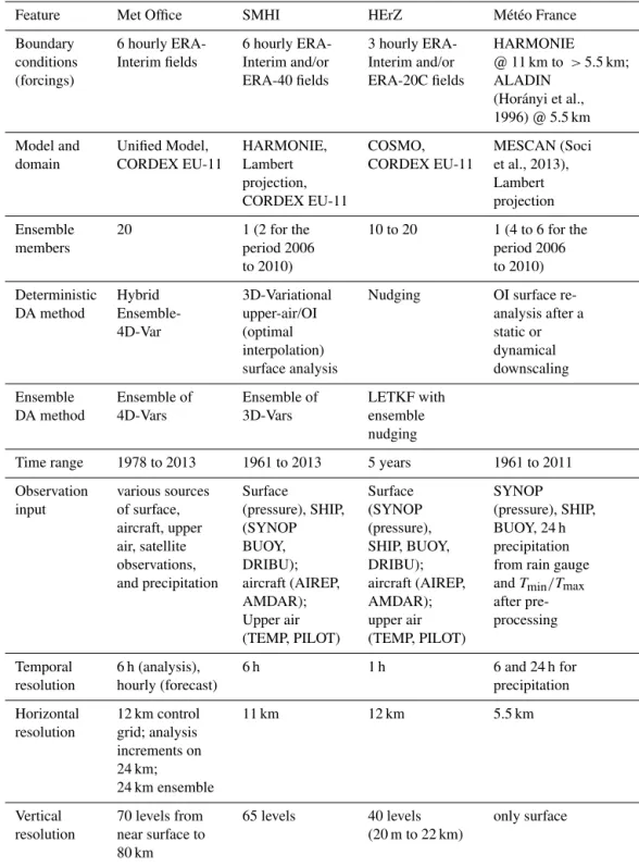
Table 1.Description of the regional reanalysis planned in the UERRA project.
Feature Met Office SMHI HErZ Météo France Boundary 6 hourly ERA- 6 hourly ERA- 3 hourly ERA- HARMONIE conditions Interim fields Interim and/or Interim and/or @ 11 km to >5.5 km; (forcings) ERA-40 fields ERA-20C fields ALADIN
(Horányi et al., 1996) @ 5.5 km Model and Unified Model, HARMONIE, COSMO, MESCAN (Soci domain CORDEX EU-11 Lambert CORDEX EU-11 et al., 2013),
projection, Lambert CORDEX EU-11 projection Ensemble 20 1 (2 for the 10 to 20 1 (4 to 6 for the members period 2006 period 2006
to 2010) to 2010) Deterministic Hybrid 3D-Variational Nudging OI surface re-DA method Ensemble- upper-air/OI analysis after a
4D-Var (optimal static or interpolation) dynamical surface analysis downscaling Ensemble Ensemble of Ensemble of LETKF with
DA method 4D-Vars 3D-Vars ensemble nudging
Time range 1978 to 2013 1961 to 2013 5 years 1961 to 2011 Observation various sources Surface Surface SYNOP input of surface, (pressure), SHIP, (SYNOP (pressure), SHIP,
aircraft, upper (SYNOP (pressure), BUOY, 24 h air, satellite BUOY, SHIP, BUOY, precipitation observations, DRIBU); DRIBU); from rain gauge and precipitation aircraft (AIREP, aircraft (AIREP, andTmin/Tmax
AMDAR); AMDAR); after pre-Upper air upper air processing (TEMP, PILOT) (TEMP, PILOT)
Temporal 6 h (analysis), 6 h 1 h 6 and 24 h for resolution hourly (forecast) precipitation Horizontal 12 km control 11 km 12 km 5.5 km resolution grid; analysis
increments on 24 km; 24 km ensemble
Vertical 70 levels from 65 levels 40 levels only surface resolution near surface to (20 m to 22 km)
80 km
Table 1 summarizes the RRAs which are planned to be produced within the UERRA project at the Met Office (MO), Exeter, UK (developed upon Renshaw, 2013); the Swedish Meteorological and Hydrological Institute (SMHI), Nor-rköping, Sweden (developed upon Dahlgren et al., 2014 and now Bubnova et al., 1995); DWD’s (Deutscher Wetterdi-enst) Hans-Ertel Centre for Weather Research (HErZ; Sim-mer et al., 2015) University of Bonn, Germany (Bollmeyer
reanalysis whereas for the ensemble realizations it is planned to take lateral boundary conditions from ERA-20C (Poli et al., 2013) or ERA5, the successor of ERA-Interim, into ac-count.
These three groups (MO, SMHI, HErZ) develop RRAs based on their operational NWP models, which are the Uni-fied Model (Davies et al., 2006), the HARMONIE model (Bubnova et al., 1995; De Troch et al., 2013; Gerard et al., 2009), and the COnsortium for Small-scale MOdelling (COSMO) model (Schättler et al., 2014), respectively. They plan to produce a deterministic run and a set of ensembles of reanalyses with up to 20 members each. The data assimila-tion methods employed by MO are a hybrid 4DVar (Clayton et al., 2013) for the deterministic run and an ensemble of 4D-Vars (Rawlins et al., 2007) for the ensemble runs. SMHI has implemented a 3D-Var (Berre, 2000; Fischer et al., 2005) for the deterministic run and an ensemble of (2) 3D-Vars (using the ALADIN and ALARO-0 physics versions as de-scribed in De Troch et al., 2013) for the ensemble runs. HErZ uses nudging and is developing a Local Ensemble Trans-form Kalman Filter (LETKF) (Hunt et al., 2007; Harnisch and Keil, 2015) with Ensemble Nudging for the determinis-tic and ensemble runs, respectively. Ensembles are created either by perturbed initial conditions (MO), disturbed model physics (SMHI), disturbed observations (HErZ), or a com-bination of these. Météo-France performs an additional sta-tistical and dynamical downscaling of the RRAs produced at SMHI followed by high resolution reanalysis for the surface only in order to drive inter alias hydrological physical mod-els. The data sets are planned to span several decades, and a few years for the more experimental set-ups. SMHI produces in addition a cloudiness reanalysis (based on Häggmark et al., 2000) using a consistent satellite data set.
An estimation of uncertainty is required by users on dif-ferent temporal and spatial scales for enabling and enhancing applications of RRA products. Section 2 outlines the meth-ods, relying on assimilation feedback, comparison against station observations, gridded station observations, gridded satellite remote sensing based data products, and ensembles. We also discuss deriving uncertainty estimation from user applications. The advantages and disadvantages of the var-ious methods are discussed and they are related to varvar-ious scientific and user questions. The meteorological parameters for which each method is feasible depend mainly on prac-tical considerations. In Sect. 3, the various skill scores are summarized, the suitability of which depends on the meteo-rological parameters and the question sought to be answered. In Sect. 4, a summary and recommendations for best prac-tises are given.
2 Methods to estimate uncertainties in RRAs
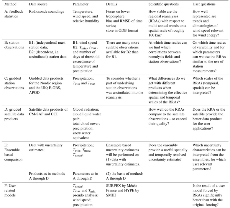
Table 2 summarizes six methods which have been discussed within the UERRA project and correspond to those discussed
in the EU FP7 project Coordinating Earth Observation Data Validation for Re-analysis for Climate Services (CORE-CLIMAX), see Kaiser-Weiss et al. (2015). Each of the meth-ods is discussed in this section, benefits and drawbacks pointed out, and the principle aim pursued with each method condensed into a scientific and a user question. Furthermore, the discussion below addresses both random and systematic uncertainties. A systematic uncertainty (which can depend on time as well as location or meteorological situation) is referred to as bias. Random uncertainties are characterized with the root mean square (RMS) against some data set con-sidered as truth, in case of absence of error estimates of the latter.
2.1 Method A: feedback statistics
Here, we distinguish between virtually independent observa-tions (not assimilated yet) and dependent observaobserva-tions (ob-servations passed through the assimilation system prior to the production of the reanalysis field). Strictly speaking, any observation system biased relative to the model will yield the analysis biased, and in this sense, measurements at later points in time are not strictly independent (as they are subject to this bias, too). Strictly independent data are hard to come by, especially for longer time periods, because they would naturally be selected for assimilation. Integrated parameters, such as precipitation, are strictly independent for most re-analysis systems. Further, minimum and maximum tempera-tures are not assimilated (though would not be strictly inde-pendent in case of biases). In order to maintain a reasonable large data base, we have to loosen our requirements on in-dependence such that we use virtually independent data as if they were strictly independent.
We regard the feedback as the output of the assimila-tion system in observaassimila-tion space. The feedback comprises the assimilated observations (bias corrected where applica-ble) (o), the background or “free forecast” (the short range forecast used in the data assimilation) (Hb), and the
analy-sis (Ha). The background and the analysis are brought into
observation space with the matrix of the linearized observa-tion operatorH, so a direct comparison between observations and model parameters can be performed in an optimal way. We check the feedback for trends and seasonal dependency (which are not desirable).
Usually, feedback statistics are a standard output of the data assimilation system and are frequently used by the pro-ducers for quality control. Note that, when comparing dif-ferent systems, the bias correction might differ. For one sys-tem, an approximately Gaussian distribution is expected for botho−Hbando−Ha, where the absolute value ofo−Hb
is the bias between observations and modelled observations, i.e. even if the difference is zero, both terms could be biased versus the (unknown) truth.
reanaly-Table 2.Methods and data sources suitable to derive uncertainty estimates for regional reanalyses.
Method Data source Parameter Details Scientific questions User questions
A: feedback Radiosonde soundings Temperature, Focus on lower How stable are the How well statistics wind speed, and troposphere; regional reanalyses represented are
relative humidity bias and RMSE of time (RRAs) with respect to trends and series; multi-annual trends on a climatologies of store in ODB format spatial scale of roughly wind speed relevant
100 km? for wind energy?
B: station B1: (independent) mast B1: wind speed There are many more At which time scales can On which time scales observations station data; B2:Tmin,Tmax, suitable observations we find which of variability and for
B2: (dependent, i.e. and number of available for B2 than correlations between which parameters assimilated) station data days of threshold for B1. reanalysis fields and can we use the RRAs
exceedance of station observations? similar to the use of
temperature and station
precipitation measurements?
C: gridded Gridded data products Precipitation; To consider whether a What differences do we Which scales of the station for the Nordic region TminandTmax part of underlying get with different RRAs (temporal,
observations and the UK; E-OBS, station observations products when spatial) can be APGD was assimilated into the determining the effective interpreted?
reanalysis. spatial and temporal scales of the RRAs?
D: gridded Satellite data products of Global radiation; How well do the RRAs Does the RRA or the satellite data CM-SAF and CCI cloud liquid water compare to the satellite satellite provide the
products path; observations – or exceed better data product
total cloud cover; their quality? for the user
precipitation; applications?
snow water equivalent
E: Data with uncertainty Precipitation; Ensemble based Does the ensemble Which uncertainty Ensemble estimates; Tmin,Tmax, uncertainty estimates provide a useful spatially characteristics can be
based Tmean; will be performed on and temporally resolved interpreted from the
comparison (1) data with uncertainty estimate? ensembles, for which
uncertainty estimates. user relevant parameters? Products as in methods Parameters as in (2) the basis of methods
A through D A through D A through D
F: User Tmean; SURFEX by Météo Is the result of a user
related TmaxandTmin France and HYPE by model forced by
models pseudo analysis; SMHI RRAs significantly
wind speed; better than with the
precipitation; original forcing?
sis systems, which do not differ much in their bias correction. Especially suitable for this purpose are radiosondes (temper-ature, wind speed and direction, and relative humidity). The core scientific interest in applying feedback statistics for val-idating the RRAs is how stable the RRAs are with respect to multi-annual trends on different spatial scales for these parameters. For instance, users of wind energy applications want to know how well represented the wind speed at heights relevant to wind energy is, especially with respect to trends and frequency distributions. Feedback statistics can of course be applied to all sorts of assimilated observations in order to perform the afore mentioned task. However, assimilated ra-diosonde data best fit the purpose of this method due to the
fact that they are used throughout the different RRA systems as anchor-data (i.e. no bias corrections applied). In contrast, aircraft data are handled specifically for each assimilation system (due to data thinning, data selection, and individual pre-processing) which renders inter-comparison of that data source much more difficult.
When, firstly, comparing the mean or RMS ofo−Hb
be-tween different reanalysis systems, it is crucial that compa-rable forecast lengths are selected. If this is valido−Hbis a
good measure to start with as a means of comparing against virtually independent observations. A smallero−Hb, i.e. a
per-spective, (2) the bias removal prior to the assimilation was successful – desired for the assimilation, (3) the background and the observations have the same bias against the truth – unlikely when a number of observing systems yield simi-lar results, (4) the model is biased due to the assimilation of biased observations in the previous step – also unlikely when a number of observing systems yield similar results. Secondly, in a successful assimilation, the average RMS of
o−Ha should be smaller than the average RMSo−Hbfor each observing system. Note that the mean or RMS ofo−Ha
is harder to compare between different reanalysis systems. Desroziers et al. (2005) provide a methodology of the di-agnosis in observation space and show that the variance of
o−Hbis the sum of the variance of background error in
ob-servation space (σ bf)2 and the variance of observation error (σ of)2, compare their Eq. (1):
1
N N X
i=1
oi−Hbi
oi−Hbi
!
= σ bf2+(σ of)2.
Further, they show that the background error covariance in observation space can be related to the product ofHa−Hb
ando−Hb, see their Eq. (2), and the observation error
co-variance can be related to the product ofo−Haando−Hb,
see their Eq. (3). Finally, if the error covariances are cor-rectly specified in the analyses, the product ofHa−Hband o−Ha should relate to the analysis-error covariance (see
their Eq. 4).
Before Desroziers et al. (2005), Hollingsworth and Lönnberg (1986) and Lönnberg and Hollingsworth (1986) applied a curve fitting of the covariances as a function of dis-tance to separated background errors from observation error based on the assumption that forecasts errors are horizon-tally homogeneous and observation errors are horizonhorizon-tally uncorrelated, where it is understood that the observation er-ror includes the representativeness erer-ror (also known as sam-pling error) as well as instrumental errors. This means a sep-aration of background bias and observation bias by inspec-tion of the spatial structure of mean background departures mean(o−Hb) for, e.g. each season or time of the day. It is
well known that the NWP models used in the data assimila-tion exhibit biases that have both diurnal and seasonal vari-ations. Thus, inspecting horizontal plots of biases at station locations (or possibly from a gridding interpolation proce-dure) will show if there is a significant background model bias. This is the case if there are spatially consistent mean departures that are sizeable compared with the RMS of the departures. In addition, this can be found by looking at the mean of the analysis increments mean(a−b) in grid point space.
On the other hand, if there are large variations of the mean background departures from station to station without hori-zontal consistency one may conclude that the bias is in the observation itself, or in some cases, due to poor representa-tiveness of the NPW model background at the specific
loca-tion. It may be due to occasional large departures between model orography and the one of the station or very different surface properties. The latter is expected to be the case only for a small portion of the stations and manual inspections of the data can reveal if it is the case. Either way, stations with large biases should be excluded for evaluations of random errors and used with special care when studying trends.
Multi-annual trends in the RRAs are determined by the boundary conditions (lateral boundary from the global re-analysis as well as the lower boundary, especially by the soil moisture and sea surface temperature), and the assimilated observations, where any trend in the observation system bias (relative to the model) would influence trends in the reanaly-sis. The latter might be expected to happen in regions where the observation coverage changed significantly over time.
The advantages of applying method (A) is that it provides a relative measure and can detect discontinuities and breaks as well as slowly increasing or decreasing systematic errors of the analyses (which all would influence trends). These re-sults are dependent on the weight the observations are given in the different data assimilation systems, thus they need to be inter-compared between the different RRAs with care. A drawback of this method is that inter-comparison between the feedback statistics of different reanalysis systems is in principle difficult mainly because the handling of the obser-vations may differ from one centre to another. For some of the parameters of interest (like, e.g. precipitation), the bias and RMSE are not sufficient scores to perform a thorough statistical analysis, thus more than these standard parameters should be evaluated based on the feedback. Note this method is limited in application to parameters which are assimilated.
2.2 Method B: station observations
Method (B) describes the comparison against point mea-surements from station observations. Interpreting single grid cells from the regional reanalysis and taking it as a proxy for a single point poses several questions from a theoreti-cal point of view, such as that of the representativeness of the NWP model for a given observation location and observ-ing method. However, the benefit of the method is that from a practical point of view this is often the easiest approach. Users of the RRAs are very much interested to answer the question how well the reanalyses compare against (their own) independent observation time series. This boils down to the question at what time scales correlations can be found be-tween RRA fields and station observations.
The major drawback of the method is that a point measure-ment cannot be expected to closely match the nearest reanal-ysis grid point even if the measurement happens to be located exactly at the centre of the model grid point. This is due to the fact that the point measurement is representative for a limited area around the measurement, whereas the model grid point represents a much larger area, corresponding to the inherent spatial resolution, which can be expected to be larger than the nominal resolution, i.e. span several model grid cells. Not only the difference in the spatial but also the temporal representativeness needs to be considered, because the point measurement takes place more or less instantaneous, whereas the model value represents an average over a longer time period. Hakuba et al. (2014) (and references therein) pro-vide a study on the representativeness of ground-based point measurements of surface solar radiation compared to gridded satellite data products detailing the points mentioned above.
And most importantly, the vertical representation usually is different between the model and the point measurement be-cause the model levels are seldom exactly at the height of the measurement as, e.g. 2 m temperature or 10 m wind speed. This is complicated by the fact that the model topography is smoothed and thus different to the real one and there are lim-its to which extent small scale variability can be modelled or parameterized.
It is possible to correct for some of the above mentioned deficiencies. For interpolating the model value to the obser-vation height, either the vertical obserobser-vation operator can be used – as done in the intrinsic handling in method (A) – or some simplified interpolation of the model levels to the height above ground where the observation took place can be applied. Still, the problem remains that the model topography and the real one differ and some local topographic effects are not modelled.
If the assimilated, dependent observations together with the observation operators are used, this method (B) is iden-tical to method (A). Then the difference is more a techni-cal one, in terms of separate data handling of the tions and RRA fields. However, in practice, the full observa-tion operators of the RRA cannot readily be applied off-line. Hence, the advantage of method (B) is that the same obser-vations can be used for all RRA systems, irrespectively how they were used (or not used) in each of the systems.
Most of the representative station observations are assimi-lated into the RRAs, leaving only few high quality indepen-dent measurements for the uncertainty estimation. Therefore, the reference data are divided into two groups, namely (B1) independent observations, mainly wind speed from tall mast stations, and (B2) dependent observations, which were cho-sen to includeTmin,Tmax, and threshold values of tempera-ture as well as precipitation. Refer to Sect. 3 for a discussion on scores and skill scores to use for this method and param-eters.
2.3 Method C: gridded station observations
Method (C) describes validation against gridded data fields which are spatially interpolated station observations. This is, similar to method (B), a handy comparison for users of tra-ditional data sources, who consider switching to or also in-cluding reanalysis data for their specific applications. Several data products exist which cover the European continent or a sub-region thereof. Mainly two data products, which will be extended and improved within the UERRA project, will be used for the validation performed within this project. The E-OBS data set (Haylock et al., 2008; van den Besselaar et al., 2011) is created by statistical interpolation of European land station observations and consists of daily values of tem-perature (minimum, mean, and maximum), precipitation, and sea level pressure. The projection of the data is provided ei-ther on a regular grid or a rotated pole grid in 0.25◦or 0.5◦ and 0.22◦
or 0.44◦
horizontal resolution, respectively. The E-OBS product is continuously updated and new versions of the product are released frequently. The second gridded dataset used for the validation is the Alpine Precipitation Grid Dataset (APGD), see Isotta et al. (2013) for details. The APGD is a high-resolution statistically interpolated precipi-tation data set, based on roughly 5500 rain gauge measure-ments, and covers the Alpine region, a sub-European land area.
Advantages with this method of validation are that the gridded data products have already been very carefully pre-pared, covering desirable parameters such as temperature and precipitation, and are ready to use. In combination with skill scores (see Sect. 3 for details) such as the equitable threat score (ETS) (Gandin and Murphy, 1992) or fractional skill score (FSS) (Roberts and Lean, 2008), uncertainty estimates concerning spatial and temporal scales as well as trend anal-yses can be performed. The main scientific interest to pursue with this method is to determine the effective spatial and tem-poral resolution of the RRAs and answer the user question which scales of the RRAs can be interpreted.
Caution needs to be exercised, as with method B, that the underlying station observations are independent of the RRAs. Furthermore, it is hard to answer how representa-tive the gridded data products are in comparison with the reanalyses at the interpolated points. The smoothed topog-raphy plays a significant role because the parameters of in-terest (i.e. precipitation) are temporally and spatially highly variable surface parameters. We have to make sure that we do not automatically arrive at the conclusion that the best reanal-ysis is the one with the most similar topography, or the most similar correlation length scales, compared to the topography of the gridded data product.
thresh-old value of a minimum number of stations contributing to a single grid cell.
The analysis could comprise a simple comparison (bias, RMSE, and frequency distribution) as well as more sophis-ticated skill scores as the ETS, FSS, and thresholds or the likes as applicable in order to estimate the effective spatial and temporal scale of the product. In addition, the temporal change (trends) of the above mentioned statistical properties needs to be analysed.
Suitable for this method of comparison are fields of precip-itation,Tmin, andTmax, because there is large user interest in these variables and products covering whole of Europe exist. Furthermore, the spatial aggregation remedies the high lo-cal differences which make the point comparisons in (B) so difficult. Uncertainty information of the gridded data prod-uct would be required, to be provided either as a range or an ensemble of grids, to use for evaluation purposes. Refer to Isotta et al. (2015) for a successful example application of this method for precipitation in the Alpine area.
2.4 Method D: gridded satellite data products
Method (D) concerns the validation against satellite based observations. Long-term climate quality satellite data are produced by the Satellite Application Facility on Cli-mate Monitoring (CM SAF) and the European Space Agency’s (ESA) climate change initiative (CCI) (Hollmann et al., 2013). The characteristics of satellite data products de-pend on the observing system, i.e. whether it was produced by geostationary or low Earth orbiting satellites (GEO, LEO) and on the part of the spectrum the observation was taken, i.e. in the optical or microwave. Data products of GEO satel-lites exhibit a high temporal (up to 15 min) and spatial (about 5 km) resolution but provide only a limited area (non-global) coverage. LEO satellites have the capacity to provide global products but provide data only in swaths and can only pro-vide few samples of a specific location per day (depending on the latitude). Products based on observations taken in the op-tical and near infra-red spectrum (e.g. global radiation) pro-vide higher spatial resolution (up to a few kilometres) than products based on microwave observations (e.g. precipita-tion) that have a much coarser resolution of about 25 km. For studies with focus on Europe, such products can be derived from the observations of the SEVIRI-instrument (Spinning Enhanced Visible and InfraRed Imager) which is on-board of EUMETSAT’s METEOSAT-satellites (from 2004 onwards only). UERRA will produce a 20 year cloud cover reanaly-sis (based on Häggmark et al., 2000) from METEOSAT and NOAA AVHRR satellite data.
Potentially useful parameters for RRA uncertainty charac-terization include global radiation, cloud liquid water path, and snow water equivalent. The CM SAF CLoud property dAtAset using SEVIRI (CLAAS) provides, amongst other, daily means of cloud properties and solar radiation (Sten-gel et al., 2014) and is freely available through Sten(Sten-gel
et al. (2013). Snow water equivalent (SWE) data (Takala et al., 2011) is freely provided by the European Space Agency’s (ESA) GlobSnow and GlobSnow-2 projects (Lu-ojus et al., 2010, http://www.globsnow.info). Precipitation and total cloud cover are available as satellite products but need to be used with care. The precipitation products have a coarser horizontal resolution of 0.25◦
×0.25◦, do not all cover whole of Europe, and underestimate precipitation in all seasons (Kidd et al., 2012). The total cloud cover satellite product is difficult to compare against model output because of different definitions of total cloud cover between model and satellite instrument.
In order to characterize uncertainties, skill scores in ad-dition to the usually applied bias and RMSE are needed to determine the effective temporal and spatial resolution of the RRAs and satellite data products. Climatologies of frequency distributions, numbers of threshold value exceedance, and any variation over time has to be captured. Another possi-bility is to apply the fractional skill score (refer to Sect. 3) to the RRAs and the satellite data sets by comparing against a high resolved (station based) reference and investigate dif-ferent temporal and spatial scales. This result would be of value for users of RRAs in order to judge which data prod-uct is likely to best suited for their applications. The analysis can be complicated by the fact that the RRAs may feature a finer effective resolution than the satellite data products, thus only scales corresponding to the satellite data (temporal and/or spatial) can be compared with this method.
2.5 Method E: ensemble based comparison
Due to the fact that the ensembles of the RRAs are calcu-lated on a lower resolution (about twice as coarse), one in-teresting scientific question is to what extent the ensembles provide a better estimate on spatial and temporal uncertainty than the deterministic reanalysis. Specifically, a user of the RRAs would be interested in which uncertainty characteris-tics can be interpreted from the ensembles for user relevant parameters.
Simple metrics such as the ensemble mean and spread can be used to characterize the inherent variability of each RRA and the possible temporal and spatial variation thereof. If an ensemble has been tested to be reliable (refer Sect. 3), it may be used to produce probability density functions (PDFs) or cumulative distribution functions (CDFs) of a given parame-ter. This allows users to retrieve, for this parameter, informa-tion about the probability of exceedance of a given threshold. In addition, probabilistic scores can be applied against station observations, gridded station data, and satellite data products (methods B, C, and D) where in principle all the above con-siderations hold true.
When performing verification of deterministic or ensem-ble based (re)analyses or forecasts, their skill is assessed against observations which are assumed to be exact. There is an inconsistency when accepting that the model may be uncertain while the observations are assumed to be certain which can lead to misguided verification results. Therefore, in recent years, the effect of observation errors on the verifi-cation of ensemble prediction systems in particular was anal-ysed and new scores and methods were developed. Saetra et al. (2004) investigated the effects of observation errors on the statistics for ensemble spread and reliability. They show that rank histograms are highly sensitive to the inclusion of obser-vation errors, whereas reliability diagrams are less sensitive. Candille and Talagrand (2008) introduce the “observational probability” method by defining observation uncertainty as a normal distribution which guarantees that the uncertainty is variable in both mean and spread. Santos and Ghelli (2012) extend the previous work and developed the “observed ob-servational probability” method which includes uncertainty in the verification process to variables that are non-Gaussian distributed, in particular precipitation.
2.6 Method F: user models
Users regarding reanalysis as an additional data source sim-ply use the reanalysis data fields and draw conclusions based on whether their application improved compared to their tra-ditional forcing data. Though this is a valid approach for a certain case, it does not give scientifically sound uncertainty estimates. We discuss this method here because it is expected to be a popular way.
As one example for user models driven by RRA fields, the surface and soil model SURFEX (Masson et al., 2013) from Météo-France is considered in the UERRA project. The SURFEX model computes soil variables such as surface and
deep soil temperature, soil moisture, and snow characteris-tics. The SURFEX drainage and run-off forces the hydro-logical model TRIP (Oki and Sud, 1998) to compute river discharges.
For validation, the discharge of catchments is compared to RRA precipitation over the same catchments. Though a mod-elled discharge closer to the observed ones is highly desirable for the application, conclusions from the validation results are not straightforward. Poor validation would not necessar-ily mean the RRA of the UERRA project was poor. It may be that the user model was tuned to good performance with the traditional input data. Likewise, good validation results may reflect the model tuning rather than the quality of the RRA.
3 Verification skill
For the various methods described above, verification scores and skill scores can be applied in order to provide an estimate of uncertainty for the RRAs. Which score can be applied also depends on the parameter but mainly on the question which is sought to be answered. Here, a short summary is given of suitable scores and skill scores which are intended to be applied within the various methods and to the appropriate parameters.
In Sect. 2.2, the described method is based on point (sta-tion) reference measurements. Frequency distributions of cli-matologically relevant threshold values can be used as veri-fication measures such as how often, e.g. a temperature, pre-cipitation, or wind speed threshold was exceeded (or fell be-low). In addition, there are a number of different skill scores which are suitable to quantify the uncertainty estimation and which are applicable to this method. To start with, contin-uous metrics such as the bias, RMSE, and correlation are good measures to get a first impression of the data product in relation to its reference. For instance, for temperature or wind speed these measures can easily be applied. However, for precipitation more advanced but commonly used scores and skill scores need to be applied based on contingency ta-bles. These include but are not limited to the probability of (false) detection POD (POFD), false alarm ratio, critical suc-cess index, the equitable threat score, and Heidke skill score, (for a comprehensive discussion of statistical methods refer to Wilks, 2011).
DeHaan (2011); and an object-based approach for specifi-cally verifying precipitation estimates as explained in Li et al. (2015).
As introduced in Sect. 2.5, there will be an ensemble based realization of the regional reanalyses. For the verification of ensemble based products, ensemble based and probabilistic verification procedures have been developed. These proce-dures cover certain aspects of the uncertainty estimation, so usually many scores and skill scores need to be applied to come to a comprehensive result. One classical way of check-ing the reliability (or statistical consistency) of the ensemble is to build Talagrand (or rank) histograms (Talagrand et al., 1999; Hamill, 2001). It answers the question how well the ensemble represent the true variability (uncertainty) of the observations. Using a reliability diagram (Hamill, 1997), the reliability, sharpness, and resolution of the ensembles (here: ensembles of regional reanalyses) are evaluated. Another di-agram which is widely used is the relative operating charac-teristics (ROC) plot (Masson, 1982; Candille and Talagrand, 2008). Here, POD is plotted against POFD and it answers the question what the ability of the forecast is to discrimi-nate between events and non-events. And finally, there are different skill scores which test the skill of the probabilistic information in varying ways, such as the Brier (skill) score (Brier, 1950; Candille and Talagrand, 2008), which relates to the user question: “What is the magnitude of the probability forecast errors?” or the (continuous) ranked probability score (Hersbach (2000) and references therein), which relates to the user question: “how well did the probability forecast pre-dict the category that the observation fell into?”.
4 Summary
In this paper we summarized methods to characterize a regional reanalysis. Several RRAs are produced in the FP7 UERRA project. Uncertainty characterization is among the main foci of the project. The aim was to arrive at uncer-tainty estimates which are suitable for end users and allow comparisons between different reanalyses. Following meth-ods have been discussed: (A) feedback statistics, the com-parison against (B) station observations, (C) gridded station observations, and (D) satellite data, followed by (E) ensem-ble based comparisons when the UERRA ensemensem-ble become available, as well as (F) evaluating user model output driven by RRA input.
We outlined the benefits and drawbacks of each method. Specifically, the benefit of method (A) feedback statistics is that it can be arranged as output during the reanalysis pro-duction, and deals with suitable observation operators to ar-rive at a scientifically sound comparison between reanalysis output and (independent) observations. The drawback of (A) is that it is not easily comparable between different reanal-ysis systems. A comparison against station measurements (method B) can be easily performed with different
reanal-ysis systems, the result will depend on model resolution, to-pographic resolution, and representativeness of the station. Comparisons against gridded observations (method C) have the advantage that they fully cover the area of interest. The drawback of (C) is that the result of the comparison might be influenced by how close the spatial smoothing (or corre-lation length scales) in the gridding procedure resemble the ones in the reanalyses. The advantage of comparing to (not assimilated) satellite data (method D) is that here again the full area is covered, the disadvantage is that the satellite re-trieval itself is a statistical procedure which has to rely on a number of assumptions, thus the uncertainty of the satellite product might be larger than that of the reanalyses in many circumstances. Finally, the advantage of method (E) ensem-bles is that the random part of reanalysis uncertainty can be estimated (if the ensemble is generated with one model) and additionally assess the model uncertainty by combining sev-eral models. We pointed out that method (F) investigates ad-vantages in applications, is user friendly, but does not allow to generalize conclusions about uncertainties. The methods are related to scientific and user questions which might be answered with the respective method.
We discussed for which meteorological parameters which methods are most suitable by focusing especially on: air tem-perature, humidity, and wind speed at the near-ground levels as these are of primary user interest targeted by the regional reanalysis efforts. For the satellite data, suitable parameters include global radiation, cloud liquid water path, and snow water equivalent. Precipitation and total cloud cover from satellite are harder to interpret. Depending on the meteoro-logical parameter of interest, several skill scores are recom-mended.
Acknowledgements. This study was supported through the UERRA project (grant agreement no. 607193 within the European Union Seventh Framework Programme). We acknowledge all UERRA WP3 partners for their discussion and scientific input, with special thanks for valuable contributions to all participants of the user’s workshop within the UERRA project meeting in June 2014 at DWD, Offenbach, Germany.
Edited by: E. Bazile
Reviewed by: three anonymous referees
References
Berre, L.: Estimation of Synoptic and Mesoscale Fore-cast Error Covariances in a Limited-Area Model, Mon. Weather Rev., 128, 644–667, doi:10.1175/1520-0493(2000)128<0644:EOSAMF>2.0.CO;2, 2000.
Brier, G. W.: Verification of forecasts expressed in terms of proba-bility, Mon. Weather Rev., 78, 1–3 , 1950.
Brunet, M., Jones, P. D., Jourdain, S., Efthymiadis, D., Kerrouche, M., and Boroneant, C.: Data sources for rescuing the rich her-itage of Mediterranean historical surface climate data, Geosci. Data J., 1, 61–73, doi:10.1002/gdj3.4, 2013.
Bubnova, R., Hello, G., Benard, P., and Geleyn, J.-F.: Integration of the fully elastic equations cast in the hydrostatic pressure terrain-following in the framework of the ARPEGE/ALADIN NWP sys-tem, Mon. Weather Rev., 123, 515–535, 1995.
Candille, G. and Talagrand, O.: Impact of observational error on the validation of ensemble prediction systems, Q. J. Roy. Meteorol. Soc., 134, 959–971, doi:10.1002/qj.268, 2008.
Clayton, A. M., Lorenc, A. C., and Barker, D. M.: Operational im-plementation of a hybrid ensemble/4D-Var global data assimila-tion system at the Met Office, Q. J. Roy. Meteorol. Soc., 139, 1455–1461, doi:10.1002/qj.2054, 2013.
Dahlgren, P., Kållberg, P., Landelius, T., and Undén, P.: Comparison of the regional reanalyses products with newly developed and existing state-of-the art systems, EURO4M project report D2.9, http://www.euro4m.eu/ (last access: 23 October 2015), 2014. Davies, T., Cullen, M. J. P., Malcolm, A. J., Mawson, M. H.,
Staniforth, A., White, A. A., and Wood, N.: A new dynami-cal core for the Met Office’s global and regional modelling of the atmosphere, Q. J. Roy. Meteorol. Soc., 131, 1759–1782, doi:10.1256/qj.04.101, 2006.
Dee, D. P., Uppala, S. M., Simmons, A. J., et al.: The ERA-Interim reanalysis: configuration and performance of the data assimilation system, Q. J. Roy. Meteorol. Soc., 137, 553–597, doi:10.1002/qj.828, 2011.
Dee, D. P., Balmaseda, M., Balsamo, G., Engelen, R., Simmons, A. J., and Thepaut, J.-N.: Towards a consistent reanalysis of the climate system, Bull. Amer. Meteor. Soc., 95, 1235–1248, doi:10.1175/BAMS-D-13-00043.1, 2014.
Desroziers, G., Berre, L., Chapnik, B., and Poli, P.: Diagnosis of observation, background and analysis-error statistics in ob-servation space, Q. J. Roy. Meteorol. Soc., 131, 3385–3396, doi:10.1256/qj.05.108, 2005.
De Troch, R., Hamdi, R., Vyver, H., Geleyn, J.-F., and Termonia, P.: Multiscale Performance of the ALARO-0 Model for Simulating Extreme Summer Precipitation Climatology in Belgium, J. Cli-mate, 26, 8895–8915, doi:10.1175/JCLI-D-12-00844.1, 2013. Ebert, E. E.: Fuzzy verification of high-resolution gridded forecasts:
a review and proposed framework, Meteorol. Appl., 15, 51–64, doi:10.1002/met.25, 2008.
Fischer, C., Montmerle, T., Berre, L., Auger, L., and Stefanescu, S. E.: An overview of the variational assimilation in the AL-ADIN/France numerical weather-prediction system, Q. J. Roy. Meteorol. Soc., 131, 3477–3492, doi:10.1256/qj.05.115, 2005. Gandin, L. and Murphy, A.: Equitable Skill Scores for Categorical
Forecasts, Mon. Weather Rev., 120, 361–370, doi:10.1175/1520-0493(1992)120<0361:ESSFCF>2.0.CO;2, 1992.
Gerard, L., Piriou, J.-M., Brožková, R., Geleyn, J.-F., and Banciu, D.: Cloud and Precipitation Parameterization in a Meso-Gamma-Scale Operational Weather Prediction Model, Mon. Weather Rev., 137, 3960–3977, doi:10.1175/2009MWR2750.1, 2009. Häggmark, L., Ivarsson, I., Gollvik, S., and Olofsson, O.: Mesan,
an operational mesoscale analysis system, Tellus A, 52, 2–20, doi:10.3402/tellusa.v52i1.12250, 2000.
Hakuba, M.Z., Folini, D., Sanchez-Lorenzo, A., and Wild, M.: Spa-tial representativeness of ground-based solar radiation measure-ments – Extension to the full Meteosat disk, J. Geophys. Res.-Atmos., 119, 11760–11771, doi:10.1002/2014JD021946, 2014. Hamill, T. M.: Reliability diagrams for multicategory probabilistic
forecasts, Weather Forecast., 12, 736–741, 1997.
Hamill, T. M.: Interpretation of rank histograms for verify-ing ensemble forecasts, Mon. Weather Rev., 129, 550–560, doi:10.1175/1520-0493(2001)129<0550:IORHFV>2.0.CO;2, 2001.
Harnisch, F. and Keil, C.: Initial conditions for convective-scale ensemble forecasting provided by ensemble data assimilation, Mon. Weather Rev., 143, 1583–1600, doi:10.1175/MWR-D-14-00209.1, 2015.
Haylock, M. R., Hofstra, N., Klein Tank, A. M. G., Klok, E. J., Jones, P. D., and New, M.: A European daily high-resolution gridded data set of surface temperature and pre-cipitation for 1950–2006, J. Geophys. Res., 113, D20119, doi:10.1029/2008JD010201, 2008.
Hersbach, H.: Decomposition of the Continuous Ranked Probability Score for Ensemble Prediction Systems, Weather Forecast., 15, 559–570, doi:10.1175/1520-0434(2000)015<0559:DOTCRP>2.0.CO;2, 2000.
Hollingsworth, A. and Lönnberg, P.: The statistical struc-ture of short-range forecast errors as determined from ra-diosonde data, Part I: The wind field, Tellus A, 38, 111–136, doi:10.1111/j.1600-0870.1986.tb00460.x, 1986.
Hollmann, R., Merchant, C. J., Saunders, R., Downy, C., Buchwitz, M., Cazenave, A., Chuvieco, E., Defourny, P., de Leeuw, G., Forsberg, R., Holzer-Popp, T., Paul, F., Sandven, S., Sathyen-dranath, S., van Roozendael, M., and Wagner, W.: The ESA Climate Change Initiative: Satellite Data Records for Essen-tial Climate Variables, B. Am. Meteorol. Soc., 94, 1541–1552, doi:10.1175/BAMS-D-11-00254.1, 2013.
Horányi, A., Ihász, I., and Radnóti, G.: ARPEGE/ALADIN: a nu-merical weather prediction model for Central-Europe with the participation of the Hungarian Meteorological Service, Id˝ojárás, 100, 277–301, 1996.
Hunt, B. R., Kostelich, E. J., and Szunyogh, I.: Efficient data assimilation for spatiotemporal chaos: A local ensem-ble transformation Kalman filter, Physics D, 230, 112–126, doi:10.1016/j.physd.2006.11.008, 2007.
Isotta, F. A., Frei, C., Weilguni, V., Perˇcec Tadiˇc, M., Lassègues, P., Rudolf, B., Pavan, V., Cacciamani, C., Antolini, G., Ratto, S.M., Munari, M., Micheletti, S., Bonati, V., Lussana, C., Ronchi, C., Panettieri, E., Marigo, G., and Vertaˇcnik, G.: The climate of daily precipitation in the Alps: development and analysis of a high-resolution grid dataset from pan-Alpine rain-gauge data, Int. J. Climatol., 34, 1657–1657, doi:10.1002/joc.3794, 2013. Isotta, F. A., Vogel, R., and Frei, C.: Evaluation of
Eu-ropean regional reanalyses and downscalings for precip-itation in the Alpine region, Meteorol. Z., 24, 15–37, doi:10.1127/metz/2014/0584, 2015.
Jansson, A., Persson, C., and Strandberg, G.: 2D meso-scale re-analysis of precipitation, temperature and wind over Europe-ERAMESAN: Time period 1980–2004, SMHI Rep. Meteorol. Clim., 112, 44, 2007.
of regional and global reanalysis near-surface winds with sta-tion observasta-tions over Germany, Adv. Sci. Res., 12, 187–198, doi:10.5194/asr-12-187-2015, 2015.
Kanamitsu, M. and DeHaan, L.: The Added Value Index: A new metric to quantify the added value of regional models, J. Geo-phys. Res., 116, D11106, doi:10.1029/2011JD015597, 2011. Kidd, C., Bauer, P., Turk, J., Huffman, G. J., Joyce, R., Hsu, K.-L.,
and Braithwaite, D.: Intercomparison of High-Resolution Precip-itation Products over Northwest Europe, J. Hydrometeorol., 13, 67–83, doi:10.1175/JHM-D-11-042.1, 2012.
Li, J., Hsu, K., AghaKouchak, A., and Sorooshian, S.: An object-based approach for verification of precipi-tation estimation, Int. J. Remote Sens., 36, 513–529, doi:10.1080/01431161.2014.999170, 2015.
Lönnberg, P. and Hollingsworth, A.: The statistical structure of short-range forecast errors as determined from radiosonde data Part II: The covariance of height and wind errors, Tellus A, 38, 137–161, doi:10.1111/j.1600-0870.1986.tb00461.x, 1986. Luojus, K., Pulliainen, J., Takala, M., Derksen, C., Rott, H.,
Na-gler, T., Solberg, R., Wiesmann, A., Metsämäki, S., Malnes, E., and Bojkov, B.: Investigating the feasibility of the Glob-Snow snow water equivalent data for climate research pur-poses, IEEE International Geoscience and Remote Sens-ing Symposium (IGARSS), Honolulu, HI, USA, 4851–4853, doi:10.1109/IGARSS.2010.5741987, 2010.
Masson, I.: A model for assessment of weather forecasts, Aust. Me-teorol. Mag., 30, 291–303, 1982.
Masson, V., Le Moigne, P., Martin, E., Faroux, S., Alias, A., Alkama, R., Belamari, S., Barbu, A., Boone, A., Bouyssel, F., Brousseau, P., Brun, E., Calvet, J.-C., Carrer, D., Decharme, B., Delire, C., Donier, S., Essaouini, K., Gibelin, A.-L., Giordani, H., Habets, F., Jidane, M., Kerdraon, G., Kourzeneva, E., Lafaysse, M., Lafont, S., Lebeaupin Brossier, C., Lemonsu, A., Mahfouf, J.-F., Marguinaud, P., Mokhtari, M., Morin, S., Pigeon, G., Sal-gado, R., Seity, Y., Taillefer, F., Tanguy, G., Tulet, P., Vincendon, B., Vionnet, V., and Voldoire, A.: The SURFEXv7.2 land and ocean surface platform for coupled or offline simulation of earth surface variables and fluxes, Geosci. Model Dev., 6, 929–960, doi:10.5194/gmd-6-929-2013, 2013.
Oki, T. and Sud, Y. C.: Design of Total Runoff Inte-gration Pathways (TRIP) – A global river channel network, Earth Interact., 2, 1–37, doi:10.1175/1087-3562(1998)002<0001:DOTRIP>2.3.CO;2, 1998.
Poli, P., Hersbach, H., Tan, D., Dee, D., Thépaut, J.-N., Simmons, A., Peubey, C., Laloyaux, P., Komori, T., Berrisford, P., Dragani, R., Trémolet, Y., Hólm, E., Bonavita, M., Isaksen, L., and Fisher, M.: The data assimilation system and initial performance evalu-ation of the ECMWF pilot reanalysis of the 20th-century assimi-lating surface observations only (ERA-20C), ERA Rep. Ser., 14, 59, 2013.
Rawlins, F., Ballard, S. P., Bovis, K. J., Clayton, A. M., Li, D., In-verarity, G. W., Lorenc, A. C., and Payne, T. J.: The Met Office global four-dimensional variational data assimilation scheme, Q. J. Roy. Meteorol. Soc., 133, 347–362, doi:10.1002/qj.32, 2007. Renshaw, R.: New state-of-the-art NAE-based regional
atmo-spheric data assimilation reanalysis system, EURO4M project report, D2.1, D2.2, http://www.euro4m.eu/ (last access: 23 Oc-tober 2015), 2013.
Roberts, N. M. and Lean, H. W.: Scale-selective verifica-tion of rainfall accumulaverifica-tions from high-resoluverifica-tion fore-cast of convective events, Mon. Weather Rev., 136, 78–97, doi:10.1175/2007MWR2123.1, 2008.
Saetra, Ø., Hersbach, H., Bidlot, J.-R., and Richardson, S.: Ef-fects of Observation Errors on the Statistics for Ensemble Spread and Reliability, Mon. Weather Rev., 132, 1487–1501, doi:10.1175/1520-0493(2004)132<1487:EOOEOT>2.0.CO;2, 2004.
Santos, C. and Ghellie, A.: Observational probability method to as-sess ensemble precipitation forecasts, Q. J. Roy. Meteorol. Soc., 138, 209–221, doi:10.1002/qj.895, 2012.
Schättler, U., Doms, G., and Schraff, C.: A description of the non-hydrostatic regional COSMO-model – Part VII: User’s guide, Technical report, Deutscher Wetterdienst, Offenbach, Germany, http://www.cosmo-model.org/ (last access: 23 October 2015), 2014.
Simmer, C., Adrian, G., Jones, S., Wirth, V., Göber, M., Hoheneg-ger, C., Janjic, T., Keller, J., Ohlwein, C., Seifert, A., Trömel, S., Ulbrich, T., Wapler, K., Weissmann, M., Keller, J., Mas-bou, M., Meilinger, S., Riß, N., Schomburg, A., Vormann, A., and Weingärtner, C.: HErZ – The German Hans-Ertel Centre for Weather Research, B. Am. Meteorol. Soc., doi:10.1175/BAMS-D-13-00227.1, in press, 2015.
Soci, C., Landelius, T., Bazile, E., Undén, P., Mahfouf, J.-F., Martin, E., and Besson, F.: Comparison of existing ERAMESAN with SAFRAN downscaling, EURO4M project report D2.10, http:// www.euro4m.eu/ (last access: 23 October 2015), 2011. Soci, C., Bazile, E., Besson, F., Landelius, T., Mahfouf, J.-F.,
Mar-tin, E., and Durand, Y.: Report describing the new MESAN-SAFRAN downscaling system, EURO4M project report D2.6, http://www.euro4m.eu/ (last access: 23 October 2015), 2013. Stengel, M., Kniffka, A., Meirink, J. F., Riihelä, A. Trentmann,
J., Müller, R., Lockhoff, M., and Hollmann, R.: CLAAS: CM SAF CLoud property dAtAset using SEVIRI – Edition 1 – Hourly/Daily Means, Pentad Means, Monthly Means/Monthly Mean Diurnal Cycle/Monthly Histograms, Satellite Applica-tion Facility on Climate Monitoring, Offenbach, Germany, doi:10.5676/EUM_SAF_CM/CLAAS/V001, 2013.
Stengel, M., Kniffka, A., Meirink, J. F., Lockhoff, M., Tan, J., and Hollmann, R.: CLAAS: the CM SAF cloud property dataset using SEVIRI, Atmos. Chem. Phys., 14, 4297–4311, doi:10.5194/acp-14-4297-2014, 2014.
Takala, M., Luojus, K., Pulliainen, J., Derksen, C., Lemme-tyinen, J., Karna, J. P., Koskinen, J., and Bojkov, B.: Esti-mating northern snow water equivalent for climate research through assimilation of space-borne radiometer data and ground-based measurements, Remote Sens. Environ., 115, 3517–3529, doi:10.1016/j.rse.2011.08.014, 2011.
Talagrand, O., Vautard, R., and Strauss, B.: Evaluations of proba-bilistic evaluation systems, Proceedings, ECMWF Workshop on Predictability, October 1997, Reading, UK, 1–25, 1999. Uppala, S. M., Kållberg, P. W., Simmons, A. J., et al.: The
van den Besselaar, E. J. M., Haylock, M. R., van der Schrier, G., and Klein Tank, A. M. G.: A European daily high-resolution obser-vational gridded data set of sea level pressure, J. Geophys. Res., 116, D11110, doi:10.1029/2010JD015468, 2011.
Whitaker, J. S. and Loughe, A. F.: The Relationship be-tween Ensemble Spread and Ensemble mean Skill, Mon. Weather Rev., 126, 3292–3302, doi:10.1175/1520-0493(1998)126<3292:TRBESA>2.0.CO;2, 1998.
Whitaker, J. S., Compo, G. P., and Thépaut, J.-N.: A Comparison of Variatinal and Ensemble-Based Data Assimilation Systems for Reanalysis of Sparse Observations, Mon. Weather Rev., 137, 1991–1999, doi:10.1175/2008MWR2781.1, 2009.