www.hydrol-earth-syst-sci.net/17/4209/2013/ doi:10.5194/hess-17-4209-2013
© Author(s) 2013. CC Attribution 3.0 License.
Hydrology and
Earth System
Sciences
Improving uncertainty estimation in urban hydrological modeling
by statistically describing bias
D. Del Giudice1,2, M. Honti1, A. Scheidegger1, C. Albert1, P. Reichert1,2, and J. Rieckermann1
1Eawag: Swiss Federal Institute of Aquatic Science and Technology, 8600 Dübendorf, Switzerland 2ETHZ: Swiss Federal Institute of Technology Zürich, 8093 Zürich, Switzerland
Correspondence to:D. Del Giudice ([email protected])
Received: 16 April 2013 – Published in Hydrol. Earth Syst. Sci. Discuss.: 23 April 2013 Revised: 29 August 2013 – Accepted: 13 September 2013 – Published: 28 October 2013
Abstract.Hydrodynamic models are useful tools for urban
water management. Unfortunately, it is still challenging to obtain accurate results and plausible uncertainty estimates when using these models. In particular, with the currently ap-plied statistical techniques, flow predictions are usually over-confident and biased. In this study, we present a flexible and relatively efficient methodology (i) to obtain more reliable hydrological simulations in terms of coverage of validation data by the uncertainty bands and (ii) to separate prediction uncertainty into its components. Our approach acknowledges that urban drainage predictions are biased. This is mostly due to input errors and structural deficits of the model. We address this issue by describing model bias in a Bayesian framework. The bias becomes an autoregressive term addi-tional to white measurement noise, the only error type ac-counted for in traditional uncertainty analysis. To allow for bigger discrepancies during wet weather, we make the vari-ance of bias dependent on the input (rainfall) or/and output (runoff) of the system. Specifically, we present a structured approach to select, among five variants, the optimal bias de-scription for a given urban or natural case study. We tested the methodology in a small monitored stormwater system described with a parsimonious model. Our results clearly show that flow simulations are much more reliable when bias is accounted for than when it is neglected. Furthermore, our probabilistic predictions can discriminate between three uncertainty contributions: parametric uncertainty, bias, and measurement errors. In our case study, the best performing bias description is the output-dependent bias using a log-sinh transformation of data and model results. The limita-tions of the framework presented are some ambiguity due to the subjective choice of priors for bias parameters and its
inability to address the causes of model discrepancies. Fur-ther research should focus on quantifying and reducing the causes of bias by improving the model structure and propa-gating input uncertainty.
1 Introduction
Mathematical simulation models play an important role in the design and assessment of urban drainage systems. On the one hand, they are used to investigate the current sys-tem, for example regarding the capacity for and likelihood of flooding. On the other hand, engineers use them to predict the consequences of future changes of boundary conditions or control strategies (Gujer, 2008; Kleidorfer, 2009; Korvin and Clemens, 2005). Traditionally, according to standards of good engineering practice, such models were calibrated by adjusting parameters to allow predicted flows to closely re-flect field data. In recent years, it has been suggested that predictions of urban drainage models are not of much practi-cal use without an estimate of their uncertainty (Dotto et al., 2011; Kleidorfer, 2009; Korvin and Clemens, 2005; Reichert and Borsuk, 2005). Unfortunately, there are so far no es-tablished methods available to assess prediction uncertainty in sewer hydrology in a statistically satisfactory way (Freni et al., 2009b; Breinholt et al., 2012).
4210 D. Del Giudice et al.: Improving uncertainty estimation in urban hydrology
coverage of the simulated uncertainty bounds should match, or exceed, the nominal coverage. Ideally, this can be achieved by representing the dominant sources of uncertainty explic-itly in the model. This could be done by considering uncer-tainty in (i) model parameters, (ii) measured outputs, (iii) measured inputs and (iv) the model structure and by prop-agating these uncertainties to the model output.
While there have been some attempts to formulate a sound “total error analysis framework” in natural hydrol-ogy (Kavetski et al., 2006; Vrugt et al., 2008; Reichert and Mieleitner, 2009; Montanari and Koutsoyiannis, 2012), ap-plications in urban hydrology are lacking, probably due to the complexity of these approaches. Instead, it is usually (of-ten implicitly) assumed, first, that the model is correct and, second, that residuals, i.e., the differences between model output and data, are only due to white measurement noise (Breinholt et al., 2012; Dotto et al., 2011). Furthermore, these observation errors are considered to be identically (usually normally) and independently distributed (iid) around zero (Willems, 2012). Unfortunately, these are very strong as-sumptions in urban hydrology, where processes are faster than in natural watersheds, the spatial heterogeneity of pre-cipitation may have a bigger effect (Willems et al., 2012), and rainfall runoff can increase by several orders of magnitude within a few minutes. This “flashy” reaction can be challeng-ing to reproduce correctly in time and magnitude with current computer models and precipitation measurements (Schellart et al., 2012). In addition, sewer flow data have a high res-olution of a few minutes and are usually more precise than those of natural channels. Having temporally dense and pre-cise measurements exacerbate the effects of systematic dis-crepancies between model outputs and data (Reichert and Mieleitner, 2009). If such model bias, mainly induced by in-put and structural errors, is not properly accounted for, au-tocorrelated and heteroskedastic residual errors and overcon-fident (i.e., too narrow) uncertainty intervals are generated (Neumann and Gujer, 2008).
To better fulfill the statistical assumptions of homoskedas-ticity and normality of calibration residuals, and so obtain more reliable predictions, a commonly applied technique in hydrology is to transform simulation results and output data. The Box–Cox transformation (Box and Cox, 1964) has in-deed been successfully used in several case studies, both ru-ral (e.g., Kuczera, 1983; Bates and Campbell, 2001; Yang et al., 2007b, a; Frey et al., 2011; Sikorska et al., 2012) and urban (e.g., Freni et al., 2009b; Dotto et al., 2011; Breinholt et al., 2012). Admittedly, transformation stabilizes the vari-ance of the residual errors in the transformed space. Unfor-tunately, it has almost no effect on the serial autocorrelation of residuals and thus cannot capture model bias.
To account for systematic deviations of model results from field data, it seems promising to apply autoregressive error models that lump all uncertainty components into a single process (Kuczera, 1983; Bates and Campbell, 2001; Yang et al., 2007b; Evin et al., 2013). Such models are not only
relatively straightforward to apply, but also often help to meet the underlying statistical assumptions. However, a dis-advantage of such lumped error models is that only pa-rameter uncertainty can be separated from the total predic-tive uncertainty. By not distinguishing among error com-ponents, they do not help to reduce predictive uncertainty. To additionally separate bias from random measurement er-rors, Kennedy and O’Hagan (2001), Higdon et al. (2005), Bayarri et al. (2007) and others suggested using a Gaus-sian stochastic process to describe the knowledge about the bias, plus an independent error term for observation error. This approach has been applied to environmental modeling and linked to multi-objective model calibration by Reichert and Schuwirth (2012). Recently, a more complex input-dependent description of bias has been applied successfully by Honti et al. (2013). In their study, this solved the problem that model bias was greater during rainy periods than dur-ing dry weather, a common situation in hydrology (Breinholt et al., 2012). Going into a different direction of error sepa-ration, Sikorska et al. (2012) combined the lumped autore-gressive error model with rainfall multipliers to separate the effect of input uncertainty from (lumped, remaining) bias and flow measurement errors.
In summary, there are three major interrelated needs in (ur-ban) hydrological modeling: (i) to obtain reliable predictions, (ii) to disentangle prediction uncertainty into its components, and (iii) to fulfill the statistical assumptions behind model calibration. In particular, need (iii) is necessary to fulfill re-quirements (i) and (ii) in a satisfying way.
we suggest a structured approach to find the most suitable description of model bias for a given hydrosystem and a given deterministic model.
Specifically, we investigate different strategies to parame-terize the bias description, making it (i) input-dependent and (ii) output-dependent by applying two different transforma-tions. The innovations of our study are the following.
i. A formal investigation of model bias in urban hydrol-ogy. This makes it possible to obtain reliable uncer-tainty intervals of sewer flows, also because the under-lying statistical assumptions are better fulfilled. ii. An assessment of the importance of model bias by
sep-arating prediction uncertainty into the individual con-tributions of bias, effect of model parameter uncer-tainty and measurement errors.
iii. A systematic comparison of different bias formula-tions and transformaformula-tions. This is highly relevant for both natural and urban hydrology because we can ac-quire knowledge for potential future studies.
iv. An assessment of predictive uncertainties of flows for past (calibration) and future (extrapolation) system states. We find that considering bias not only produces reliable prediction intervals. It also accounts for in-creasing uncertainty when flow predictions move from observed past into unknown future conditions. Further-more, we discuss how the exploratory analysis of bias and monitoring data can be used to improve the hydro-dynamic model.
The remainder of this article is structured as follows: first, we present the statistical description of model bias and com-pare it to the classical approach. Second, we introduce two different bias formulations and two transformations, and de-scribe how we evaluate the performance of the resulting runoff predictions. Third, we test our approach on a high-quality data set from a real-world stormwater system in Prague, Czech Republic, and present the results obtained with the different error models. Fourth, we discuss these re-sults as well as advantages and limitations of our approach based on theoretical reflections and our practical experience. In addition, we suggest how to select the most appropriate error formulations for urban and also natural hydrological studies and outline future research needs.
2 Methods
2.1 Likelihood function
To statistically estimate the predictive uncertainty of urban drainage models, we need a likelihood function (a.k.a. sam-pling model),f yo|θ,ψ,x
, which combines (in this partic-ular case) a deterministic model (a.k.a. simulator),M, with
a probabilistic error term.f yo|θ,ψ,xdescribes the joint
probability density of observed system outcomes,yo, given
the simulator and error model parameters (θ,ψ), and external driving forces,x, such as precipitation. The probability den-sity,f yo|θ,ψ,x, may have a frequentist or a Bayesian
in-terpretation. While the former considers probabilities as the limiting distribution of a large number of observations, the latter uses probabilities to describe knowledge or belief about a quantity, e.g., output variable. Only frequentist elements in a likelihood function can be empirically tested. To formu-late such a likelihood function, we need (i) a simulator of the system with parametersθ, and (ii) a stochastic model of the errors with parametersψ. A generic likelihood function as-suming a multivariate Gaussian distribution with covariance matrix6(θ,ψ,x)of output transformed by a function g()
can be written as
f (yo|θ,ψ,x)=
(2π )−n2
p
det(6(ψ,x))
·exp
−1
2
˜
yo− ˜yM(θ,x)T6(ψ,x)−1y˜o− ˜yM(θ,x)
n
Y i=1
dg
dy yo,i,ψ
, (1) wherenis the number of observations, i.e., the dimension of
yo, which could be, for instance, a sewer flow time series. yM are the corresponding model predictions. The tilde
de-notes transformed quantities, i.e.,y˜=g(y). Note that Eq. (1) assumes the residual errors to have 0 as expected value.
Uncertainty analysis for predictions is usually preceded by model calibration, which requires that the statistical as-sumptions underlying the likelihood function are approxi-mately fulfilled. This means that the Bayesian part of the likelihood function should correctly represent (conditional) knowledge/belief of the analyst about the error distribution (given the model parameters). This assumption is not testable by frequentist techniques. Instead, the appropriateness of the priors can be checked by carefully eliciting the knowledge of the experts (O’Hagan et al., 2006). Additionally, frequen-tist assumptions can be tested by comparing empirical dis-tributions with model assumptions. In our error models, we will have a frequentist interpretation of the observation er-ror that can be tested, whereas the distributional assumption of the bias cannot be tested. If frequentist assumptions are violated, options are (i) to improve the structure of the deter-ministic model, (ii) to modify the distributional assumptions, or (iii) to improve the error model, e.g., by using a statistical (Bayesian) bias description.
4212 D. Del Giudice et al.: Improving uncertainty estimation in urban hydrology
and parametric uncertainty. Input errors are relevant when dealing with highly variable forcing fields, as it is the case for precipitation. Having a denser point measurement network or combining different types of input observations (e.g., from pluviometers, radar and microwave links) can reduce this uncertainty. How-ever, for practical reasons, input errors cannot be com-pletely eliminated (Berne et al., 2004).
ii. Regarding improving the distributional assumptions, a simple way is to transform data and model results and applying the convenient distributional assumptions to the transformed values. This technique is commonly applied in hydrology to reduce heteroscedasticity and skewness of (random observation) errors, while simul-taneously accounting for increasing uncertainty dur-ing high flow periods (Wang et al., 2012; Breinholt et al., 2012). Alternatively, a similar effect can be achieved through heteroscedastic error models with error variance dependent on external forcings (Honti et al., 2013) or simulated outputs (Schoups and Vrugt, 2010).
iii. Regarding accounting for difficult-to-reduce input and structural errors responsible for autocorrelated residu-als, it has been suggested to describe prior knowledge of model bias by means of a stochastic process and to update this knowledge through conditioning with the data (Craig et al., 2001; Kennedy and O’Hagan, 2001; Higdon et al., 2005; Bayarri et al., 2007).
To increase the reliability of our probabilistic predictions and the fulfillment of the underlying assumptions for a given model, we suggest to combine strategies (ii) and (iii).
In the following paragraphs, we consider nine differ-ent likelihood functions by systematically modifying (i) the variance–covariance matrix of the residuals6(Sects. 2.1.1, 2.1.2) and (ii) the transformation functiong (Sect. 2.1.3). Specifically, we take into account three forms of parame-terization of the bias process: neglection of bias (traditional error model with independent observation errors only), a stationary bias process, and an input-dependent bias pro-cess. Regarding output transformation, we compare the iden-tity (no transformation), the Box–Cox transformation, and a recently suggested log-sinh transformation (references are given below).
2.1.1 Independent error model
In urban hydrology, the most commonly used statistical tech-nique to estimate predictive uncertainty assumes an indepen-dent error model (Dotto et al., 2011; Freni et al., 2009a; Breinholt et al., 2012). Besides the absence of serial cor-relation, this requires residual errors identically distributed around zero.
The transformed observed system output,Y˜o, is modeled
as the sum of a deterministic model outputy˜M(x,θ)and an
error term representing the measurement noise of the system responseE:
˜
Yo(x,θ,ψ)= ˜yM(x,θ)+E(ψ), (2)
where variables in capitals represent random variables, whereas those in lowercase are deterministic functions.
Assuming independent identically distributed normal er-rors in the transformed space,E follows a multivariate nor-mal distribution with mean 0 and a diagonal covariance matrix,
6E=σE2
❉✐s❝✉ss✐♦♥
P
❛♣
❡r
⑤
❉✐s❝✉ss✐♦♥
P
❛♣
❡r
⑤
❉✐s❝✉ss✐♦♥
P
❛♣
❡r
⑤
❉✐
s❝✉ss
✐♦♥
P
❛♣
❡r
⑤
2
E1. (3)
We then haveψ=σE, and the covariance matrix of Eq. (1)
is given by 6=6E. As E(ψ) is interpreted to represent
observation error, the distributional assumptions are testable through residual analysis. Note that while in hydrology the observation and measurement errors are used as synonyms, in other environmental contexts observation errors can con-tain additional sampling errors.
2.1.2 Autoregressive bias error model
In contrast to the independent error model, the autoregres-sive bias error model explicitly acknowledges the fact that simulators cannot describe the “true” behavior of a system. This has been originally suggested in the statistical literature (Craig et al., 2001; Kennedy and O’Hagan, 2001; Higdon et al., 2005; Bayarri et al., 2007) and later adapted to envi-ronmental modeling (Reichert and Schuwirth, 2012).
Technically, model inadequacy (also called bias or dis-crepancy) is considered by augmenting the independent error model with a bias term:
˜
Yo(x,θ,ψ)= ˜yM(x,θ)+BM(x,ψ)+E(ψ). (4)
On the one hand, this model bias BM can capture the
ef-fect of errors in input measurements and structural limita-tions. On the other hand, it can also describe systematic out-put measurement errors, e.g., from sensor failure, incorrectly calibrated devices or erroneously estimated rating curves. In its simplest form, the bias is modeled as an autocorrelated stationary random process (Reichert and Schuwirth, 2012). However, it can also have a more complex structure and, for instance, be input-dependent (Honti et al., 2013). Strictly speaking,BMrepresents a bias-correction whereas the bias
itself is its negative.
interpretation ofBM(x,ψ). However, when estimating both
BM(x,ψ)andE(ψ), the assumptions regarding the
obser-vation error,E(ψ), can be tested by frequentist tests. Practically, the choice of an adequate bias formulation is challenging. On the one hand, examples from urban hy-drological applications are currently lacking. On the other hand, the bias results from the complex interplay between the drainage system, the simulator and the monitoring data. This is not straightforward to assess a priori. In contrast, the auto-correlated bias and the random observation errors are usually well distinguishable due to their distinct statistical properties. In the following, we investigate four different bias for-mulations: (i) constant (i.e., input- and output-independent), (ii) output-dependent, (iii) input-dependent, (iv) input- and output-dependent. The constant bias is modeled via a standard Ornstein–Uhlenbeck (OU) process. The input-dependence uses a modified OU process, which is perturbed by rainfall. The output-dependence is considered through transformation of measured and simulated data.
Constant bias
The simplest bias formulation is a mean-reverting OU pro-cess (Uhlenbeck and Ornstein, 1930), the discretization of which would be a first-order autoregressive process (AR(1)) with Gaussian iid noise. The OU process is a stationary Gauss–Markov process with a long-term equilibrium value of zero (in our application) and a constant variance, either in the original or transformed space. The one-dimensional OU process BM is described by the stochastic differential
equation
dBM(t )= −
BM(t )
τ dt+
r 2
τσBctdW (t ), (5)
whereτ is the correlation time and σBct is the asymptotic
standard deviation of the random fluctuations around the equilibrium. dW (t )is a Wiener process, which is the same as standard Brownian motion (random walk with indepen-dent Gaussian increments). For an introduction to stochastic processes see, e.g., Henderson and Plaschko (2006); Iacus (2008); Kessler et al. (2012).
This stationary bias results in the likelihood function of Eq. (1) with covariance matrix6=6E+6BM with
6BM,i,j(ψ)=σ
2
Bctexp
−1
τ|ti−tj|
. (6)
In contrast to the formulation given by Eq. (6), the covari-ance in the original formulation by Kennedy and O’Hagan (2001) had an exponentαfor the term|ti−tj|. To
guaran-tee differentiability, this exponent is often chosen to be equal to two. For hydrological applications we prefer an exponent of unity to be compatible with the OU process, which can be assumed to be a simple description of underlying mecha-nisms leading to a decay of correlation (Yang et al., 2007a;
Sikorska et al., 2012). Indeed, such a covariance structure makes it possible to transfer the autoregressive error mod-els (Kuczera, 1983; Bates and Campbell, 2001; Yang et al., 2007b) to the bias description framework (Honti et al., 2013).
Input-dependent bias
A more complex bias description considers input-dependency to mechanistically increase the uncertainty of flow predictions during rainy periods. Following Honti et al. (2013), we suggest an OU process whose variance grows quadratically with the precipitation intensity, x, shifted in time by a lagd. The equation for the rate of change of the input-dependent bias is then given by
dBM(t )= −
BM(t )
τ dt+
r 2
τ
σB2
ct+(κx(t−d))
2dW (t ), (7)
whereκ is a scaling factor andd denotes the response time of the system to rainfall. For an equidistant time discretiza-tion, withti+1−ti=1t, assuming that the lag is a constant
multiple of1t,d=δ1t, and the input is constant between time points, we derive from Eq. (7) the recursion formula for the variance:
EhBM2(ti)
i
=EhBM2(ti−1)
i exp
−2
τ1t
+hσB2
ct+(κxi−δ)
2i
1−exp
−2
τ1t
. (8)
The parametersψ of this bias are given by
ψ=(σBct, τ, κ, δ)
T.
(9) The resulting bias covariance matrix,6BM, is given by
6BM,i,j(ψ,x)=E
h
BM2 min(ti, tj) i
exp
−1
τ|tj−ti|
. (10)
In comparison to the original bias formulation by Honti et al. (2013), we modified two aspects. First, we consider the re-sponse time of the system by introducing a time lag of the input, which was necessary due to the high-frequent mon-itoring data with a temporal resolution of 2 min. Indeed, in-stead of working with daily discharge data used in Honti et al. (2013), here we had output observations every two minutes. Second, we omitted the fast bias component, which accounts for additional noise coming into action during the rainy time steps. In our experience, this component did not have a sig-nificant effect at this short timescale and its elimination led to a greater simplicity and robustness of the error model.
2.1.3 Output transformation
4214 D. Del Giudice et al.: Improving uncertainty estimation in urban hydrology
Box–Cox
The Box–Cox transformation has been successfully used in many hydrological studies to reduce the output-dependence of the residual variance in the transformed space (e.g., Kuczera, 1983; Bates and Campbell, 2001; Yang et al., 2007a; Reichert and Mieleitner, 2009; Dotto et al., 2011; Sikorska et al., 2013).
The one-parameter Box–Cox transformation can be writ-ten as
g(y)=
(
yλ−1
λ ifλ6=0
log(y) ifλ=0, (11)
g−1(z)=
(λz+1)1/λ ifλ6=0
exp(z) ifλ=0, (12)
dg
dy =y λ−1,
(13) wheregindicates the forward andg−1the backward trans-formation, whereas ddgy is the transformation derivative. y˜,
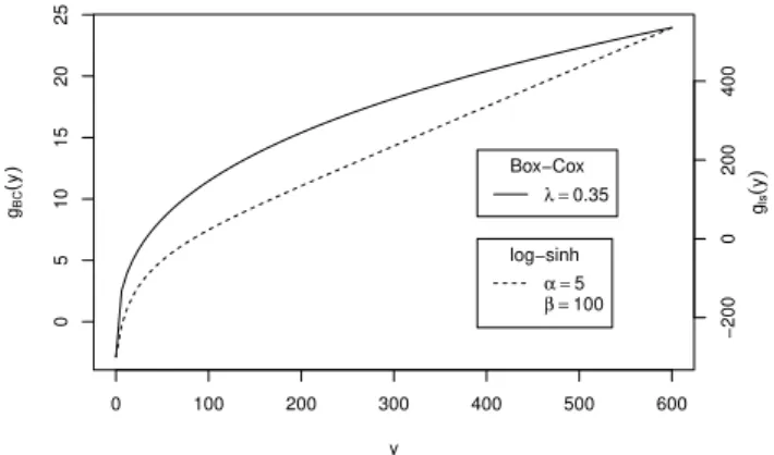
g(y), andzrepresent the transformed output.λis a param-eter that dparam-etermines how strong the transformation is. It is chosen from the interval (0,1), with the extreme cases of 1 leading to the (shifted) identity transformation, and 0 to a log transformation. We choose aλ=0.35, which has lead to satisfactory results in many similar investigations (Willems, 2012; Honti et al., 2013; Yang et al., 2007b, a; Wang et al., 2012; Frey et al., 2011). Assuming a constant variance in the transformed space, this value yields a moderate increase of variance in non-transformed output. This accounts for an ob-served increase in residual variance while keeping the weight of high discharge observations sufficiently high for calibra-tion. In other words, this moderateλassures a good compro-mise between the performances of the error model and the fit of the simulator. The behavior of the Box–Cox transforma-tion and its derivative for the stormwater runoff in our study are shown in Figs. 1 and S1.
Log-sinh
The log-sinh transformation has recently shown very promis-ing results for hydrological applications (Wang et al., 2012). In contrast to the original notation, we prefer a reparam-eterized form with parameters that have a more intuitive meaning:
g(y)=βlogsinh α+y
β
, (14)
g−1(z)=arcsinh exp(z
β)
−α
β
β, (15)
dg
dy =coth
α+y
β
, (16)
whereα(originallya/b) andβ(originally 1/b) are lower and upper reference outputs, respectively.αcontrols how the rel-ative error increases for low flows. For outputs larger thanβ,
❉✐s❝✉ss✐♦♥
P
❛♣
❡r
⑤
❉✐s❝✉ss✐♦♥
P
❛♣
❡r
⑤
❉✐s❝✉ss✐♦♥
P
❛♣
❡r
⑤
❉✐
s❝✉ss
✐♦♥
P
❛♣
❡r
⑤
0 100 200 300 400 500 600
0
5
10
15
20
25
y gBC
(
y
) Box−Cox
λ =0.35
log−sinh
α =5
β =100
−200
0
200
400
gls
(
y
)
Fig. 1.Behavior of the Box–Cox (solid line) and log-sinh (dashed line) transformation as a function of the output variable (e.g., dis-charge in L s−1) with parameters used in this study.
instead, the absolute error gradually stops increasing and the scaling of the error (derivative ofg) becomes approximately equal to unity. In our study, we choseαto be a runoff in the range of the smallest measured flow andβto be an interme-diately high discharge above which uncertainty was assumed not to significantly increase. These considerations are also in agreement with the transformation parameter values deter-mined by Wang et al. (2012). Given the characteristics of our catchment and model we setα=5 L s−1andβ=100 L s−1. The graphs of the transformation function and its derivative with these parameter values are provided in Figs. 1 and S1.
Both transformations are able to reduce the heteroscedas-ticity of residuals, which represents the fact that flowmeters and rating curves are more inaccurate during high flows and systematic errors lead to a higher uncertainty during high flows. Another positive characteristic is that these transfor-mations make error distributions asymmetric, substantially reducing the proportion of negative flow predictions, which can otherwise occur during error propagation.
2.2 Inference and predictions
2.2.1 Prior definition
First, one has to define the joint prior distribution of the parameters of the hydrological model, θ, and of the error model,ψ. In particular, this requires an informative prior of the covariance matrix of the flow measurements. Although a first guess can be obtained from manufacturer’s specifica-tions, it is recommended to assess it separately with redun-dant measurements (see Dürrenmatt et al., 2013). As stated in Sect. 2.1.2, it is important that the prior of the bias reflects the desire to avoid model inadequacy as much as possible. This is obtained by a probability density decreasing with increasing values ofσBct andκ (e.g., an exponential distribution). This
helps to reduce the identifiability problem between the deter-ministic model and the bias. For the prior forσBct, one could
take into account that the maximum bias scatter is unlikely to be higher than the observed discharge variability. On the other hand, the maximum value ofκ is in the same order of magnitude as the maximum discharge divided by the corre-sponding maximum precipitation of a previously monitored storm event. Additionally,τ should represent the character-istic correlation length of the residuals and could be approx-imately set to 1/3 of the hydrograph recession time. More prior information may be available from previous model ap-plications to the same or a similar hydrological system. Fi-nally, the parameters of the chosen transformation have to be specified. These parameters influence the priors ofσE,σBct,
andκ, which are defined in the transformed space.
We recognize that assigning priors for bias parameters might be challenging. Therefore we suggest testing a pos-teriori the sensitivity of the updated parameter distributions to the priors. We advise against using uninformative uniform priors for two reasons. First, as discussed above, our igno-rance about bias parameters is not total. Second, if one lacks knowledge aboutψ one should also lack knowledge about
ψ2, but no distribution exists that is uniform on bothψ and
ψ2(Christensen et al., 2010).
2.2.2 Bayesian inference
Second, the posterior distribution of the simulator and the er-ror model parametersf (θ,ψ|yo,x)is calculated using the
prior distribution,f (θ,ψ), the likelihood function, f (yo| θ,ψ,x), and the observed data, yo, according to Bayes’
theorem:
f (θ,ψ|yo,x)=
f (θ,ψ)f (yo|θ,ψ,x) RR
f (θ′,ψ′)f (y
o|θ′,ψ′,x)dθ′dψ′
. (17)
In other words, during a Bayesian calibration, the joint probability density of parameter and model results, the prod-uct of the prior of the parameters and the likelihood, is con-ditioned on the data.
In order to cope with analytically intractable multi-dimensional integrals, such as the ones in the denominator of Eq. (17) or those raising when marginalizing the joint
posterior, numerical techniques have to be applied. In this context, Markov Chain Monte Carlo (MCMC) simulations are useful for approximating properties of the posterior dis-tribution based on a sample, even if the normalization con-stant in Eq. (17) is unknown. Details are given in Sect. 3.2.
2.2.3 Predictions for the calibration layoutL1
Third, one has to compute posterior predictive distributions for the observations that have been used for parameter esti-mation. The experimental layout of this data set (here: cali-bration layout),L1, specifies which output variables are
ob-served, where and when. Here, the model output at calibra-tion layoutL1 is given by the vector yL1 =(yts1, . . ., y
s tn1),
whereys denotes the discharge at the location,s, of the mea-surements and ti, for i=1, . . . , n1, the time points of the
measurements.
In order to separate different uncertainty components, we compute predictions from (i) the simulatoryL1
M, which only
contains uncertainty from hydrological model parameters; (ii) our best knowledge about the system responseg−1(y˜L1
M+
BL1
M), which comprehends additional uncertainty from input
errors and structural deficits; and (iii) observations of the sys-tem response,g−1(y˜L1
M+B
L1
M+EL1), which, in addition,
in-cludes random flow measurement errors (note that we mean here the application of the scalar functiong−1to all compo-nents of the vector specified as its argument). Usually, hy-drological “predictions” describe simulation results for time points or locations where we do not have measurements. Here, consistent with Higdon et al. (2005) and Reichert and Schuwirth (2012), “predictions” designate the generation of model outputs (with uncertainty bounds) in general.
To obtain probabilistic predictions for multivariate nor-mal distributions involved in the evaluation of these random variables, the reader is referred to Kendall et al. (1994) and Kollo and von Rosen (2005). Taking as an example the pos-terior knowledge of the true system output without obser-vation error conditional on model parameters, the expected transformed values are given by
Ehy˜L1
M +B
L1
M | ˜Y
L1 o ,θ,ψ
i
=
˜
yL1
M +6BL1
M
6EL1+6
BLM1
−1
·y˜L1 o − ˜y
L1
M
(18) and their covariance matrix by
Var ˜
yL1
M +B
L1
M | ˜Y
L1 o ,θ,ψ
=6
BL1 M
6EL1+6
BL1 M
−1
6EL1.(19)
To obtain the posterior predictive distribution of the bias-corrected output, y˜L1
M +B
L1
M, first, we have to propagate a
large sample from the posterior distribution through the sim-ulator, yL1
M, and draw realizations of y˜
L1
M +B
L1
M by using
4216 D. Del Giudice et al.: Improving uncertainty estimation in urban hydrology
uncertainty intervals of this distribution, we compute the sample quantile intervals (e.g., 0.025, 0.5, and 0.975 quan-tiles). A similar procedure has to be applied to derive the predictive distributions ofyL1
M andy˜
L1
M +B
L1
M +EL1.
Besides calculating the posterior predictive distribution, it is important to check the assumptions of the likelihood func-tion. As our posterior represents our knowledge of system outcomes, bias and observation errors, of which not all have a frequentist interpretation, we cannot apply a frequentist test to the residuals of the deterministic model at the best guess of the model parameters. However, we can perform a frequen-tist test based on our knowledge of the observation errors. This makes it necessary to split the residuals into bias and observation errors and to derive the posterior of the observa-tion errors alone. A numerical sample of this posterior can be gained by substituting the sample for the random variable
˜
yL1
M +B
L1
M in
EL1= ˜yL1
o − ˜y L1
M(x,θ)+B L1
. (20)
In this equationy˜L1
o refers to the field data. The medians of
the components of this sample represent our best point esti-mates of the observation errors that we will use to test the statistical assumptions as described in Sect. 2.2.5.
2.2.4 Predictions for the validation layoutL2
Fourth, one computes posterior predictive distributions for the extrapolation layout,L2, where data are not available or
not used for calibration. If data are available, they can be used for validation. In our study,L2denotes the location and
the time points of the extrapolation range, and the associated model output is given byyL2=(ys
tn1+1, . . ., y s
tn2). This
lay-out, however, could also contain interpolation points between calibration data.
A sample for layoutL2 could be calculated similarly to
the one forL1by using Eqs. (35) and (36) of Reichert and
Schuwirth (2012) instead of Eqs. (18) and (19). However, the specific form of our bias formulation as an Ornstein– Uhlenbeck process (Eqs. 5, 7) offers a potentially more ef-ficient alternative. As the OU process is a Gauss–Markov process, we can draw a realization for the entire period by iteratively drawing the realization for the next time step at timetj from that of the previous time step at timetj−1from
a normal distribution. The expected value and variance of the normal distribution of the bias given the model parameters is given by
EhBL2 M,j|B
L2
M,j−1=bj−1,θ,ψ
i
=bj−1·exp
−1t
τ
, (21)
VarhBL2 M,j|B
L2
M,j−1,θ,ψ
i
=
σB2
ct+ κxj−d
2
·
1−exp −21t
τ
. (22)
The sample of the bias forL2can be generated by drawing
iteratively from these distributions for all required values of
j starting from the last result of each sample point from lay-outL1. By calculating the results of the deterministic model
and drawing from the observation error distribution, samples foryL2
M,g−1(y˜
L2
M+B
L2
M), andg−1(y˜
L2
M+B
L2
M+EL2)can be
constructed similarly as for layoutL1.
2.2.5 Performance analysis
Fifth, the quality of the predictions is evaluated by assessing (i) the coverage of prediction for the validation layout and (ii) whether the statistical assumptions underlying the error model are met for the calibration layout.
Checking the predictive capabilities
The predictive capability of the model can be assessed by two metrics, the “reliability” and the “average bandwidth” (Breinholt et al., 2012). The reliability measures what per-centage of the validation data are included in the 95 % credi-bility intervals ofg−1(y˜M+BM+E). When this percentage
is larger than or equal to 95 %, the predictions are reliable. In general we expect this percentage to be larger than 95 % as our uncertainty bands describe our (lack of) knowledge about future predictions. This combines Bayesian paramet-ric and bias uncertainty with the uncertainty due to the ob-servation error. These three components of predictive inter-vals are thus systematically more uncertain than the obser-vation error alone. The limiting case of an exact coverage is only expected to occur if parameter uncertainty and bias is small compared to the observation error. In contrast, the av-erage bandwidth (ABW) measures the avav-erage span of the 95 % credibility intervals. Ideally, we seek the narrowest re-liable bands. Besides these two criteria, the Nash–Sutcliffe efficiency index (Nash and Sutcliffe, 1970), a metric often used in hydrology, is applied to evaluate goodness of fit of the deterministic model to the data.
As a side note, it has been suggested to check the pre-diction performance of a model by examining the number of data points included in the prediction uncertainty intervals re-sulting only from parameter uncertainty (Dotto et al., 2011). Unfortunately, this is not conclusive because the field obser-vations are not realizations of the deterministic model but of the model plus the errors.
Checking the underlying statistical assumptions
term. As outlined in Sect. 2.2.3, we can use the median of the posterior of the observation error at layoutL1to do such
a frequentist test. One should test whether these observation errors are (i) normally distributed, (ii) have constant variance and (iii) are not autocorrelated. As the observation errors may only represent a small share of the residuals of the determin-istic model, posterior predictive analysis based on indepen-dent data, as outlined in the previous paragraph, remains an important performance measure.
As a side note, it is conceptually incorrect to check fre-quentist assumptions by using the full (Bayesian) posterior distribution (e.g., Renard et al., 2010). Using the full pos-terior instead of the best point estimate of the observation errors adds additional uncertainty from the imprecise prior knowledge of parameter values. In our view, this distorts the interpretation of frequentist tests.
2.2.6 Improving the simulator
Finally, after performance checking, one should evaluate the opportunity to improve the simulator and/or the measure-ment design for the model’s input. Hints for improvemeasure-ment can be obtained by exploratory analysis of the bias, for exam-ple by investigating the relation between its median and out-put variables or inout-put. On the one hand, systematic patterns in the relation of the bias to model input or output would suggest the presence of model structural deficits that could be corrected. On the other hand, increasing variance of the bias with increasing discharge could be a sign of excessive uncertainty in rainfall data. This could be improved by more reliable rainfall information.
3 Material
To demonstrate the applicability and usefulness of our ap-proach, we evaluate the performance of nine different error models in a real-world urban drainage modeling study. In the following we will briefly describe the case study and details on the numerical implementation of the bias framework.
3.1 Case study
We tested the uncertainty analysis techniques on a small ur-ban catchment in Sadová, Hostivice, in the vicinity of Prague (CZ). The system has an area of 11.2 ha and is drained by a separate sewer system. It is a green residential area with an average slope of circa 2 %.
The monitoring data of rainfall and runoff were collected in summer 2010 (Bareš et al., 2010). Flow was measured at the outlet of the stormwater system in a circular PVC pipe with a diameter of 0.6 m. A PCM Nivus area-velocity flowmeter was used to record water level and mean velocity every 2 min. These output data show that the hydrosystem is extremely dynamic, with a response ranging approximately
Fig. 2.Aerial photo of our Sadová case study catchment. The map shows the layout of the main stormwater conduits and the location of the rain gauges and the flowmeter.
from 2 L s−1during dry weather to 600 L s−1during strong rainfall.
Rainfall intensities were measured with two tipping bucket rain gauges that were installed only a few hundred meters from the catchment (Fig. 2). These two input temporal data sets have been aggregated to 2 min time steps using inverse distance weighting.
For model calibration, we selected two periods with 6 ma-jor rainfall events. One on 27 August between 01:52 LT and 12:58, and the second in July between 22 July at 23:32 and 23 July at 19:00. For validation, a single period from 23 July at 19:02 to the next day at 07:00 was selected. Calibration and validation storms had a maximum rain rate ranging from 13 to 65 mm h−1and from 8 to 34 mm h−1, respectively. The monitored rainstorms had a duration of 0.5–4 h with a cumu-lative height varying from 2.3 to 33 mm. The calibration and validation data of July 2010 are illustrated in Fig. 4.
3.2 Model implementation
We modeled runoff in the stormwater system using the SWMM software (Rossman and Supply, 2010). The model was set to a simple configuration, namely a nonlinear reser-voir representing the catchment connected to a pipe with a constant groundwater inflow. Lumped modeling is particu-larly appropriate when a study focuses on outlet discharge and computation can be a limiting factor (Coutu et al., 2012). The parameters that we inferred during calibration were the imperviousness, the width, the dry weather inflow, the length of the conduit and the slope of the catchment.
The procedure outlined in Sect. 2.2 to compute the poste-rior predictive distributions was implemented inR(R Core
4218 D. Del Giudice et al.: Improving uncertainty estimation in urban hydrology
❉✐s❝✉ss✐♦♥
P
❛♣
❡r
⑤
❉✐s❝✉ss✐♦♥
P
❛♣
❡r
⑤
❉✐s❝✉ss✐♦♥
P
❛♣
❡r
⑤
❉✐
s❝✉ss
✐♦♥
P
❛♣
❡r
⑤
Q [l/s]
Transformation
log−sinh Box−Cox
none
Bias descr
iption
Input−dep.
Constant
none
time
0
200
400
600
●●●●●●●●●●●●●●●●●● ● ● ● ●●●●●●●●●●●●●●●●●●●●
● ● ● ● ● ● ● ●
●
●
●●●●●●●●●●●●●●●●●● ● ● ● ●●●●●●●●●●●●●●●●●●●●
● ● ● ● ● ● ● ●
●
●
●●●●●●●●●●●●●●●●●● ● ● ●
●●●●●●●●●●●●●●●●●●●● ● ● ● ● ● ● ● ●
●
●
Q [l/s]
0
200
400
600
●●●●●●●●●●●●●●●●●● ● ● ● ●●●●●●●●●●●●●●●●●●●●
● ● ● ● ● ● ● ●
●
●
●●●●●●●●●●●●●●●●●● ● ● ● ●●●●●●●●●●●●●●●●●●●●
● ● ● ● ● ● ● ●
●
●
●●●●●●●●●●●●●●●●●● ● ● ●
●●●●●●●●●●●●●●●●●●●● ● ● ● ● ● ● ● ●
●
●
18:00 19:00 20:00
0
200
400
600
Q [l/s]
●●●●●●●●●●●●●●●●●● ● ● ● ●●●●●●●●●●●●●●●●●●●●
● ● ● ● ● ● ● ●
●
●
18:00 19:00 20:00
●●●●●●●●●●●●●●●●●● ● ● ● ●●●●●●●●●●●●●●●●●●●●
● ● ● ● ● ● ● ●
●
●
18:00 19:00 20:00
●●●●●●●●●●●●●●●●●● ● ● ●
●●●●●●●●●●●●●●●●●●●● ● ● ● ● ● ● ● ●
●
●
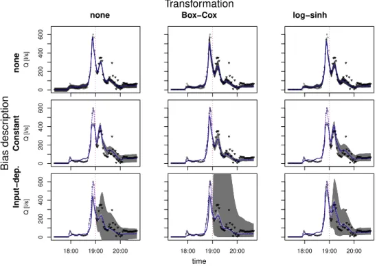
Fig. 3.The 95 % credible intervals for flow predictions for the transition phase obtained with different assumptions on error distribution. The vertical dotted line divides the calibration layout (past) from the validation layout (future). The solid line is the deterministic model output with the optimized parameter set, whereas the dashed line is the bias-corrected output representing our best estimation of the true system response. Observed output of the system is represented by circles and triangles. Triangles were only used to validate the model. Colors of the credibility intervals: deterministic model predictions (light gray), predictions of the real system output (intermediate gray), predictions of new observations (dark gray). When considering bias, the contribution of uncorrelated observation errorsEto total uncertainty becomes very small (.1 L s−1) and therefore is not visible at this scale. Consequently, the credibility intervals for the system output (g−1(y˜M+BM))
and the observations (g−1(y˜M+BM+E)) are almost identical and overlap.
1987).awkwas also used to extract the runoff time series
from the output file.
From a numerical viewpoint, we solved the “inverse prob-lem” described in Sect. 2.2.2 by using a Metropolis–Hastings MCMC algorithm (Hastings, 1970). Before sampling from
f (θ,ψ|yo,x), we obtained a suitable jump distribution
(a.k.a. transition function or proposal density) by using a stochastic adaptive technique to draw from the posterior (Haario et al., 2001). For better performance we added a size-scaling step, which depends on the target acceptance rate. For our inference problem, this algorithm proved to be more ro-bust than others, such as Vihola (2012). However, research on efficient techniques for posterior sampling is evolving rapidly and other approaches could also be used. See Liang et al. (2011) and Laloy and Vrugt (2012) for recent develop-ments in Bayesian computation.
4 Results
In general, accounting for model bias produced substantially wider prediction uncertainty bands in the extrapolation do-main and separated them in three components. The bias
error models also substantially reduced the magnitude of the identified independent observation errors and decreased their autocorrelation. The different formulations of model inade-quacy, however, show a considerable variability in terms of predictive distributions and behavior of the identified obser-vation errors.
4.1 Evaluating the performance of probabilistic sewer
flow predictions
As expected, the different assumptions underlying the nine error models lead to different credibility intervals for stormwater runoff at the monitoring point (Fig. 3, Table 1). Predictions did not exhibit considerable sensitivity to the prior for the bias (results not shown).
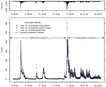
For our case study, the best error model clearly was the constant bias model with log-sinh transformation (Fig. 4). It leads to a high reliability, Nash–Sutcliffe index and sharp total uncertainty intervals.
error model has a 95 % interquantile range up to∼140 L s−1, which is about 32 % of the maximum runoff modeled in the extrapolation phase.
In general, we found that most of the error formulations with model bias produced reliable predictions and around 95 % or more of validation data fell within the 95 % predic-tion interval range for new observapredic-tions (Table 1). In addi-tion, the bias framework separated the total uncertainty into parametric uncertainty, effect of input plus structural deficits, and observation errors (Figs. 3, 4). All the autoregressive er-ror models indicated that most of the predictive uncertainty is due to model bias. Interestingly, uncertainty due to random measurement noise is generally so small that it is not visible in the plots.
In contrast, all error models that ignore model bias, with or without transformation, generated overconfident predictions with too narrow uncertainty bands. As previously stated, they also could not separate the total uncertainty into the individ-ual error contributions.
Besides providing reliable estimates of the total predic-tive uncertainty, a second advantage of the bias framework is that it takes into account the different knowledge within the calibration and validation layouts. As shown in Fig. 3, the predictions obtained with bias description for the calibra-tion layout, to the left of the dotted line, included most of the observations while being, at the same time, very narrow. This takes into account that in the calibration range, where data are available, our knowledge on stormwater runoff is rather accurate and precise. In contrast, for the extrapolation domain where no observations are available, the uncertainty intervals are much larger.
In addition, we found that the conditioning on the monitor-ing data became increasmonitor-ingly weak the further the model pre-dicts into the future. This gradually increases the uncertainty in the transition phase as the prediction horizon moves from the past into the future. Again, this is not possible with the traditional error models. Indeed, models with uncorrelated error terms cannot describe the propagation of information obtained from calibration data to nearby time points. There-fore, their prediction intervals are equally wide for both the calibration and validation layouts.
A third advantage of bias description is that it provides an estimate of the most probable system responseg−1(y˜M+
BM), which is depicted by the dashed line in Fig. 3. In the
calibration layout it closely follows the observations, which are comparably precise and therefore contain the best infor-mation on the state of the system. For the extrapolation lay-out, this information is lacking. However, instead of abruptly reverting to the simulator, the transition is gradual because the autocorrelated bias carries the information from the last monitoring data into the future. This “de-correlation” typi-cally takes a few correlation lengths (here circa 30–50 min).
As can be seen in Table 1 and Fig. 3, even though the uncertainty intervals are more reliable when bias is consid-ered, the deterministic model performs best when residual
P
❛♣
❡r
⑤
❉✐s❝✉ss✐♦♥
P
❛♣
❡r
⑤
❉✐s❝✉ss✐♦♥
P
❛♣
❡r
⑤
❉✐
s❝✉ss
✐♦♥
P
❛♣
❡r
⑤
Fr 00:00 Fr 05:00 Fr 10:00 Fr 15:00 Fr 20:00 Sa 01:00 Sa 06:00
0.020
0.005
I [mm/s]
Fr 00:00 Fr 05:00 Fr 10:00 Fr 15:00 Fr 20:00 Sa 01:00 Sa 06:00
0
100
200
300
400
500
600
Q [l/s]
Uncertainty Bands cred. int. of predicted observations cred. int. of predicted system output cred. int. of model predictions model at posterior's median
Extrapolation layout (L2)
Calibration layout (L1)
Fig. 4.Probabilistic runoff predictions for part of the calibration (left) and the validation period (right) with the constant bias model and log-sinh transformation. The input time series (hyetograph) is shown on the top. The observed hydrograph is represented by dots, with the triangular data points being used only for validation. The 95 % credible intervals are interpreted as follows: parametric uncer-tainty due toyM (light gray), parametric plus input and structural
uncertainty due tog−1(y˜M+BM)(intermediate), total uncertainty
due tog−1(y˜M+BM+E)(dark gray). Validation data not included
in this dark gray region are marked in red. The prediction intervals for the system output and the observations are almost indistinguish-able and therefore only the intermediate gray band is visible at this scale.
autocorrelation and heteroscedasticity are not taken into ac-count. This is not surprising since maximizing the posterior with the simple iid error model with no transformation cor-responds to minimizing the sum of the squares of the errors and therefore produces the best fit.
Comparing the input-independent and dependent bias for-mulations, two important points are observed. First, the con-stant bias description produced on average narrower uncer-tainty bands than the input-dependent version. The latter, in particular, produced huge uncertainties during rain events and very narrow intervals during dry weather. Second, as ex-pressed in Table 1, the constant bias almost produced the same simulator fit as the simple error model, whereas the input-dependent bias formulation performed on average less satisfactorily.