Variability and trends in dynamical forcing of tropical lower stratospheric temperatures

(1)

ACPD

14, 13381–13412, 2014

Tropical stratosphere trends

S. Fueglistaler et al.

Title Page

Abstract Introduction

Conclusions References

Tables Figures

◭ ◮

Back Close

Full Screen / Esc

Printer-friendly Version Interactive Discussion

Discussion

P

a

per

|

Discus

sion

P

a

per

|

Discussion

P

a

per

|

Discussion

P

a

per

|

Atmos. Chem. Phys. Discuss., 14, 13381–13412, 2014 www.atmos-chem-phys-discuss.net/14/13381/2014/ doi:10.5194/acpd-14-13381-2014

This discussion paper is/has been under review for the journal Atmospheric Chemistry and Physics (ACP). Please refer to the corresponding final paper in ACP if available.

Variability and trends in dynamical forcing

of tropical lower stratospheric

temperatures

S. Fueglistaler1, M. Abalos2, T. J. Flannaghan1, P. Lin3, and W. J. Randel4

1

Department of Geosciences/Program in Atmospheric and Oceanic Sciences, Princeton University, Princeton, USA

2

Laboratoire de Météorologie Dynamique, Paris, France

3

Geophysical Fluid Dynamics Laboratory, Princeton, USA

4

NCAR/UCAR, Boulder, CO, USA

Received: 7 April 2014 – Accepted: 11 May 2014 – Published: 23 May 2014 Correspondence to: S. Fueglistaler (stf@princeton.edu)

(2)

ACPD

14, 13381–13412, 2014

Title Page

Tables Figures

◭ ◮

Back Close

Full Screen / Esc

Discussion

P

a

per

|

Discus

sion

P

a

per

|

Discussion

P

a

per

|

Discussion

P

a

per

|

Abstract

We analyse the relation between tropical lower stratospheric temperatures and dy-namical forcing over the period 1980–2011 using NCEP, MERRA and ERA-Interim re-analyses. The tropical mean thermodynamic energy equation with Newtonian cooling for radiation is forced with two dynamical predictors: (i) the average eddy heat flux of

5

both hemispheres; and (ii) tropical upwelling estimated from momentum balance fol-lowing Randel et al. (2002). The correlation (1995–2011) for deseasonalised tropical average temperatures at 70 hPa with the eddy heat flux based predictor is 0.84 for ERA-Interim (0.77 for the momentum balance calculation), and 0.87 for MERRA. The eddy heat flux based predictor indicates a dynamically forced cooling of the tropics

10

of ∼ −0.1 K decade−1 (∼ −0.2 K decade−1 excluding volcanic periods) for the period 1980–2011 in MERRA and ERA-Interim. ERA-Interim eddy heat fluxes drift slightly rel-ative to MERRA in the 2000’s, possibly due to onset of GPS temperature data assimi-lation. While NCEP gives a small warming trend, all 3 reanalyses show a similar sea-sonality, with strongest cooling in January/February (∼ −0.4 K decade−1, from

north-15

ern hemispheric forcing) and October (∼ −0.3 K decade−1, from southern hemispheric

forcing). Months preceding and following the peaks in cooling trends show pronounced smaller, or even warming, trends. Consequently, the seasonality in the trends arises in part due to a temporal shift in eddy activity. Over all months, the Southern Hemisphere contributes more to the tropical cooling in both MERRA and ERA-Interim. The residual

20

time series (observed minus estimate of dynamically forced temperature) are well cor-related between ERA-Interim and MERRA, with differences largely due to temperature differences. The residual time series is dominated by the modification of the radiative balance by volcanic aerosol following the eruption of El Chichon (maximum warming of∼3 K at 70 hPa) and Pinatubo (maximum warming of∼4 K at 70 hPa), with a strong

25

(3)

ACPD

14, 13381–13412, 2014

Title Page

Tables Figures

◭ ◮

Back Close

Full Screen / Esc

Discussion

P

a

per

|

Discus

sion

P

a

per

|

Discussion

P

a

per

|

Discussion

P

a

per

|

1 Introduction

Temperature trends in the lower stratosphere over the last few decades are substan-tially larger than predicted by General Circulation Models (GCMs) forced with increas-ing greenhouse gases only (Ramaswamy et al., 2006). Consequently, trends in strato-spheric dynamics and other radiatively active trace constituents (such as ozone) may

5

play a major role for temperature trends in this layer, and decomposition into dynami-cally and radiatively forced trends has attracted much interest (see e.g. recent analyses of Fu et al., 2010; Ueyama and Wallace, 2010; Bohlinger et al., 2014). The much im-proved availability of vertically resolved atmospheric composition measurements since the 1980’s, and the availability of meteorological reanalyses allows a more detailed

10

analysis based on observations than what would be possible if only temperature mea-surements were available. However, systematic errors in the time series of any of the relevant quantities (temperature, radiatively active trace constituents, and atmospheric dynamics) have prevented definitive attribution of observed trends. For example, Free (2011) provides an overview of uncertainties in temperature trends from a range of

15

different radiosonde data homogenisation efforts, and Solomon et al. (2012) show that the new ozone dataset of Hassler et al. (2013) gives much larger cooling trends (due to ozone alone) than older ozone data sets. Similarly, estimation of trends in the dynam-ical forcing relies ultimately in one way or another on information from meteorologdynam-ical reanalyses, and the purpose of this paper is to document common features and diff

er-20

ences therein in several modern reanalyses.

We focus on the relation between lower stratospheric eddy heat fluxes and tropical lower stratospheric temperatures for the period 1980–2011 as represented in reanal-yses. Specifically, we document in detail the time series of this relation, and discuss differences among different reanalyses, and differences in two different methods to

re-25

(4)

ACPD

14, 13381–13412, 2014

Title Page

Tables Figures

◭ ◮

Back Close

Full Screen / Esc

Discussion

P

a

per

|

Discus

sion

P

a

per

|

Discussion

P

a

per

|

Discussion

P

a

per

|

as ozone and water vapour change due to processes not directly coupled to dynamics. In reanalyses, the relation may be also distorted by changes in the assimilated data since the assimilation system is not required to conserve energy (see e.g. discussion in Fueglistaler et al., 2009a).

Our analysis focuses on the level around 70 hPa. The Microwave Sounding Unit

5

(MSU) channel 4 (also referred to as “Temperature of the Lower Stratosphere”, TLS) temperature measurements are centered near that level, which provides some sta-bility to temperatures and eddy heat fluxes at this level in reanalyses which typically assimilate this data. The TLS time series is considered to be of high quality, but may suffer also from smaller artefacts. Further, we document the relation between the 70

10

and 100 hPa eddy heat fluxes in reanalyses. Archived results from GCM comparison projects such as the SPARC CCMVal initiative (SPARC CCMVal, 2010) often archive only eddy heat fluxes at 100 hPa, which then have to serve as dynamical proxy for the entire lower stratosphere.

The use of extra-tropical eddy heat fluxes at a specific level as indicator for

strato-15

spheric dynamics, and its role for tropical temperatures, is an oversimplifcation that is primarily justified by (i) the ease of computation, and the fact that it often is the only dynamical information archived in model intercomparison projects; (ii) a relatively straightforward error analysis due to the simple calculation; and (iii) it works empirically remarkably well.

20

In addition to the simple temperature proxy based on eddy heat fluxes, we calculate an estimate of temperature variations based on the tropically averaged upward mass flux using the momentum balance equation of Randel et al. (2002), whereby we use for the conversion from vertical mass flux to temperature the Newtonian cooling approxi-mation and the (well justified) assumption that latitudinal heat fluxes out of the tropics

25

are much smaller than vertical advection over the whole tropics.

(5)

ACPD

14, 13381–13412, 2014

Title Page

Tables Figures

◭ ◮

Back Close

Full Screen / Esc

Discussion

P

a

per

|

Discus

sion

P

a

per

|

Discussion

P

a

per

|

Discussion

P

a

per

|

errors, (ii) errors in the dynamical information, (iii) missing processes such as forcing from unresolved waves, and tropical waves that may be resolved but not included in the dynamical information of the eddy heat flux proxy, and (iv) changes in radiative condi-tions not correlated with the changes in dynamics as represented by the dynamical proxies.

5

With the focus on the time series, identification of possible reasons for differences in trends, and in particular discussion of the evolution of the relation between two related quantities – dynamical forcing and temperatures – this paper complements related studies such as the comparison of the stratospheric circulation in reanalyses presented by Iwasaki et al. (2009), the detailed analyses of the stratospheric circulation in

ERA-10

Interim by Seviour et al. (2012), or studies of trends in stratospheric age of air based on reanalyses (Diallo et al., 2012).

2 Method

2.1 Framework

Consider the thermodynamic energy equation in the quasi-geostrophic, transformed

15

Eulerian mean set of equations, and assume that the diabatic heating term can be approximated by Newtonian cooling,

∂T ∂t +(N

2_H/R

)·w∗₌TE −T

τ (1)

(see e.g. Eq. (1) of Yulaeva et al., 1994), whereτis the radiative relaxation time scale,

20

TEis the radiative equilibrium temperature,N 2

is the buoyancy frequency,His the scale height,R is the gas constant,w∗is the diabatic residual velocity,T is temperature, and tis time, and all quantities are zonal means (tropical means in this work).

In this framework, we may force temperature T with w∗

and TE, where variations in

(6)

ACPD

14, 13381–13412, 2014

Title Page

Tables Figures

◭ ◮

Back Close

Full Screen / Esc

Discussion

P

a

per

|

Discus

sion

P

a

per

|

Discussion

P

a

per

|

Discussion

P

a

per

|

w∗ may also affect tracers (here particularly ozone, see e.g. Fueglistaler et al., 2011) and henceTE. It is well known that Newtonian cooling is a relatively poor

approxima-tion for the lower stratosphere (see e.g. the analysis by Hitchcock et al., 2010), but in practice there exist reasonably linear relations between local heating rate, tempera-ture and radiatively active tracer amounts for smooth perturbations with vertical scales

5

similar to that of the lower stratosphere (and longer) (Fueglistaler et al., 2011, 2014). Hence, for the conceptual interpretation of the connection between dynamics, tracers and temperatures, Eq. (1) is sufficient.

Radiative transfer calculations (not shown) show that the first order radiatively active trace constituents that need to be considered are aerosol and ozone; variations with

10

observed magnitudes of water vapor, carbon dioxide and other long-lived greenhouse gases typically affect temperature about an order of magnitude less.

Under the assumption that temperature variations are only dynamically forced (i.e. w∗

in Eq. 1), the equilibrium temperature is constant and the solution for the difference between temperature and equilibrium temperature,∆T(t)≡T_E−T(t), is of the form

15

∆T(t)=f(t)∗h(t) (2)

wheref(t) is the forcing,∗denotes the convolution, and the unit pulse responseh(t)₌0

fort >0 and h(t)=et/τ fort≤0. For the calculation of temperature variability based

on eddy heat fluxes (Sect. 2.3) and estimates of upwelling (Sect. 2.4), the convolution

20

will be evaluated over a length of 3 times the e-folding time scaleτ. Sinceτis of order 100 days (see below), the first year of data (i.e. the year 1979) is not considered in our analyses.

With the focus of this analysis on variability and trends, all calculations shown are based on deseasonalised, monthly mean data. That is, for each month the

climatologi-25

cal mean of that month (determined from detrended data) is subtracted. Since volcanic eruptions lead to major disturbances in the radiative conditions (i.e.TEis not constant),

(7)

ACPD

14, 13381–13412, 2014

Title Page

Tables Figures

◭ ◮

Back Close

Full Screen / Esc

Discussion

P

a

per

|

Discus

sion

P

a

per

|

Discussion

P

a

per

|

Discussion

P

a

per

|

2.2 Data

Temperature and eddy heat flux data are taken from ERA-Interim (Dee et al., 2011), MERRA (Rienecker et al., 2011) and NCEP (Kalnay et al., 1996), with a focus on the 70 hPa level (for ERA-Interim, we use the 67 hPa original model level). For NCEP, we show in the following results for the DOE NCEP-2 data, results with the

5

older NCEP data are very similar. Eddy heat fluxes are calculated from 6 hourly (00:00/06:00/12:00/18:00 UTC) data, at a horizontal resolution of 1◦/1◦ for ERA-Interim, 1.25◦/1.25◦

for MERRA, and 2.5◦/2.5◦

for NCEP.

The reanalysis temperatures are complemented with measurements from the Mi-crowave Sounding Unit (MSU) lower stratospheric channel (“TLS”, also known as MSU

10

channel 4) as provided by RSS (Mears and Wentz, 2009). The TLS channel’s weighting function is centered near 70 hPa, but the deep vertical weighting function is problematic for interpretation of TLS data in the tropics (Fueglistaler, 2012). The data is shown here because it provides a tropical mean without sampling bias, and it has a strong impact on lower stratospheric temperatures in reanalyses.

15

2.3 The proxy for tropical temperatures

The specific proxy used here for the influence of extratropical dynamics on tropical temperatures in the lower stratosphere is motivated by the approach of Newman et al. (2001) for polar vortex temperatures. The proxy was introduced in Fueglistaler (2012), and we provide here a more detailed description and assessment of sensitivities. The

20

proxy is mainly determined by mid-/high latitude eddy heat fluxes, and the basic conclu-sions shown here for this specific proxy do apply also to any other proxy that is based on some averaged mid-/high latitude eddy heat flux. Specifically, the results and con-clusions based on the specific proxy used here should be very similar for 3 month mean eddy heat fluxes averaged between 50 and 10 hPa as done in Fu et al. (2010), 3 month

25

(8)

ACPD

14, 13381–13412, 2014

Title Page

Tables Figures

◭ ◮

Back Close

Full Screen / Esc

Discussion

P

a

per

|

Discus

sion

P

a

per

|

Discussion

P

a

per

|

Discussion

P

a

per

|

100 hPa eddy heat flux index used by Ueyama et al. (2013), or the 100 hPa eddy heat flux integrated from 45–70◦N averaged over 45 days used by Bohlinger et al. (2014).

The proxy used here is the eddy heat flux from 6 hourly data, averaged from the sub-tropics to high latitudes in both hemispheres, and e-folded with a relaxation time scale of about 3 months. Details of the proxy are provided in the appendix, the most relevant

5

aspects are: (i) results shown in the paper are based on the latitude average from 25 to 75◦on both hemispheres. Results are not sensitive to the exact choice of latitudes but must include the range∼40 to∼70◦(i.e the skill of the proxy arises from the mid/high latitude eddy heat fluxes). Note that this implies that the analyses here are limited to the role of the mid/high latitudes, and do not provide insights on tropical and

subtrop-10

ical forcing of the tropical lower stratosphere. (ii) At 70 hPa, results for ERA-Interim, MERRA and NCEP are very similar, but for NCEP the correlation to tropical temper-atures is lower. (iii) At 100 hPa, the proxy differs between ERA-Interim and MERRA (NCEP not discussed) with respect to the role of the subtropics. With the focus on the lower stratosphere here, we do not further discuss this result, but it should be kept in

15

mind for analyses of temperatures around 100 hPa. We do, however, discuss the rela-tion between the 100 and 70 hPa eddy heat fluxes, as in recent model intercomparison projects often only the 100 hPa eddy heat flux was archived. (iv) For ERA-Interim and MERRA, correlations between tropical average temperature and the proxy maximise for relaxation timescales around 80 days with a correlation coe_fficients∼0.85 for the

20

period 1995 to 2011. For NCEP, the corresponding maximum correlation coefficient is 0.75 for a relaxation time scale of∼60 days. For the full period 1980 to 2011, the correlation coe_fficients are only marginally smaller for ERA-Interim and MERRA when excluding volcanic periods (the warming due to the volcanic aerosol dominates tropical temperatures during these periods). Results are insensitive to variations of 10 to 20

25

days in relaxation time scale.

(9)

ACPD

14, 13381–13412, 2014

Title Page

Tables Figures

◭ ◮

Back Close

Full Screen / Esc

Discussion

P

a

per

|

Discus

sion

P

a

per

|

Discussion

P

a

per

|

Discussion

P

a

per

|

temperature and the e-folded average eddy heat flux (based on Eqs. 1 and 2),

Tp(t)=α·[v

′ T′

]75₂₅(t)∗h(t) (3)

whereTpis the proxy time series,v

′ T′

is the eddy heat flux, and the operator [·]75₂₅ is the zonal mean averaged between 25 and 75◦ latitude on both hemispheres. As before,

5

∗denotes the convolution, and h(t)=et/τ for t≤0 and h(t)=0 for t >0, withτ∼80 days for ERA-Interim and MERRA, andτ∼60 days for NCEP (see Appendix A2 for

evaluation of the time scale).

Note that the slope obtained from the total least squares regression of the proxy with observed temperatures implies that the proxy Tp also includes the temperature 10

changes from changes inTEdue to tracer variations that are correlated with the proxy

(of particular importance for ozone). In other words, the proxy time seriesTprepresents

the dynamically forced temperature changesincludingcorrelated changes inTE.

The residual,

Tresidual(t)=T(t)−Tp(t) (4)

15

thus represents changes in temperature due to (i) radiative changes inTe from tracer

changes not correlated with dynamics as represented byTp, (ii) errors in the

reanaly-ses’T(t) and eddy heat fluxes, and (iii) errors from dynamical forcing terms not included in the calculation.

20

2.4 Estimate of temperature variations based on momentum balance

In addition to the eddy heat flux proxy, we calculate the zonal mean tropical average upwelling using the momentum balance calculation of Randel et al. (2002). As detailed in Randel et al. (2002), the time-varying zonal mean tropical average upwelling can be calculated from the vertical integral of EP-flux divergence and acceleration at the

25

(10)

ACPD

14, 13381–13412, 2014

Title Page

Tables Figures

◭ ◮

Back Close

Full Screen / Esc

Discussion

P

a

per

|

Discus

sion

P

a

per

|

Discussion

P

a

per

|

Discussion

P

a

per

|

The calculated estimate of the tropical mean residual velocityw∗is converted to tem-perature using again the Newtonian cooling approximation (see Eqs. 1 and 2 above). As before, the relaxation time scaleτis determined by optimizing the correlation with the observed temperature variations (using deseasonalised data). Maximum correla-tion with ERA-Interim is found aroundτ∼70 days, i.e. at a slightly shorter time scale

5

than for the proxy based on the eddy heat fluxes.

The proportionality between the forcingw∗and the temperature response is given by τ,N2and scale heightH. Interestingly, we find that inserting values for these parame-ters typical for the lower stratosphere (N2=6×10−4s−2,H=7000 m andτ=70 days)

gives an amplitude of temperature variations very similar to that observed for the

pe-10

riod 1995–2011. That is, the slope of the total least squares fit between the two time series in this period is 1.02. The implication is that for this period the modification of deseasonalised temperature variations due to variations in TE is actually small, and

the calculation of temperature from upwelling determined with the momentum balance equation not only explains a large fraction of the variability, but also gives the correct

15

amplitude of the temperature variations.

2.5 Removal of QBO variability in tropical temperatures

Tropical stratospheric temperatures are strongly affected by the Quasi–Biennial Oscil-lation (QBO, see e.g. Baldwin et al., 2001), whose forcing is not well resolved in reanal-ysis data. The acceleration of the flow in the inner tropics produces a see-saw pattern

20

in temperature between inner and outer tropics that distorts the relation to meridional eddy heat fluxes. The latitudinal scale of the QBO (order 1000 km) is substantially shorter than the scale of the mid-/high latitude eddy forcing, and this scale separation may be used to reduce the variance in tropical temperatures due to the QBO.

A linear regression analysis of deseasonalised equatorial wind shear with

temper-25

(11)

ACPD

14, 13381–13412, 2014

Title Page

Tables Figures

◭ ◮

Back Close

Full Screen / Esc

Discussion

P

a

per

|

Discus

sion

P

a

per

|

Discussion

P

a

per

|

Discussion

P

a

per

|

chose to define the tropics slightly wider than usual – up to 35◦latitude. Note that this “filtering” assumes a constant length scale of the QBO, which may not always be true. Departures between proxy and temperatures thus not only reflect failure of the proxy to explain the temperature variations related to the eddy heat flux, but may also be a consequence of incomplete filtering of QBO-related variance.

5

3 Results

Figure 1a shows the deseasonalised global average, the tropical average, and the com-bined extratropical average of the RSS microwave sounding unit lower stratospheric channel “TLS”. The strong anti-correlation between tropical and combined extratrop-ical average temperatures is readily visible, though the fact that they nearly perfectly

10

cancel in the global average in response to variations in the strength of the residual circulation is a coincidence (Fueglistaler et al., 2011). Also, the apparent step-wise decrease in global average temperatures (possibly resulting largely from changes in the radiative properties of the stratosphere given the small net impact of dynamical variability) noted by Pawson et al. (1998) is well visible.

15

Figure 1b–d shows the tropical average temperatures near 70 hPa from ERA-Interim, MERRA and NCEP, and the corresponding temperature proxy (Tp) time series. On

in-terannual timescales, the three reanalyses agree well (with better agreement between ERA-Interim and MERRA) in terms of the evolution of temperature and temperature proxy. All time series show relatively small trends from about 1995 onwards, which is

20

why we use the period 1995 to 2011 to determine the slope between proxy and tem-perature, and to calculate the correlation coefficient.

The shape of the time series of temperatures and temperature proxies suggests that linear trend calculations may provide a poor characterisation of the evolution over the last 3 decades. Specifically, the two volcanic eruptions may have an unduly influence

25

(12)

ACPD

14, 13381–13412, 2014

Title Page

Tables Figures

◭ ◮

Back Close

Full Screen / Esc

Discussion

P

a

per

|

Discus

sion

P

a

per

|

Discussion

P

a

per

|

Discussion

P

a

per

|

in the following we will calculate linear trends as a means to quantitatively compare results. We emphasise the uncertainty in these linear trends arising from possible sys-tematic errors in the data, as well as sensitivity to the specific period chosen. Specifi-cally, the start/end date of the period, and volcanic periods have a substantial impact on the linear trends. We account for these uncertainties by providing trends also for

5

variations in start/end date, and for data where 2 years of data following the eruptions of El Chichon and Pinatubo is removed.

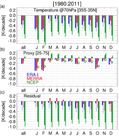
3.1 Temperature trends

Figure 2 shows linear trends for each month separately for ERA-Interim, MERRA and NCEP. Temperature trends (Fig. 2a) are largest for NCEP. The exclusion of the

post-10

volcanic periods has a similar effect on all reanalyses in all months. ERA-Interim and MERRA agree fairly well in January and February, but for the rest of the year ERA-Interim shows stronger cooling. The seasonal distribution of the cooling, with a min-imum during March–June, is similar to that reported by Free (2011) for the average 10◦S–10◦N over the period 1979–2009 of homogenised radiosonde data.

15

3.2 Eddy heat flux trends

All three reanalyses show the strong increase in eddy heat flux following the eruption of Pinatubo in June 1991 noted by Fueglistaler (2012) in ERA-Interim, and are gen-erally well correlated on interannual time scales. For MERRA and ERA-Interim, the difference between tropical average temperature and the proxy shows much less drift

20

over time than for NCEP. Figure 2 shows that most of this difference is due to the much larger temperature trend in NCEP compared to ERA-Interim or MERRA. However, the representation of eddy heat fluxes in the reanalyses further increases this discrepancy as the NCEP proxy shows a weak positive (i.e. warming) trend, while ERA-Interim and MERRA proxies show a cooling trend. For ERA-Interim and MERRA, the trends over all

25

(13)

ACPD

14, 13381–13412, 2014

Title Page

Tables Figures

◭ ◮

Back Close

Full Screen / Esc

Discussion

P

a

per

|

Discus

sion

P

a

per

|

Discussion

P

a

per

|

Discussion

P

a

per

|

Interestingly, the seasonality in the proxy trends in NCEP is actually very similar to that in ERA-Interim and MERRA, which becomes evident after removal of the diff er-ence in the annual mean trend (see Fig. 2b, green diamonds, which are the NCEP monthly trends shifted by the average trend difference to the other reanalyses, i.e. about−0.2 K decade−1).

5

The excellent agreement between MERRA and ERA-Interim for the linear trends over the period 1980–2011 may be slightly fortuitous. Figure 3 shows the differences in the proxy time series between ERA-Interim and MERRA for the 70 and 100 hPa levels. The figure shows that the trend differences between MERRA and ERA-Interim at 70 hPa in Fig. 2b may be due to a small drift between the two reanalysises in the

10

early/mid 2000’s. At 100 hPa, a similar drift but with opposite sign is observed.

It is unclear at this point what exactly causes these drifts between the reanalyses. The ratio between e-folded eddy heat flux at 70 and 100 hPa is relatively stable for MERRA (see Fig. 3b, red line) and NCEP (not shown), but drifts for ERA-Interim in the 2000’s (see Fig. 3b, blue line). Hence, in the “ERA-Interim world” a change in the

15

eddy dissipation between 100 and 70 hPa occurs in the 2000’s, which is not seen in the “MERRA world” or “NCEP world”. A hypothesis is that the onset of assimilation of GPS temperature data in ERA-Interim (from 2000’s onwards CHAMP, and after 2006 COSMIC, Poli et al., 2010; Dee et al., 2011) may induce a drift in ERA-Interim that is not present in MERRA (which does not assimilate these data, Rienecker et al., 2011),

20

and NCEP.

3.3 The dynamical temperature predicted by the momentum balance equation

Figure 4a shows, for ERA-Interim, temperatures at 67 hPa, the temperature proxy based on the eddy heat flux, and temperatures predicted from the upwelling estimate of the momentum balance equation. The figure shows that the two estimates are similar,

25

(14)

ACPD

14, 13381–13412, 2014

Title Page

Tables Figures

◭ ◮

Back Close

Full Screen / Esc

Discussion

P

a

per

|

Discus

sion

P

a

per

|

Discussion

P

a

per

|

Discussion

P

a

per

|

series (i.e. temperature minus proxies). Over the entire period, both residuals are dom-inated by the volcanic signal, which is responsible for the high correlation between the two (r=0.82 for the period 1980 to 2011). For a period without volcanic eruptions, the correlation is much lower (for example for 2000–2011, the correlation isr =0.40; note that we deliberately excluded 1995–2000 here as there is also some drift, further

5

discussed below). Hence, in the absence of strong forcing on the equilibrium temper-ature from volcanic aerosol, the residuals primarily reflect shortcomings of the proxies or errors in temperatures that are not correlated between the two reanalyses.

The two predictors have different trends (0.19±0.05 K decade−1 vs. −0.15±

0.05 K decade−1), which is also clearly visible in the residual (Fig. 4b). The implication is

10

that the trends in the dynamical information in ERA-Interim at the bounding latitudes of 30◦S/30◦N from 67 hPa upwards required for the momentum balance calculation and the eddy heat flux at the 67 hPa level integrated from 25–75◦ on both hemispheres, are statistically significantly di_fferent. This seemingly paradoxical result reflects the fact that both calculations give imperfect estimators of the true dynamical forcing, and that

15

the assimilation system of reanalyses may induce spurious trends that affect different quantities in di_fferent ways. It should be seen as a warning that di_fferences between trend estimates in the literature may not only arise from the use of different datasets, but also that the exact formulation of the quantity used to quantify the dynamical forcing can have a large influence on results as well.

20

Apart from the differences in the trends of the two predictors (which are further dis-cussed below), we note the following: (i) the generally good agreement between the two calculations provides additional support for the empirically determined proxy based on the eddy heat fluxes; and (ii) the momentum balance calculation confirms the large dynamically forced drop in tropical temperatures in October 2000 and the strong

dy-25

(15)

ACPD

14, 13381–13412, 2014

Title Page

Tables Figures

◭ ◮

Back Close

Full Screen / Esc

Discussion

P

a

per

|

Discus

sion

P

a

per

|

Discussion

P

a

per

|

Discussion

P

a

per

|

is actually substantially larger than what one would estimate from analysis of tempera-ture alone.

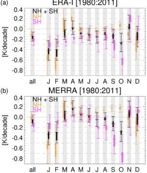
3.4 Hemispheric trends in eddy heat fluxes

Figure 5 shows the trends in the dynamically forced tropical temperature based on the e-folded eddy heat fluxes (for ERA-Interim and MERRA), and the contributions from

5

each hemisphere. As in Fig. 2, the trends are shown for annual mean data, and for each month. The figure shows that results (annual mean, and seasonality) for ERA-Interim (panel a) and MERRA (panel b) are very similar not only for the combined forcing, but also for each hemisphere. The trends for the period 1980–2011 are shown with their 1-sigma uncertainty. We also found that some of the trends have a substantial

10

sensitivity to the start/end time. In order to provide an indicator for this sensitivity, the thick bars show the range of linear trends when varying the start year or end year by 1 year (i.e. they give the minimum/maximum range of trends calculated for the periods 1980–2011, 1981–2011, and 1980–2010).

The figure shows that irrespective of the uncertainty metric, the seasonality in trends,

15

and the hemispheric differences therein, is statistically fairly robust for both ERA-Interim and MERRA. The trends in dynamical forcing originate primarily from the Northern Hemisphere in January and February, and from the Southern Hemisphere in October. For both hemispheres, the peaks in positive trends in dynamical forcing (leading to cooling in the tropics) are followed by a large drop (i.e. warming in the tropics) in the

20

subsequent months (March/April for the Northern Hemisphere, November/December for the Southern Hemisphere). Hence, part of the seasonal pattern in the trend may arise from a temporal shift in eddy activity rather than a general increase in eddy activ-ity. We note that for both ERA-Interim and MERRA the larger contribution to the total forcing on the tropics is from the dynamics of the Southern Hemisphere.

25

(16)

ACPD

14, 13381–13412, 2014

Title Page

Tables Figures

◭ ◮

Back Close

Full Screen / Esc

Discussion

P

a

per

|

Discus

sion

P

a

per

|

Discussion

P

a

per

|

Discussion

P

a

per

|

at 100 and 70 hPa in ERA-Interim but not MERRA after the year 2000 casts some doubt whether the positive trend in ERA-Interim is real even if it is statistically significant.

In Sect. 3.3 we have shown that for ERA-Interim the trend based on the momentum balance calculation differs substantially from that of the dynamical temperature proxy based on eddy heat fluxes. Given that for the eddy heat flux estimate the seasonality

5

is robust among different reanalyses while the mean trend differs, we may ask whether this is also true for the difference between the eddy heat flux estimate and the estimate based on the momentum balance calculation.

Figure 6a shows the mean trends and the trends for each month of the two calcula-tions. It is evident that not only the annual mean is different, but that also the seasonality

10

di_ffers. Figure 6b shows the time series of the two estimates for January and for July, and Fig. 6c shows the difference between the two estimates for each month and year (i.e. the colors in (c) show the difference between the two curves shown in (b), for each month). The pattern in Fig. 6c suggests that there is no simple answer as to why the two estimates differ. There appears to be an overall drift from the pre-2000 period to the

15

post-2000 period, with an anomaly around 1984–1986 in the months April–November. As a result of this anomaly, the monthly trends in the momentum balance estimate are not just a shifted version of those in the eddy heat flux calculation, but have a different seasonality. Further, note that there is some overlap of this period with the post-volcanic period of El Chichon, such that excluding volcanic periods produces a di_fferent change

20

in the linear trends of the two estimates (results not shown).

Given that all three reanalyses have a similar seasonality in the trend of the eddy heat fluxes, and the strong constraints imposed by the MSU-4 data on the 70 hPa level temperatures, we regard these trends to be likely more reliable than those of the momentum balance calculation even though the latter are more physical.

25

3.5 The residual – signal and artefacts

(17)

ACPD

14, 13381–13412, 2014

Title Page

Tables Figures

◭ ◮

Back Close

Full Screen / Esc

Discussion

P

a

per

|

Discus

sion

P

a

per

|

Discussion

P

a

per

|

Discussion

P

a

per

|

changes in the radiative equilibrium temperatureTE. As already noted in the discussion

of the trends in the residual (Fig. 2c), the differences in temperature between the re-analyses are the main source of uncertainty in the residual. NCEP is the outlier and is in all likelyhood the least reliable of the three reanalyses (see also Randel et al., 2004). However, also the differences in the (annual average) trend in the residual between

5

MERRA and ERA-Interim are as large as the trends in either of the two reanalyses (see Fig. 2c).

Visual inspection of the residual time series (Fig. 1d) shows that the time series is dominated by the e_ffect of the two major volcanic eruptions, El Chichon and Pinatubo. Further, the high correlation of the residuals from MERRA and ERA-Interim suggests

10

that on shorter timescales, the variance is due to true failure of the dynamical proxy to capture the temperature variations completely rather than uncertainty in the tempera-ture record. Further analysis of the residual in terms of contributions from changes in radiatively active tracers is beyond the scope of this paper, but the fact that the residual time series of ERA-Interim and MERRA are very similar may provide motivation for

15

further analyses in this direction.

3.6 Substitution with 100 hPa eddy heat flux

We have compared the 70 hPa temperatures with the proxy based on the 70 hPa eddy heat fluxes. However, GCMs often archive 6 hourly data, or eddy heat fluxes, only on 100 hPa due to the accepted role of this level for polar temperatures (Newman et al.,

20

2001). Calculating the proxy based on eddy heat flux at a lower layer gives additional errors if the ratio between the eddy heat fluxes of the two layers varies over time, i.e. if the dissipation between the two layers varies. As discussed above, Fig. 3b shows that in ERA-Interim the ratio of 100 to 70 hPa eddy heat fluxes drifts relative to that in MERRA, with the consequence that trends calculated with 100 hPa eddy heat fluxes

25

(18)

ACPD

14, 13381–13412, 2014

Title Page

Tables Figures

◭ ◮

Back Close

Full Screen / Esc

Discussion

P

a

per

|

Discus

sion

P

a

per

|

Discussion

P

a

per

|

Discussion

P

a

per

|

as for the eddy heat fluxes at 70 hPa. Hence, we conclude that for many practical pur-poses the 100 hPa eddy heat fluxes may be taken for the dynamical proxy, not least also because we suspect that the divergence between the two levels in ERA-Interim may be a result of a change in assimilated observations; a problem that does not affect free running GCMs.

5

4 Conclusions

We have analysed the relation between tropical lower stratospheric temperatures (with a focus on 70 hPa) and dynamical forcing of temperature using NCEP, MERRA and ERA-Interim data. We find that a simple proxy based on the extratropical eddy heat flux of both hemispheres e-folded with a timescale of about 80 days gives a very high

10

correlation (with correlation coefficients around 0.85) with observed temperature vari-ability. The more physical calculation of upwelling based on momentum conservation following Randel et al. (2002) gives very similar results, but the correlation is slightly lower and trends for the period 1980–2011 differ for ERA-Interim data. We have argued empirically that trends in the more complex momentum balance calculation applied to

15

reanalysis data may be subject to larger errors than the eddy heat fluxes at 70 hPa. The eddy heat flux trends are similar between MERRA and ERA-Interim, indicating a dynamically forced cooling of the tropical 70 hPa level (for the period 1980–2011) of

∼ −0.1 K decade−1(and∼ −0.2 K decade−1when volcanic periods are excluded). The

results for NCEP differ, with a warming of∼₊0.1 K decade−1, and a similar effect when

20

volcanic periods are excluded (∼₊0.05 K decade−1).

All three reanalyses have a very similar seasonality in the eddy heat flux trends, with a maximum in cooling in January/February (∼ −0.4 K decade−1, ∼ −0.5 K decade−1

when volcanic periods are excluded) and October (∼ −0.2 K decade−1,

∼ −0.35 K decade−1 when volcanic periods are excluded). Hemispheric

decom-25

(19)

ACPD

14, 13381–13412, 2014

Title Page

Tables Figures

◭ ◮

Back Close

Full Screen / Esc

Discussion

P

a

per

|

Discus

sion

P

a

per

|

Discussion

P

a

per

|

Discussion

P

a

per

|

Southern Hemisphere. Although the increases in dynamical forcing (i.e. cooling of the tropical lower stratosphere) are strongest in boreal winter in the Northern Hemisphere, in the annual mean the Southern Hemisphere shows a larger trend than the Northern Hemisphere. The months of enhanced dynamical forcing (larger heat fluxes) are preceeded, and in particular followed, by months with much lower change in eddy heat

5

fluxes (i.e. November, and March/April). The seasonality in trends thus also arises in part from a change in the seasonal distribution of eddy heat fluxes rather than a general (annual mean) increase or decrease.

The strong dynamical response (inducing a tropical cooling) following the eruption of Pinatubo noted in Fueglistaler (2012) in ERA-Interim eddy heat flux data is seen in

10

all reanalyses, and also in the momentum balance calculation based on ERA-Interim. General circulation models that fail to capture this dynamical response thus will overes-timate the temperature response to Pinatubo aerosol even if the aerosol heating were perfectly captured.

The strong dynamical perturbations of tropical lower stratospheric temperatures that

15

are typically poorly captured by GCMs render attribution of temperature trends to changes in radiatively active trace substances challenging. The residual temperature time series shown here may be a better backdrop against which calculations of tracer induced temperature changes can be compared.

Appendix A 20

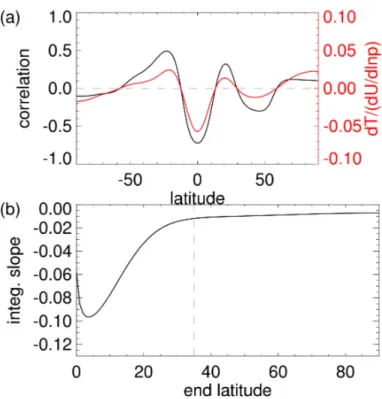
A1 Tropical average and QBO

Figure 7 shows the correlation and slope of the linear regression of deseasonalised zonal mean zonal wind shear at the equator with the zonal mean deseasonalised tem-perature for each latitude at 70 hPa. Figure 7b shows the (area weighted) slope of the linear regression integrated from the equator to the poles as function of the end latitude

25

(20)

ACPD

14, 13381–13412, 2014

Title Page

Tables Figures

◭ ◮

Back Close

Full Screen / Esc

Discussion

P

a

per

|

Discus

sion

P

a

per

|

Discussion

P

a

per

|

Discussion

P

a

per

|

belt (symmetric about the equator) where the effect of the QBO on temperature exactly cancels. For this study we have chosen the latitude belt 35◦S–35◦N as a compromise between a minimisation of QBO-related variance and focus on “tropical” temperatures. Results (not shown) using a latitude belt from 30S-30N instead of 35◦S–35◦N are very similar.

5

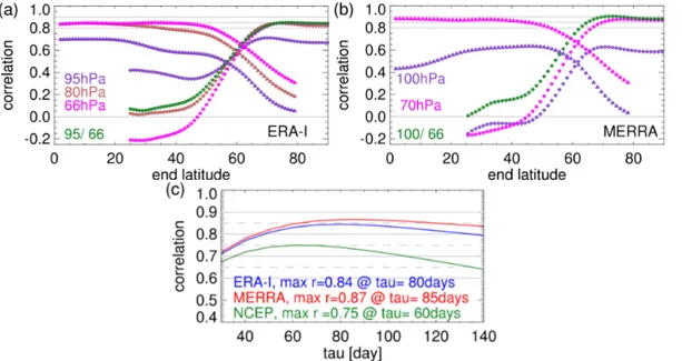
A2 Correlations between temperatures and proxy

Figure 8 shows the correlation coefficients between tropical average temperature and the proxy based on the eddy heat fluxes at the same pressure level for ERA-Interim and MERRA. The correlations are plotted as function of end latitude of the averaging domain of the eddy heat fluxes, with integration started at 20◦(diamonds), and

integra-10

tion started at 80◦. The figure shows that for 70 hPa, the proxy’s skill is primarily due to the heat fluxes between 40 and 80◦. For this study we have chosen to use the average between 25 and 75◦, but results with any proxy that includes the range between about 40 and 70◦ gives very similar results.

For 100 hPa, the correlations between proxy and temperature are, as expected,

15

weaker (the 100 hPa level in the tropics is in the middle of the TTL, and tropical processes play an important role; see discussion in Fueglistaler et al., 2009b). Also note the di_fferent behaviour between 100 hPa, and 80/66 hPa, with respect to eddy heat fluxes around 20–30◦. While 100 hPa temperatures are weakly positively corre-lated to the heat flux proxy at these latitudes, they are weakly negatively correcorre-lated at

20

80/66 hPa.

Acknowledgements. We thank RSS for providing the TLS temeprature data. MSU data are pro-duced by Remote Sensing Systems and sponsored by the NOAA Climate and Global Change Program. Data are available at www.remss.com.

We thank ECMWF for providing ERA-Interim reanalyses.

25

(21)

ACPD

14, 13381–13412, 2014

Title Page

Tables Figures

◭ ◮

Back Close

Full Screen / Esc

Discussion

P

a

per

|

Discus

sion

P

a

per

|

Discussion

P

a

per

|

Discussion

P

a

per

|

NCEP Reanalysis data provided by the NOAA/OAR/ESRL PSD, Boulder, Colorado, USA, from their Web site at http://www.esrl.noaa.gov/psd/.

SF and TJF acknowledge support from DOE grant SC0006841.

References

Baldwin, M. P., Gray, L. J., Dunkerton, T. J., Hamilton, K., Haynes, P. H., Randel, W. J., Holton,

5

J. R., Alexander, M. J., Hirota, I., Horinouchi, T., Jones, D. B. A., Kinnersley, J. S., Marquardt, C., Sato, K., and Takahashi, M.: The Quasi-Biennial Oscillation, Rev. Geophys., 39, 179–229, 2001. 13390

Bohlinger, P., Sinnhuber, B.-M., Ruhnke, R., and Kirner, O.: Radiative and dynamical contribu-tions to past and future Arctic stratospheric temperature trends, Atmos. Chem. Phys., 14,

10

1679–1688, doi:10.5194/acp-14-1679-2014, 2014. 13383, 13388

Dee, D. P., Uppala, S. M., Simmons, A. J., Berrisford, P., Poli, P., Kobayashi, S., Andrae, U., Balmaseda, M. A., Balsamo, G., Bauer, P., Bechtold, P., Beljaars, A. C. M., van de Berg, L., Bidlot, J., Borrmann, N., C.Delsol, Dragani, R., Fuentes, M., Geer, A. J., Haimberger, L., Healy, S. B., Hersbach, H., Holm, E. V., Isaksen, L., Kallberg, P., Köhler, M., Matricardi, M.,

15

McNally, A. P., Monge-Sanz, B. M., Morcrette, J.-J., Park, B.-K., Peubey, C., de Rosnay, P., Tavolato, C., Thepaut, J.-N., and Vitart, F.: The ERA-interim reanalysis: configuration and performance of the data assimilation system, Q. J. Roy. Meteor. Soc., 137, 553–597, 2011. 13387, 13393

Diallo, M., Legras, B., and Chédin, A.: Age of stratospheric air in the ERA-Interim, Atmos.

20

Chem. Phys., 12, 12133–12154, doi:10.5194/acp-12-12133-2012, 2012. 13385

Free, M.: The seasonal structure of temperature trends in the tropical lower stratosphere, J. Climate, 24, 859–866, 2011. 13383, 13392

Fu, Q., Solomon, S., and Lin, P.: On the seasonal dependence of tropical lower-stratospheric temperature trends, Atmos. Chem. Phys., 10, 2643–2653, doi:10.5194/acp-10-2643-2010,

25

2010. 13383, 13387

(22)

ACPD

14, 13381–13412, 2014

Title Page

Tables Figures

◭ ◮

Back Close

Full Screen / Esc

Discussion

P

a

per

|

Discus

sion

P

a

per

|

Discussion

P

a

per

|

Discussion

P

a

per

|

Fueglistaler, S., Legras, B., Beljaars, A., Morcrette, J.-J., Simmons, A., Tompkins, A. M., and Uppala, S.: The diabatic heat budget of the upper troposphere and lower/mid stratosphere in ECMWF reanalyses, Q. J. Roy. Meteor. Soc., 135, 21–37, 2009a. 13384

Fueglistaler, S., Dessler, A. E., Dunkerton, T. J., Folkins, I., Fu, Q., and Mote, P. W.: Tropical tropopause layer, Rev. Geophys., 47, RG1004, doi:10.1029/2008RG000267, 2009b. 13400

5

Fueglistaler, S., Haynes, P. H., and Forster, P. M.: The annual cycle in lower stratospheric tem-peratures revisited, Atmos. Chem. Phys., 11, 3701–3711, doi:10.5194/acp-11-3701-2011, 2011. 13386, 13391

Fueglistaler, S., Liu, Y.S, Flannaghan, T. J., Ploeger, F., and Haynes, P. H.: Departure from Clausius–Clapeyron scaling of water entering the stratosphere in response to changes in

10

tropical upwelling, J. Geophys. Res., 119, 1962–1972, doi:10.1002/2013JD020772, 2014. 13386

Hassler, B., Young, P. J., Portmann, R. W., Bodeker, G. E., Daniel, J. S., Rosenlof, K. H., and Solomon, S.: Comparison of three vertically resolved ozone data sets: climatology, trends and radiative forcings, Atmos. Chem. Phys., 13, 5533–5550, doi:10.5194/acp-13-5533-2013,

15

2013. 13383

Haynes, P. H., Marks, C. J., McIntyre, M. E., Shepherd, T. G., and Shine, K. P.: On the “down-ward control” of extratropical diabatic circulations by eddy-induced mean zonal forces, J. Atmos. Sci., 48, 651–678, 1991.

Hitchcock, T., Shepherd, T. G., and Yoden, S.: On the approximation of local and linear radiative

20

damping in the middle atmosphere, J. Atmos. Sci., 67, 2070–2085, 2010. 13386

Iwasaki, T., Hamada, H., and Myazaki, K.: Comparisons of Brewer–Dobson circulations diag-nosed from reanalyses, J. Meterol. Soc. Jpn., 87, 997–1006, doi:10.2151/jmsj.87.997, 2009. 13385

Kalnay, E., Kanamitsu, M., Kistler, R., Collins, W., Deaven, D., Gandin, L., Iredell, M., Saha,

25

S., White, G., Woollen, J., Zhu, Y., Leetmaa, A., Reynolds, R., Chelliah, M., Ebisuzaki, W., Higgins, W., Janowiak, J., Mo, K. C., Ropelewski, C., Wang, J., Jenne, R., and Joseph, D.: The NCEP/NCAR 40-year reanalysis project, B. Am. Meteorol. Soc., 77, 437–470, 1996. 13387

Lin, P., Fu, Q., Solomon, S., and Wallace, J. M.: Temperature trend patterns in Southern

Hemi-30

(23)

ACPD

14, 13381–13412, 2014

Title Page

Tables Figures

◭ ◮

Back Close

Full Screen / Esc

Discussion

P

a

per

|

Discus

sion

P

a

per

|

Discussion

P

a

per

|

Discussion

P

a

per

|

Mears, C. A. and Wentz, F. J.: Construction of the Remote Sensing Systems V3.2 Atmospheric Temperature Records From the MSU and AMSU Microwave Sounders, J. Atmos. Ocean. Tech., 26, 1040–1056, 2009. 13387

Newman, P. A. and Rosenfield, J. E.: Stratospheric thermal damping times, Geophys. Res. Lett., 24, 433–436, 1997.

5

Newman, P. A., Nash, E. R., and Rosenfield, J. E.: What controls the temperature of the Arctic stratosphere during the spring?, J. Geophys. Res., 106, 19999–20010, 2001. 13387, 13397 Pawson, S., Labitzke, K., and Leder, S.: Stepwise changes in stratospheric temperature,

Geo-phys. Res. Lett., 25, 2157–2160, 1998. 13391

Poli, P., Healy, S. B., and Dee, D. P.: Assimilation of Global Positioning System radio occultation

10

data in the ECMWF ERA-Interim reanalysis, Q. J. Roy. Meteor. Soc., 136, 1972–1990, 2010. 13393

Ramaswamy, V., Schwarzkopf, M. D., Randel, W. J., Santer, B.D, Soden, B. J., and Stenchikov, G. L.: Anthropogenic and natural influences in the evolution of lower strato-spheric cooling, Science, 311, 1138–1141, 2006. 13383

15

Randel, W. J., Garcia, R. R., and Wu, F.: Time-dependent upwelling in the tropical lower strato-sphere estimated from the zonal-mean momentum budget, J. Atmos. Sci., 59, 2141–2152, 2002. 13384, 13389, 13398

Randel, W. J., Wu, F., Oltmans, S. J., Rosenlof, K., and Nedoluha, G. E.: Interannual changes of stratospheric water vapor and correlations with tropical tropopause temperatures, J. Atmos.

20

Sci., 61, 2133–2148, 2004. 13397

Rienecker, M., Suarez, M. J., Gelaro, R., Todling, R., Bacmeister, J., Liu, E., Bosilovich, M. G., Schubert, S. D., Takacs, L., Kim, G.-K., Bloom, S., Chen, J., Collins, D., Conaty, A., Da Silva, A., Gu, W., Joiner, J., Koster, R. D., Lucchesi, R., Molod, A., Owens, T., Pawson, S., Pegion, P., Redder, C. R., Reichle, R., Robertson, F. R., Rudick, A. G., Sienkiewicz, M., and Woollen,

25

J.: MERRA: NASA’s modern-era retrospective analysis for research and applications, J. Cli-mate, 24, 3624–3648, doi:10.1175/JCLI-D-11-00015.1, 2011. 13387, 13393

Seviour, W. J., Butchart, N., and Hardiman, S. C.: The Brewer–Dobson circulation inferred from ERA-Interim, Q. J. Roy. Meteor. Soc., 38, 878–888,doi:10.1002/qj.966, 2012. 13385

Solomon, S., Young, P. J., and Hassler, B.: Uncertainties in the evolution of stratospheric ozone

30

(24)

ACPD

14, 13381–13412, 2014

Title Page

Tables Figures

◭ ◮

Back Close

Full Screen / Esc

Discussion

P

a

per

|

Discus

sion

P

a

per

|

Discussion

P

a

per

|

Discussion

P

a

per

|

SPARC CCMVal: SPARC Report on the Evaluation of Chemistry-Climate Models, edited by: Eyring, V., Shepherd, T. G., and Waugh, D. W., SPARC Report No. 5, WCRP-132, WMO/TD-No. 1526, 2010. 13384

Ueyama, R. and Wallace, J. M.: To what extent does high-latitude planetary wave breaking drive tropical upwelling in the Brewer–Dobson circulation?, J. Atmos. Sci., 67, 1232–1246,

5

doi:10.1175/2009JAS3216.1, 2010. 13383

Ueyama, R., Gerber, E. P., Wallace, J. M., and Frierson, D. M. W.: The role of high-latitude waves in the intraseasonal to seasonal variability of tropical upwelling in the Brewer–Dobson circulation, J. Atmos. Sci., 70, 1631–1648, 2013. 13388

Yulaeva, E., Holton, J. R., and Wallace, J. M.: On the cause of the annual cycle in tropical

10

(25)

ACPD

14, 13381–13412, 2014

Title Page

Tables Figures

◭ ◮

Back Close

Full Screen / Esc

Discussion

P

a

per

|

Discus

sion

P

a

per

|

Discussion

P

a

per

|

Discussion

P

a

per

|

Figure 1. (a)RSS Microwave Sounding Unit (MSU) lower stratospheric temperatures (MSU channel 4, or “TLS”), global (black), tropical (magenta) and combined extra-tropical (brown).

(b–d)Tropical (35◦S–35◦N) temperatures at 70 hPa and proxyT_p(eddy heat flux averaged over both hemispheres between 20 and 75◦, e-folded with∼80 day timescale; see text) for ERA-Interim (b), MERRA (c) and NCEP (d). Correlation coefficients refer to correlation between deseasonalised monthly means of tropical temperature and proxy over the period 1995–2011.

(26)

ACPD

14, 13381–13412, 2014

Title Page

Tables Figures

◭ ◮

Back Close

Full Screen / Esc

Discussion

P

a

per

|

Discus

sion

P

a

per

|

Discussion

P

a

per

|

Discussion

P

a

per

|

Figure 2. (a)Monthly trends in tropical (35◦S–35◦N) temperatures at 70 hPa from MERRA (red) and NCEP (green), and 67 hPa from ERA-Interim (red), for the period 1980–2011 (all years: lighter color; without 2 years following eruptions of El Chichon and Pinatubo: darker color).

(27)

ACPD

14, 13381–13412, 2014

Title Page

Tables Figures

◭ ◮

Back Close

Full Screen / Esc

Discussion

P

a

per

|

Discus

sion

P

a

per

|

Discussion

P

a

per

|

Discussion

P

a

per

|

(28)

ACPD

14, 13381–13412, 2014

Title Page

Tables Figures

◭ ◮

Back Close

Full Screen / Esc

Discussion

P

a

per

|

Discus

sion

P

a

per

|

Discussion

P

a

per

|

Discussion

P

a

per

|

(29)

ACPD

14, 13381–13412, 2014

Title Page

Tables Figures

◭ ◮

Back Close

Full Screen / Esc

Discussion

P

a

per

|

Discus

sion

P

a

per

|

Discussion

P

a

per

|

Discussion

P

a

per

|

Figure 5.Linear trends in the dynamically forced tropical 70 hPa temperature variations based on the 70 hPa eddy heat flux calculation for the period 1980–2011. The total forcing is the lin-ear sum of the contribution from each hemisphere, and the figure shows the trends for the total forcing (black) and for each hemisphere (brown: Northern Hemisphere; purple: Southern Hemi-sphere). Trends are shown for annual mean data (“all”), and for each month separately, labelled with the first letter of month. The proportionality between e-folded heat flux and temperature is calculated with a total least squares fit against observed temperature of the period 1995– 2011, using deseasonalised data. In addition to the statistical 1-sigma uncertainty in the trend, the thick lines shows the minimum-maximum range of the linear trend for the periods 1980– 2010, 1980–2011, 1981–2011. Note that in some months the trend uncertainty due to start/end point sensitivity is large compared to the statistical uncertainty over the period 1980–2011.(a)

(30)

ACPD

14, 13381–13412, 2014

Title Page

Tables Figures

◭ ◮

Back Close

Full Screen / Esc

Discussion

P

a

per

|

Discus

sion

P

a

per

|

Discussion

P

a

per

|

Discussion

P

a

per

|

(31)

ACPD

14, 13381–13412, 2014

Title Page

Tables Figures

◭ ◮

Back Close

Full Screen / Esc

Discussion

P

a

per

|

Discus

sion

P

a

per

|

Discussion

P

a

per

|

Discussion

P

a

per

|

(32)

ACPD

14, 13381–13412, 2014

Title Page

Tables Figures

◭ ◮

Back Close

Full Screen / Esc

Discussion

P

a

per

|

Discus

sion

P

a

per

|

Discussion

P

a

per

|

Discussion

P

a

per

|

Figure 8. Correlation between deseasonalised tropical average temperatures and tempera-ture proxy (see text) based on integrated eddy heat flux, convolved with e-folding timescale of 85 days, for pressure levels near 100, 80 (where available) and 70 hPa. Also shown (green) are the correlations between the e-folded eddy heat flux near 100 hPa with the temperatures near 70 hPa. Results are shown for(a) ERA-Interim, and (b) MERRA. (c) Correlation as function of relaxation time scaleτ for the eddy heat flux averaged over the latitude range 25–75◦